The HI Bias during the Epoch of Reionization
Wenxiao Xu, Yidong Xu, Bin Yue, Ilian T Iliev, Hy Trac, Liang Gao,, Xuelei Chen

TL;DR
This paper investigates how neutral hydrogen traces matter during the epoch of reionization using semi-numerical models, revealing scale-dependent bias evolution and a transition scale in the 21 cm line signal.
Contribution
It introduces a combined modeling approach to study HI bias evolution and scale dependence during reionization, highlighting a transition scale in the 21 cm bias.
Findings
Neutral hydrogen bias is negative on large scales during reionization.
The magnitude of the bias increases early and decreases late in reionization.
A transition scale exists where HI bias shifts from negative to positive.
Abstract
The neutral hydrogen (HI) and its 21 cm line are promising probes to the reionization process of the intergalactic medium (IGM). To use this probe effectively, it is imperative to have a good understanding on how the neutral hydrogen traces the underlying matter distribution. Here we study this problem using semi-numerical modeling by combining the HI in the IGM and the HI from halos during the epoch of reionization (EoR), and investigate the evolution and the scale-dependence of the neutral fraction bias as well as the 21 cm line bias. We find that the neutral fraction bias on large scales is negative during reionization, and its absolute value on large scales increases during the early stage of reionization and then decreases during the late stage. During the late stage of reionization, there is a transition scale at which the HI bias transits from negative on large scales to positive…
Click any figure to enlarge with its caption.
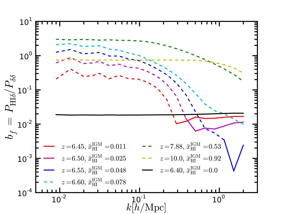 Figure 1
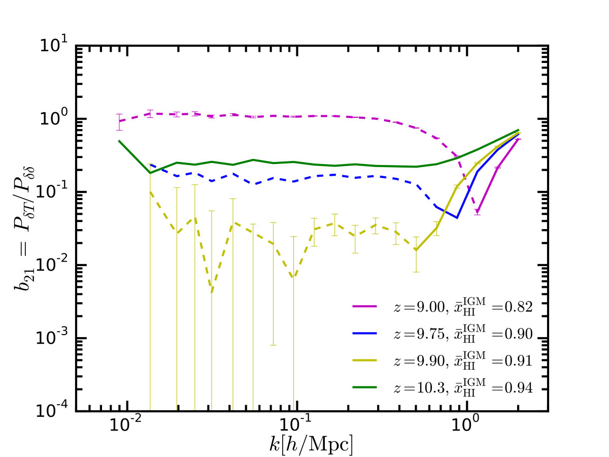 Figure 2
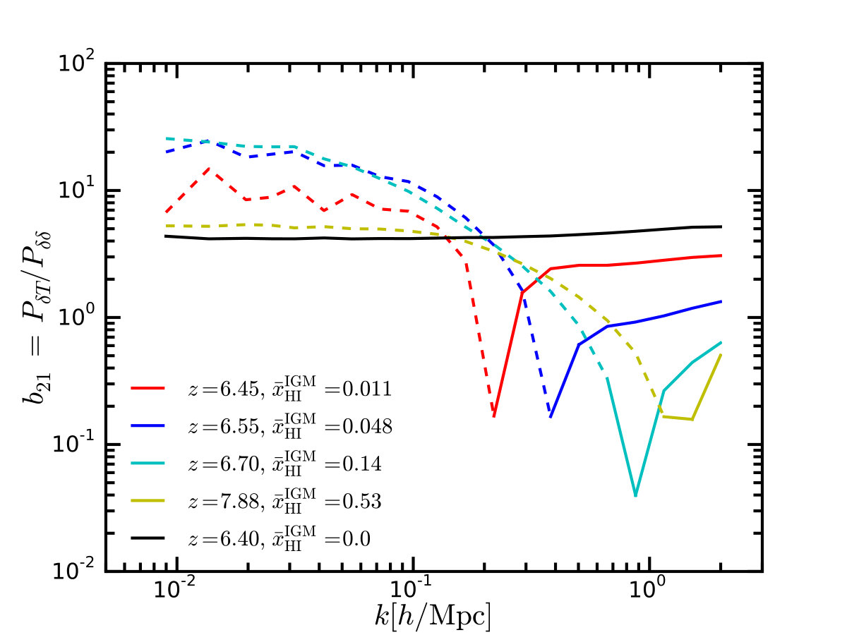 Figure 3
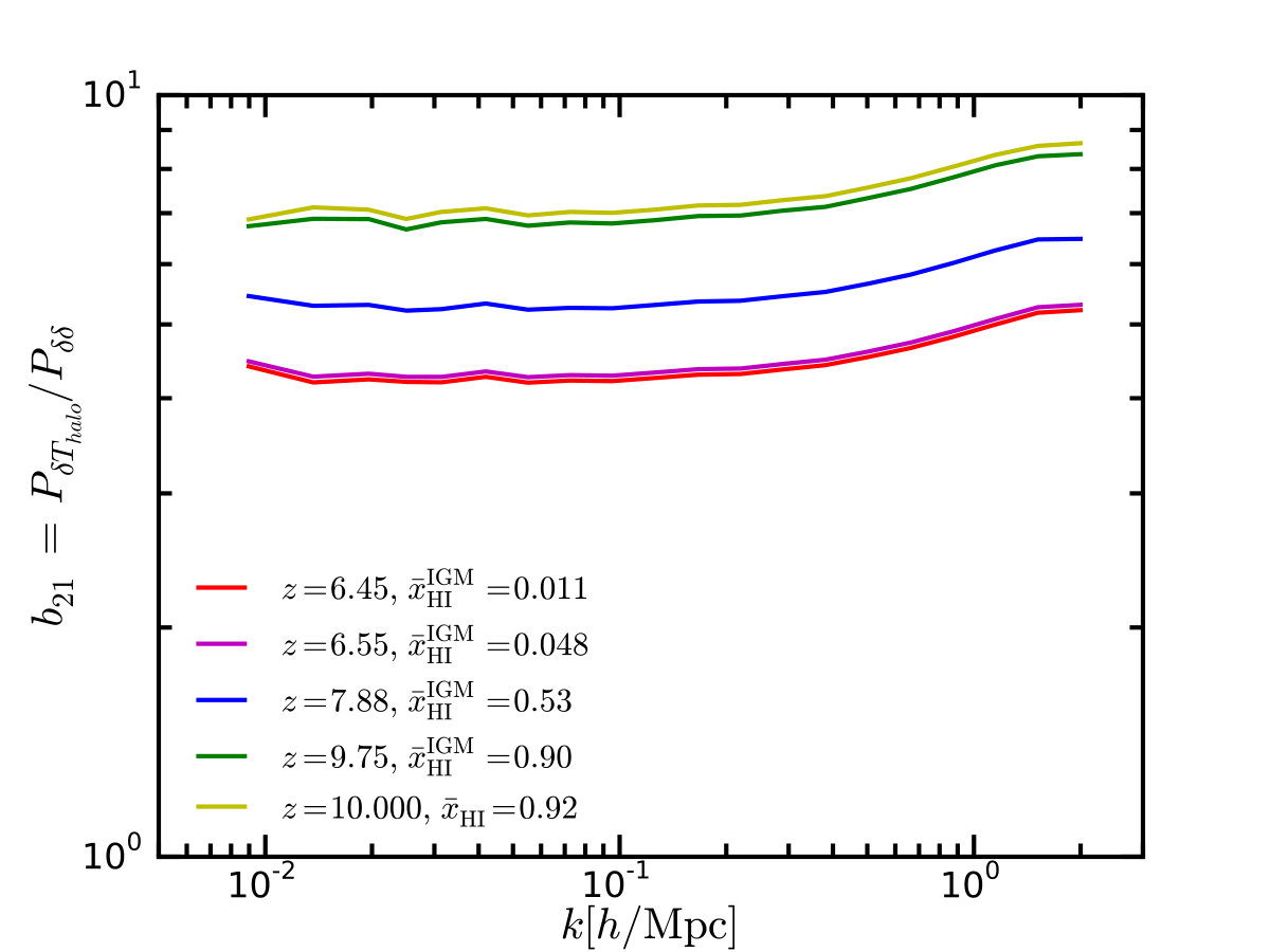 Figure 4
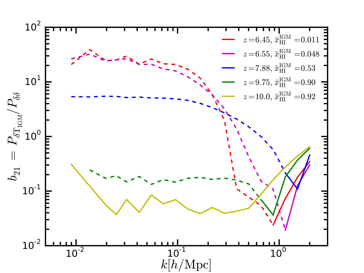 Figure 5
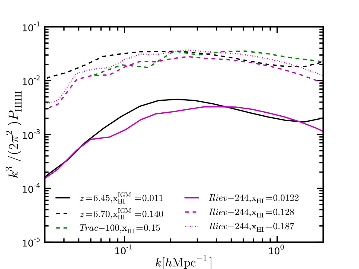 Figure 6
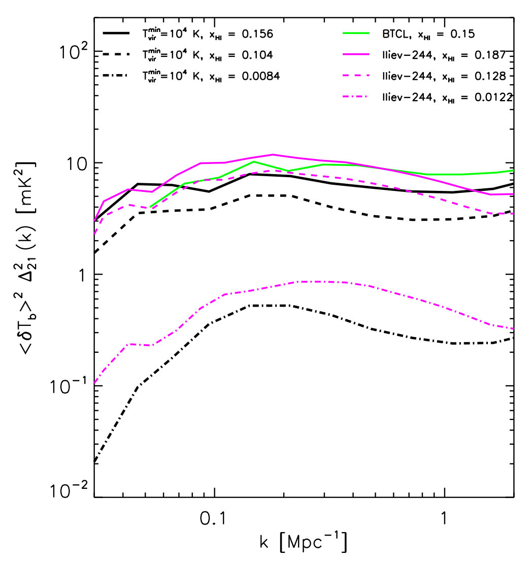 Figure 7
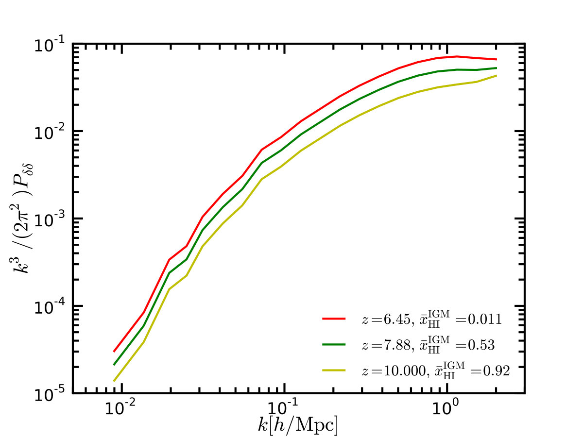 Figure 8
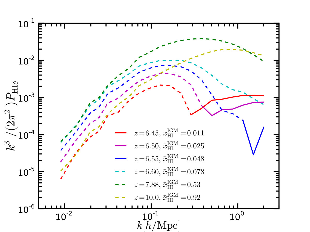 Figure 9
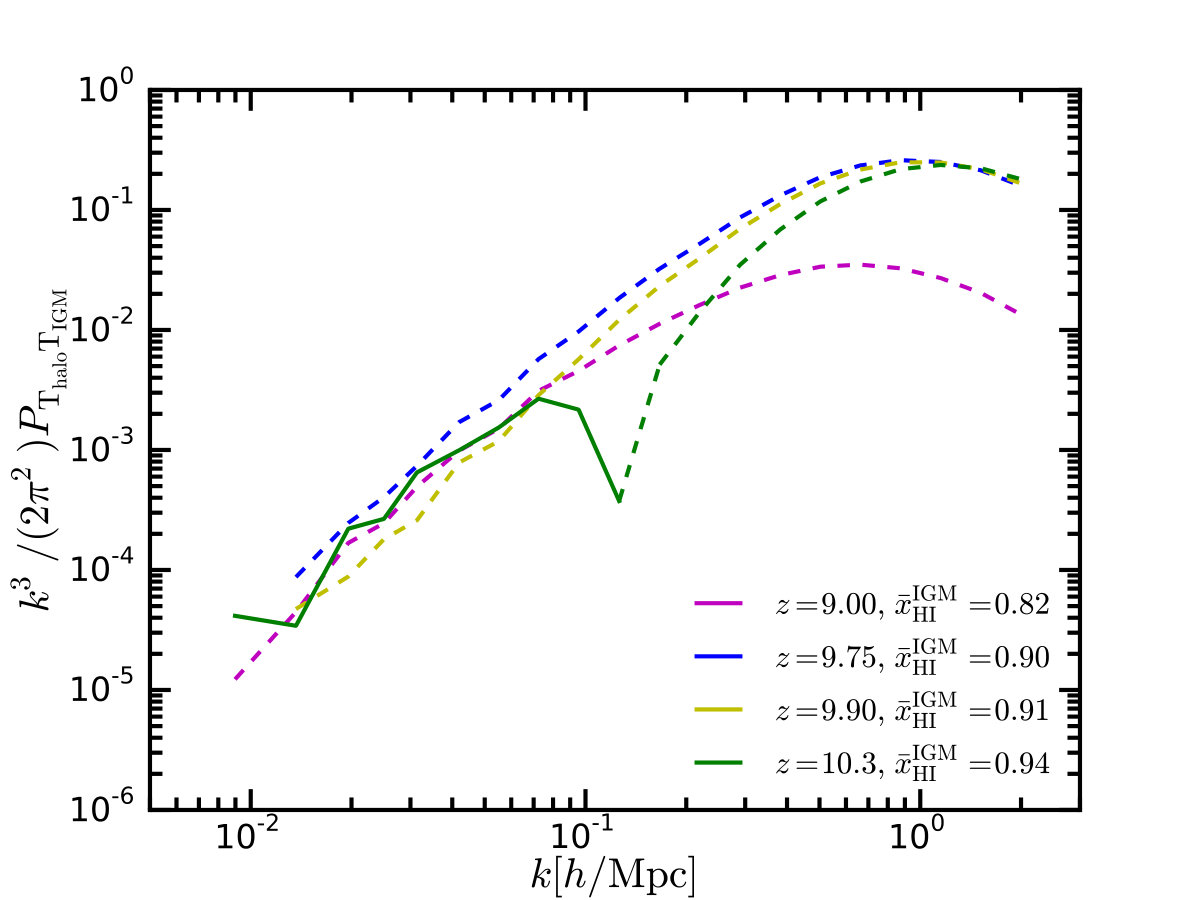 Figure 10
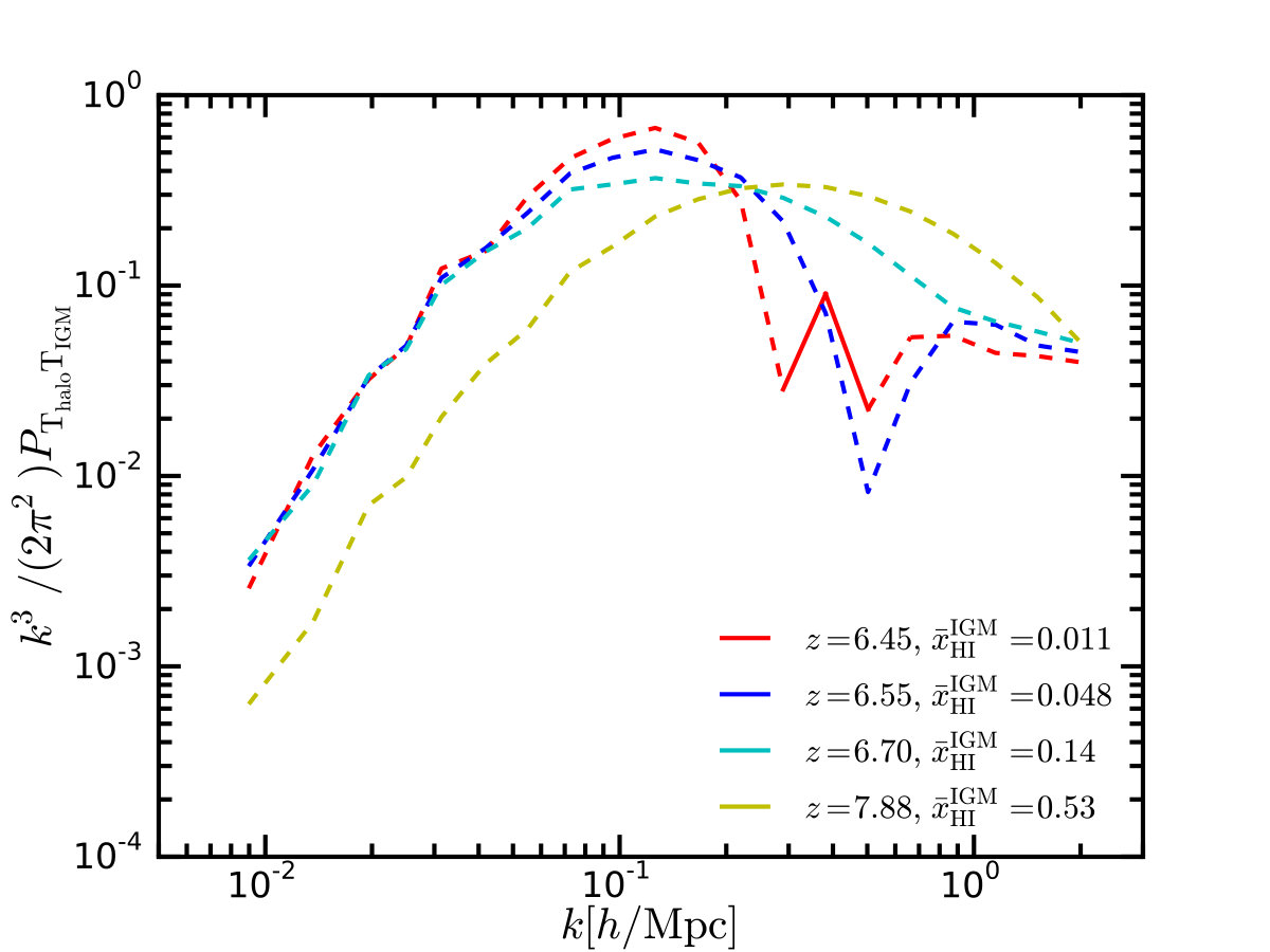 Figure 11
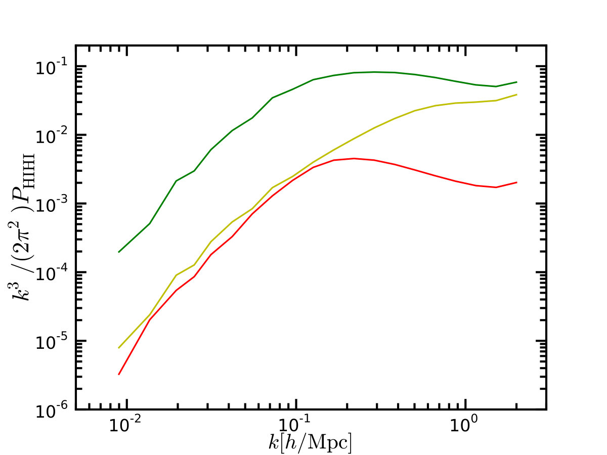 Figure 12
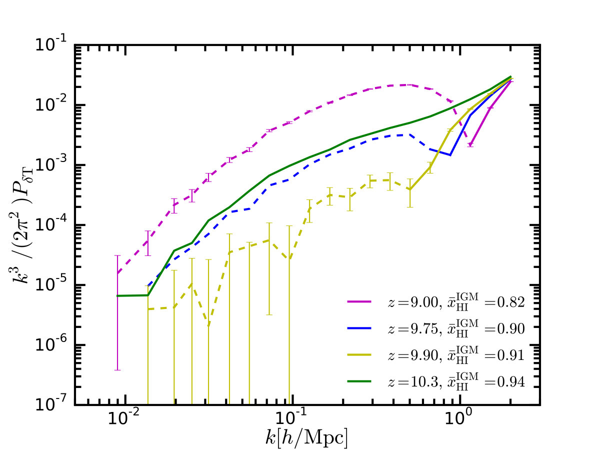 Figure 13
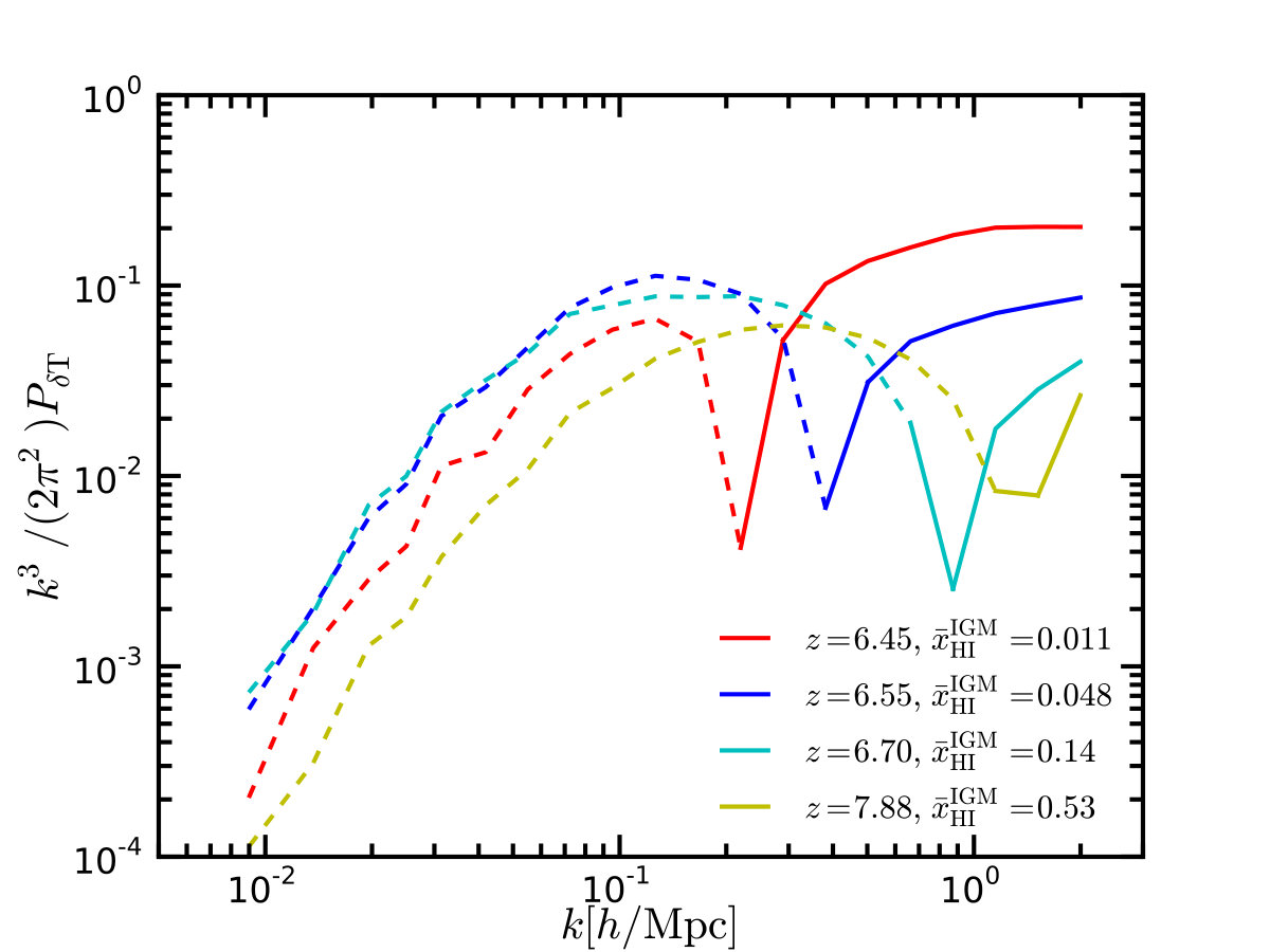 Figure 14
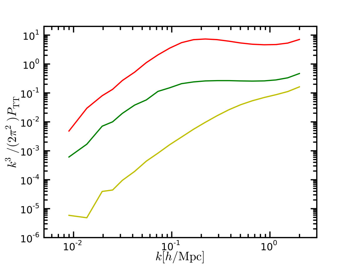 Figure 15
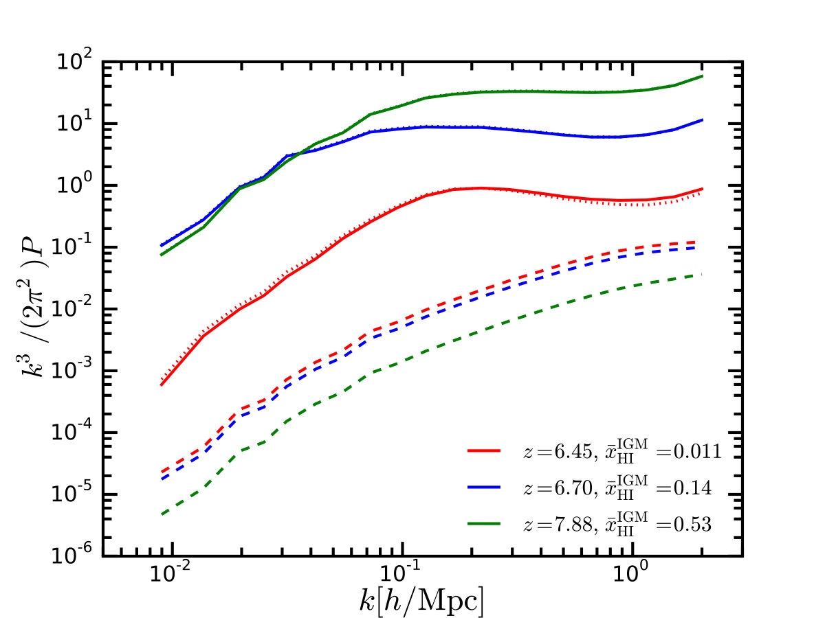 Figure 16
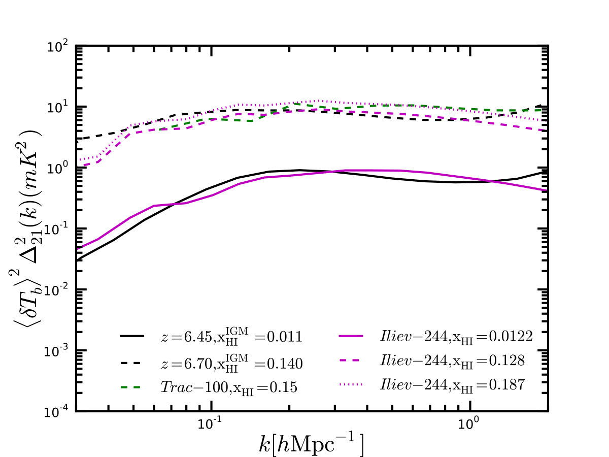 Figure 17
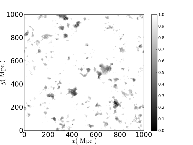 Figure 18
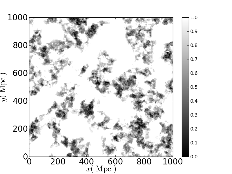 Figure 19
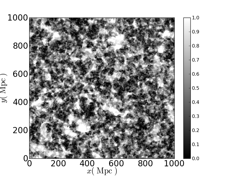 Figure 20
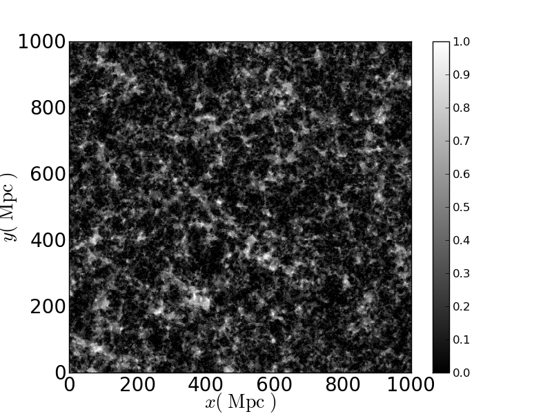 Figure 21
 Figure 22
Peer Reviews
No public reviews on file for this paper yet. If you reviewed it on a platform where reviews are public (OpenReview, ICLR, NeurIPS, ICML), you can paste yours below so the community can read it here.
Videos
No videos yet. Explain this paper in a talk, walkthrough, or lecture? Add one.
The HI Bias during the Epoch of Reionization
Wenxiao Xu,1,2 Yidong Xu1, Bin Yue1, Ilian T Iliev3, Hy Trac4, Liang Gao1, Xuelei Chen1,2
1Key Laboratory for Computational Astrophysics, National Astronomical Observatories, Chinese Academy of Sciences, Beijing, 100101, China
2 School of Astronomy and Space Science, University of Chinese Academy of Sciences, Beijing, 100049, China
3 Astronomy Centre, Department of Physics & Astronomy, University of Sussex, Falmer, Brighton, BN1 9QH, UK.
4 McWilliams Center for Cosmology, Department of Physics, Carnegie Mellon University Pittsburgh, PA 15213, USA E-mail: [email protected]
(Accepted XXX. Received YYY; in original form ZZZ)
Abstract
The neutral hydrogen (HI) and its 21 cm line are promising probes to the reionization process of the intergalactic medium (IGM). To use this probe effectively, it is imperative to have a good understanding on how the neutral hydrogen traces the underlying matter distribution. Here we study this problem using semi-numerical modeling by combining the HI in the IGM and the HI from halos during the epoch of reionization (EoR), and investigate the evolution and the scale-dependence of the neutral fraction bias as well as the 21 cm line bias. We find that the neutral fraction bias on large scales is negative during reionization, and its absolute value on large scales increases during the early stage of reionization and then decreases during the late stage. During the late stage of reionization, there is a transition scale at which the HI bias transits from negative on large scales to positive on small scales, and this scale increases as the reionization proceeds to the end.
keywords:
cosmology: theory–dark ages, reionization, first stars–large-scale structure of Universe
1 Introduction
The distribution of neutral hydrogen (HI) in the Universe contains a wealth of cosmological information. During the dark ages, the HI fluctuations follow the dark matter density perturbations; while during the epoch of reionization (EoR), the HI is anti-correlated with ionizing sources, and deviates from the total matter distribution. After reionization, however, most HI resides in halos, and once again can be used as a tracer of the large scale structure (LSS) of matter distribution over a wide range of redshifts and scales (Wang et al., 2019). Indeed, the 21 cm intensity mapping technique has been developed to more efficiently map the LSS of the Universe using HI as the tracer (Peterson et al., 2009). This technique is a promising probe of cosmological models (Bull et al. 2018; Xu et al. 2015, 2016; Obuljen et al. 2018b).
The 21 cm signals from the neutral component of the IGM are almost the unique feasible probe to major epochs of reionization by using current or upcoming radio telescopes (Alvarez et al., 2019; Furlanetto et al., 2019; Liu et al., 2019), such as the PAPER (Parsons et al., 2010), MWA (Bowman et al. 2013; Tingay et al. 2013), LOFAR (van Haarlem et al., 2013), HERA (DeBoer et al., 2017), SKA (Koopmans et al., 2015). However, reionization is a complicated process and at present our understanding is still mostly speculative. As other tracers of large scale structure, it is generally believed that on large scales the density of the neutral hydrogen should be proportional to the dark matter (DM) density with a nearly constant coefficient which we shall call “bias”. In order to interpret the upcoming 21 cm data from the EoR experiments, it is imperative to know the evolution and the scale-dependence of the bias of HI distribution, as well as the physical basis of its behavior.
There have been a number of investigations for the HI bias in the local and post-reionization Universe, using both observations and theory. For the low-redshift Universe, Martin et al. (2012) analyzed the bias of the HI-selected galaxies with in the ALFALFA survey, and found that on scales Mpc, the HI-selected galaxies are anti-biased with respect to DM, while on scales Mpc they are roughly unbiased. This is consistent with an earlier analysis for HIPASS samples (Basilakos et al., 2007). Marín et al. (2010) developed an analytic framework for the large-scale HI bias based on dark matter halo bias and a HI mass-halo mass relation. In Bagla et al. (2010) and Sarkar et al. (2016), the HI power spectrum and the related HI bias are derived by populating HI in halos identified in DM-only simulations. The HI bias in a wide redshift range () was investigated more explicitly by hydrodynamic simulations in Villaescusa-Navarro et al. (2018). To model the multi-phase hydrogen, they also post-processed the star-forming gas. They found that even at , the HI bias is already non-linear at Mpc*-1*.
During the EoR, however, most of the HI resides in the IGM. Various processes such as the formation of early galaxies and the non-linear bubble growth significantly complicate the bias of the HI distribution from the DM distribution. HI is not a very good tracer of the DM during this epoch, but it encodes rich information of reionization process and its driving sources. Hoffmann et al. (2018) have developed a quadratic model for the HI bias, which was found to work well during the early stage of reionization, and suggested that measurements of the three-point correlation functions in observations can constrain the astrophysical processes driving the reionization. McQuinn & D’Aloisio (2018) developed an effective perturbation theory, in which the 21 cm bias is expanded as the sum of terms whose coefficients reflect the bias of the ionizing sources, the global neutral fraction, the characteristic size of ionized regions and the patchiness of reionization. Still, the HI bias during the EoR is much less studied, especially for the transition stage: from the late EoR to the post-reionization. During this stage, the HI distribution is dominated by both the remaining neutral gas in halos, and the relic voids yet to be ionized, i.e., the “neutral islands” (Xu et al., 2014, 2017). The HI bias may show complicated and interesting behaviors. Knowing the HI bias would be convenient for deriving HI distribution statistics from the more simple dark matter distribution in theoretical works. In this work we shall study the HI bias during the EoR, especially in the transition era.
This paper is organized as follows. In Section 2, we present a model for the HI distribution during the EoR, including both the HI in the IGM from a set of semi-numerical simulations, and the HI in halos based on an empirical model. The results of the evolution and the scale dependence of the HI bias and 21cm bias are presented in Section 3. We summarize and discuss our results in Section 4. Throughout this paper, we assume the CDM model and adopt the following cosmological parameters : , , , , , and .
2 The HI Model
During and before the EoR, the neutral hydrogen exists in both IGM (as large diffuse patches of gas) and halos (as small dense clumps). We shall include both components in our model to properly account for the HI distribution.
2.1 The HI in the IGM
It is generally believed that reionization started first in high density regions where the first luminous objects formed first. In the “bubble model” of reionization (Furlanetto et al., 2004), the amount of star formation and the resulting ionizing photons are estimated using the excursion set model. Based on this idea, the so called “semi-numerical simulations" have been developed. For example, Mesinger et al. (2011) developed the 21cmFAST111https://github.com/andreimesinger/21cmFAST, to simulate the evolution of the 3D density, ionization and 21cm brightness temperature fields efficiently. The “bubble model” considers spherical regions of increasingly smaller scales and identifies ionized bubbles by comparing the cumulative number of ionizing photons produced within the region with the number consumed in reionization process. It has been demonstrated that the statistical predictions of the “bubble model” and the 21cmFAST agree fairly well with radiative-hydrodynamic simulations (Zahn et al., 2007; Mesinger et al., 2011; Zahn et al., 2011), at least when recombination, feedback, etc. are ignored. However, during most epochs of reionization, the topology of the ionization field is much more complicated than the isolated bubbles configuration. The bubbles start to connect with each other as early as when the global ionized fraction is just about 10%, and the Universe starts the percolation process when the ionized fraction gets 30% (see e.g. Furlanetto & Oh 2016; Chen et al. 2018). Inspired by the bubble model, the 21cmFAST determines the ionization state of each point by comparing the expected ionizing photon production in the surrounding region with the required number, but it allows non-spherical geometry for the ionized regions. In order to give a better description of the evolution of neutral regions after percolation, Xu et al. (2014) developed the so-called “island model”, assuming isolated neutral islands topology. The island model also takes into account an ionizing background that is inevitable during the late EoR (Furlanetto & Oh, 2005; Emberson et al., 2013; McQuinn et al., 2011). Based on the “island model”, a semi-numerical code named islandFAST was developed to mimic the islands evolution during the last stage of reionization (Xu et al., 2017). In the islandFAST, the effect of small-scale absorbers is taken into account empirically by adopting a fitting formula for the evolution of mean free path (MFP) of ionizing photons (Songaila & Cowie, 2010), based on the observed number density of Lyman limit systems up to redshift 6. Before the completion of reionization, the MFP is limited by both the under-dense islands and the over-dense absorbers. The evolution of the ionization field and the intensity of the ionizing background are derived self-consistently by an iterative procedure to ensure convergence in the total effective MFP of the ionizing photons.
Topological analysis shows that the islands become mostly isolated when the global neutral fraction reduces to in a model with parameters similar to the present case (Chen et al., 2018). In the island model the early stage of reionization is identical to that of the bubble model (21cmFAST) until , slightly before the isolation of individual islands, after which the island model criterion is applied for the later stages of reionization. For the following analysis, our simulation has a box size of 1 Gpc (comoving) on a side and a resolution of cells. An ionizing efficiency parameter of and a minimum virial temperature of K are adopted for host halos of ionizing sources. A few slices of the ionization field at several snapshots are shown in Fig. 1 .
2.2 The HI in halos
To model the HI in halos, for each cell in the simulation box with a size of and a mass of at redshift , the number density of halos with mass virialized at in this cell, , can be estimated by using the conditional mass function (Cooray & Sheth, 2002):
[TABLE]
where
[TABLE]
Here is the mean matter density of the present Universe and is the critical density; is critical density required for spherical collapse at , denotes the initial density for a region to have density at , is the variance of the density fluctuations on scale , and we adopt the form of given in Sheth & Tormen (1999). The relation between the HI mass and its host halo mass has been widely studied (Gong et al., 2011; Popping et al., 2015; Guo et al., 2017; Padmanabhan & Refregier, 2017; Villaescusa-Navarro et al., 2018; Obuljen et al., 2018a). Here we adopt the results from a large state-of-the-art hydrodynamic simulation, TNG100 (Villaescusa-Navarro et al., 2018), for which the result can be fitted by
[TABLE]
The parameters are given for a number of redshifts. At , , , and (Villaescusa-Navarro et al., 2018). We adopt these parameter values throughout the reionization history, as that is the highest redshift where the values are given, and also the relations vary little near . Another possibility is to fit the redshift dependence at , then extrapolate to higher redshifts. We have checked that such extrapolation gives similar results, but given the uncertainty, it is not clear if a better accuracy can be achieved. The HI content of a halo may also depends on its assembly history and when the local patch was ionized. Obviously, there are always some theoretical uncertainties in the model of HI gas in halos during the EoR, both intrinsic and environmental, which one must bear in mind.
The neutral fraction of a given cell with mass and volume contributed by HI in halos can be written as
[TABLE]
where donates the hydrogen mass fraction in the gas, . The HI in halos are combined with the HI in the IGM, predicted by semi-numerical simulations such as the 21cmFAST or islandFAST, to generate the full HI field at various redshifts throughout the reionization. In the following, we denote the neutral fraction in the IGM as , the neutral fraction contributed from the HI in halos as , and denote the total neutral fraction as .
3 The HI Bias throughout the EoR
The formation of galaxies and the evolution of the IGM are physical consequences of the primordial density perturbations. On large scales, the observables such as the galaxy number density, the neutral hydrogen fraction of the IGM or the 21cm brightness temperature should be related to the locally averaged matter density. Here we approximate such relation with a linear model, though more generally the relation may be non-linear and stochastic (Dekel & Lahav, 1999).
The reionization process is believed to be “inside-out” (e.g. Iliev et al. 2006; Trac & Cen 2007) on large scales: galaxies formed firstly in over-dense regions, and ionized their surrounding gas, then the reionization proceeds from the over-dense regions to the mean and under-dense regions. In this scenario, it is expected that the neutral hydrogen is anti-correlated with the underlying dark matter density distribution on large scales. However, this relation could be inverted on small scales, where the neutral hydrogen in halos is correlated with the density, and also the ionization front moves faster into the void regions. The non-linear structure growth, galaxy formation, ionizations and feedbacks would significantly complicate the neutral hydrogen-density relation and hence the HI bias. The time- and scale-dependence of the HI bias encodes rich information about the reionization process.
The neutral hydrogen is observationally traced by the 21 cm signal, the upcoming low-frequency interferometers will directly measure the fluctuations in the 21 cm brightness temperature. Ignoring the peculiar velocities, the 21 cm brightness temperature is related to the neutral fraction , the density contrast , and the spin temperature via (e.g. Pritchard & Loeb 2012)
[TABLE]
where is the background photon temperature, and in the absence of very strong radio sources it would be given by the cosmic microwave background temperature at that redshift. Although when the first stars formed might be lower than (Chen & Miralda-Escudé, 2004, 2008), after a moderate fraction of gas had been ionized, the rest of the neutral HI would be heated to . For simplicity here we shall assume this relation holds through the whole EoR process. To calculate the contributions to the 21cm signal from halos and the IGM separately, one can replace the with or with . Strictly speaking, Eq. (5) is only valid in the optically-thin limit, which may not be true for HI gas in halos. However, it has been shown that for the average of from many halos, it is still a good enough approximation (Yue et al., 2009).
The neutral fraction bias can be computed by comparing the power spectra of the neutral fraction field and dark matter density field, either from the auto-power spectrum
[TABLE]
or from the cross-power spectrum
[TABLE]
where
[TABLE]
are the matter power spectrum, neural fraction power spectrum, and cross-power spectrum between the two, respectively, and are the Fourier transform of and dark matter density contrast respectively, and denotes the the expectation value with the Dirac delta function removed. The bias defined in this way can be negative, this is similar to the bias of voids (Sheth & van de Weygaert, 2004; Chan et al., 2014). We shall use Eq. (7) which is less affected by the stochasticity and the shot noise term (Villaescusa-Navarro et al., 2018), and also there is no ambiguity in the sign of the bias. Similarly, we also compute the 21cm bias using
[TABLE]
where is the Fourier transform of and . Throughout this paper for the 21cm power spectrum or 21cm-dark matter cross-power spectrum we adopt the dimensionless definition.
3.1 The power spectra
In the present work, the reionization process is simulated by the 21cmFAST for early stage and by the islandFAST after percolation. The 21 cm power spectrum predicted by the 21cmFAST was previously presented and discussed in Mesinger et al. (2011). While the 21 cm power spectrum during the late stages of reionization was also discussed in Giri et al. (2019), here we compare the islandFAST predictions with the radiative-hydrodynamic simulations by Battaglia et al. (2013) (Trac-100 simulation) and by Dixon et al. (2016) (Iliev-244 simulation) at some similar neutral fractions. The neutral fraction power spectra and the 21cm power spectra, in the limit of , are plotted in the upper and lower panels of Fig. 2, respectively. The black solid and dashed lines correspond to neutral fractions of and 0.14, respectively from islandFAST. Here the box sizes are for the Trac-100 simulation (green line), and for the Iliev-244 simulation (magenta lines), respectively. Generally, these neutral fraction and the 21 cm power spectra have similar shape on large scales. Considering the differences between the two numerical simulations and output neutral fractions, these differences are probably not very significant, though the inclusion of evolutional small scale ionizing photons absorbers in the islandFAST semi-numerical code may also contributed to the difference.
The dark matter density power spectra (e.g.Santos et al. 2010; Iliev et al. 2014), as well as the 21 cm power spectra (e.g. Mesinger & Furlanetto 2007; Kim et al. 2016) during the EoR have been studied in a number of previous simulations. In this subsection, we calculate the power spectra from our simulation, in the same convention as the ones in the bias formula (Eq.(7) – (9) ). In addition to the matter density and 21 cm power spectra, here we also calculate the neutral fraction power spectra, as well as the cross-power between them, in order to gain a better understanding of the bias behavior to be presented in the next subsections.
In Fig. 3 we plot the dark matter power spectra (top panel), the power spectra for the neutral fraction field (middle panel) and 21cm brightness temperature field (bottom panel) in our model during the EoR. In the top panel, the three curves from bottom to top are for the early, intermediate and late stages of reionization, respectively, and in the middle and bottom panels the corresponding curves are plotted with the same colors as the top panel.
The power spectrum of the dark matter density fluctuations steadily increase as the redshift decreases, while keeping the shape almost unchanged on the scales discussed here. By contrast, neither the redshift evolution nor the scale dependence of the neutral fraction power spectrum is monotonic. The neutral fraction power spectrum first increases during the early stage of reionization, and then decreases during the late stage of reionization. The 21cm power spectrum, however, keeps increasing with decreasing redshift until . Note here we are referring to the dimensionless power, and part of the increase of the power comes from the decreasing mean 21cm brightness temperature as more regions are ionized. In the late stage of reionization, there is a bump around /Mpc on both of them. This scale is close to the typical ionized bubble size, and the HI fluctuations at smaller scales are somewhat suppressed by reionization process.
The cross-power spectrum between the neutral fraction field and the dark matter density field is shown in Fig.4. We use dashed lines to mark the negative power, while solid lines refer to positive power. As seen in this figure, during most of the EoR stages, the neutral fraction field is anti-correlated with the dark matter density field, resulting in negative cross-power spectrum. As the reionization proceeds, the amplitude of the large scale cross-power spectrum increases during the early stage of reionization, reaches its maximum roughly at the mid point of reionization, then decreases during the late stage. When the IGM global neutral fraction drops below , on the small scales a positive cross-correlation appears. At this stage, most of the IGM has been ionized, while the neutral hydrogen in halos starts to dominate the cross power spectrum, producing the positive correlation seen in the small scale power spectrum. As the remaining neutral islands in the IGM shrink and decrease in number, the halo HI come to dominate the fluctuations on larger and larger scales, as a result this positive-to-negative transition point on the cross-power spectrum moves to larger scales.
The cross-power spectrum between the 21cm brightness temperature and the dark matter density are plotted in Fig. 5. We use the two panels to show the early and late stages of reionization respectively. We find that at the very beginning of reionization, the 21cm-dark matter cross-power spectrum is positive on all scales, implying that the neutral hydrogen density fluctuations still follow the dark matter density fluctuations, although some rare density peaks have been ionized. As more and more IGM around density peaks becomes ionized, the 21cm-dark matter cross-power spectrum decreases, and transits to negative starting from the largest scales. Then the large scale 21cm-dark matter cross-power becomes more and more negative. The amplitude reaches its maximum at around , and decreases again. Different from the -dark matter cross-power, the 21cm-dark matter cross-power spectrum is always positive at small scales, indicating that when weighted with the local density, the small scale 21 cm signal is always dominated by the HI in halos. At the very late stage of reionization, the positive-to-negative transition scale increases rapidly.
In this plot the 21cm-dark matter cross-power spectrum at shows some oscillations, which are likely statistical fluctuations. To check this interpretation, we estimate the errors on cross-power spectra by using the jackknife resampling method. In Fig. 5 we plot the errors for the z=9.90 and z=9.00 curves. To avoid clutter, errors of other curves are not shown there. We see that indeed at z=9.90 the error bars are larger than the oscillation feature on the power spectrum curve, so it is likely that these are just statistical fluctuations. We also check that at z=9.00 the errors are comparable with the z=9.90. However, at z=9.00 the cross-power spectrum is much larger than z=9.90. In logarithmic axes apparently its errors are less obvious than z=9.90.
We then turn to the individual contribution from the IGM and halos to the 21cm power spectrum, see Fig. 6. The power spectrum of the HI in the IGM evolves markedly, in contrast to the power spectrum of the HI in halos. During the era studied here, the full 21cm power spectrum is dominated by the IGM contribution in our model, though we note here that we assumed a constant relation, if it evolves this conclusion would be revised, though the evolution in this relation is perhaps still much less significant than that in the IGM.
Fig. 7 shows the cross-power between the 21cm brightness contributed from the IGM and that from halos during the early (top panel) and late EoR (bottom panel). Generally these two components are anti-correlated during the EoR, except at the very early stage () when the ionized bubbles only occupy a tiny fraction, there are still positive cross-correlation on large scales ( Mpc*-1*).
3.2 The neutral fraction bias
In Fig. 8, we show the scale dependence of the neutral fraction bias at various stages of reionization. As the dark matter power spectrum evolves almost self-similarly throughout the EoR, the evolution of neutral fraction bias basically follows the trend in the cross-power spectrum . As discussed above, during most of the EoR the HI in the IGM makes a negative contribution to the bias, while HI in halos makes a positive contribution. Before the end of reionization, the total bias is negative on large scales. When , it is negative on all scales, which is expected in the “inside-out” model of the reionization process. In over-dense regions, the HI fraction is lower than in the under-dense regions, resulting in an anti-correlated relation. Note however that the absolute amount of the remaining HI content in the over-dense regions is not necessarily smaller than in the under-dense regions. Regarding the -dependence of the , there is a typical scale, below which drops gradually, while almost independent of above this typical scale. This typical scale increases as reionization process goes on, reflecting the bubble growth process during the EoR.
We do expect the bias to be scale-independent on large scales: if we smooth the density field by a filter much larger than ionized bubbles, the density field becomes rather smooth, i.e. , where is the mean density contrast within the smoothing radius. In such case for a region with mass and mean density contrast the mean neutral fraction , or , where
[TABLE]
is the collapse fraction and is the mean recombination number per H atom. For we have , and as a result at large scale the HI bias is broadly scale-independent.
When , HI in the IGM is dominant and the halo HI has a negligible contribution to the total HI. During this stage, on small scales the amplitude of the negative bias decreases rapidly as reionization proceeds. However, on large scales, at the beginning the amplitude is smaller, because is rather uniform and close to almost everywhere. As decreases , the amplitude first increases to a peak amplitude when the Universe is about half-ionized, then decreases as well. When decreases to below , HI in halos starts to dominate the small scale fluctuations and the positive starts to appear at the small scales. A transition scale, at which the transits from negative at larger scales to positive at smaller scales, increases with the neutral islands being ionized and the increasing contribution by HI in halos.
We also plot the after the completion of reionization in Fig. 8. As expected, after the HI in the IGM gets all ionized, the remaining HI in halos positively correlate with the underlying matter density, resulting in the positive bias at all scales after reionization. Note that after reionization, the is basically a weighted halo bias on scales larger than the cell size of our simulation. As we have neglected the rare halos with masses larger than the cell mass and smoothed the HI density within cells, we have equivalently neglected the one-halo term contribution to the power spectrum, and retained only the two-halo term on large scales (Cooray & Sheth, 2002), which results in an under-estimate of the bias on small scales. Also, we note that the halo model, as well as our method of populating simulation cells using the conditional mass function, would under-estimate the halo bias on scales as compared to that from N-body simulations. Both of these effects give rise to the nearly scale-independent bias on the relevant scales. Interestingly, the neutral fraction bias transits from fully negative to fully positive in a very short time scale, which is a clear indication of the completion of reionization.
3.3 The 21 cm bias
The evolution of the 21cm bias during the early and late stages of reionization is shown in Fig. 9. The error bars for the and curves are derived by similar method as Fig. 5. Unlike the neutral fraction bias, the 21cm bias shows more complicated behavior, especially in the early stage of EoR. The 21cm bias is always positive on small scales, showing the dominance of the HI in halos. However the neutral fraction bias is totally negative in the small scales at early EoR, because the 21cm signal is weighted by local density, and the halo contribution is more apparent.
On large scales, the 21cm bias is positive at the beginning of reionization, then decreases to below zero and becomes more and more negative during the early EoR, and then increases again and becomes less and less negative during the late EoR. During most of the EoR, there is a transition point at which the 21cm bias transits from negative at large scales to positive at small scales, and this transition scale only shows an obvious increase in the late EoR. Perhaps due to this shift of transition scale, the bias is scale-dependent up to fairly large scales during the late EoR. We also show the after the completion of reionization, which is a positive horizontal line in the figure, similar to the .
We plot the 21cm bias for HI in halos as well as in the IGM in Fig. 10. Similar to the cross-power spectra discussed in Sec. 3.1, on large scales the 21cm bias is dominated by the IGM while on small scales it is dominated by halos. A critical scale, below which halos contribute more to the 21cm bias than the IGM, increases with the decreasing redshift. Here we note that even considering only the IGM contribution, the 21cm bias is still positive on the smallest scales. This is due to the density fluctuations in the neutral regions: there are some relatively over-dense regions even in the under regions but not dense enough to collapse and produce ionizing photons.
We tested the resolution convergence of our simulation by using a simulation with higher resolution ( cells) and smaller box size (286 Mpc per side) while keeping other parameters the same as our fiducial simulation. The density and ionization fields are smoothed to the same resolution as our fiducial simulation, then the halo HI content in each cell is assigned using the same model as described in section 2.2. The neutral fraction bias of this higher resolution simulation and our fiducial simulation at the same redshift are shown in Fig. 11. We see that they agree with each other. More importantly, the transition scales at which the changes the sign agrees with each other very well, indicating the robustness of our conclusions.
4 Conclusions and discussions
In this paper, we investigated the HI distribution thoughout the EoR, including the HI in the IGM from semi-numerical simulations, and the HI in halos from an empirical relation between HI mass and its host halo mass. We focused on the bias of the HI distribution with respect to the underlying matter density distribution, in terms of the neutral fraction bias and the 21cm brightness temperature bias.
We found that during the reionization stage when , the neutral fraction bias is always negative at all scales. However the amplitude first increases, up to the maximum when , then decreases. When , positive bias appears at the smallest scales. Since then the negative-to-positive transition scale keeps increasing as the reionization approaches to the end in a short time scale. It is a good indicator of the completion of the reionization process.
The 21cm bias, however, is more complicated than the neutral fraction bias. Compared with neutral fraction, the 21cm brightness temperature is weighted by local gas density, therefore more correlated with the dark matter. At the smallest scales, the 21cm bias is always positive throughout the EoR, due to the contribution from HI in small neutral islands and in halos. At large scales, the 21cm bias is positive at the early EoR stage, however its amplitude decreases with decreasing IGM neutral fraction. At , the large scale 21cm bias transits from positive to negative. Since then the bias amplitude rises again, reaching its maximum absolute value when the IGM is roughly at . From then on, the amplitude of the large scale 21cm bias drops again. However, at the same time the small scale 21cm bias always keeps increasing, because the contribution from HI in halos becomes more and more important. As a result, the transition point at which the 21cm bias transits from positive to negative, keeps increasing. Finally the reionization completed and all 21cm bias becomes positive again.
In summary, a transition of 21cm bias from positive to negative at large scales marks the starting of reionization, while 21cm bias reverts negative to positive on large scales with the completion of reionization.
The 21cm fluctuation could be measured with the current or upcoming generation experiments such as LOFAR, MWA, HERA or SKA-low. The dark matter distribution and its cross-correlation with 21cm studied here can not be measured directly, but by cross-correlating the 21cm brightness field and some tracers of dark matter density, the 21cm bias can still be derived. The 21cm-dark matter cross correlation and bias is however more general than specific tracers. A number of high redshift observations can be used to trace the large scale dark matter density, for example the Lyman Break Galaxies (LBGs) and Ly emitters (LAEs) derived from broadband or narrow band photometric observations (Dayal & Ferrara, 2012; Garel et al., 2015; Bouwens et al., 2015). Of course, there will also some bias of the tracer sample with respect to the dark matter. Indeed, Sobacchi et al. (2016) and Kubota et al. (2018) have investigated the detectability of 21cm-LAE cross-correlation by combining the Subaru Hyper-Suprime Cam (HSC) Ultra-Deep field survey (Aihara et al., 2018a, b) and the upcoming 21cm survey with LOFAR, MWA, or SKA-low. Measurement of the cross-correlation with the SKA-low is found very promising, and we expect the 21cm bias and its evolutionary features could be determined via such measurement in the SKA era.
Acknowledgements
We thank Renyue Cen, Kwan Chuen Chan and Francisco Villaescusa-Navarro for helpful discussions. This work is supported by the the National Natural Science Foundation of China (NSFC) key project grant 11633004, the NSFC-ISF joint research program No. 11761141012, the CAS Frontier Science Key Project QYZDJ-SSW-SLH017, Chinese Academy of Sciences (CAS) Strategic Priority Research Program XDA15020200, and the MoST 2016YFE0100300. BY also acknowledges the support of the CAS Pioneer Hundred Talents (Young Talents) program, the NSFC grant 11653003, the NSFC-CAS joint fund for space scientific satellites No. U1738125. ITI was supported by the Science and Technology Facilities Council [grant numbers ST/I000976/1, ST/F002858/1 and ST/P000525/1];and The Southeast Physics Network (SEPNet). We acknowledge that the results in this paper have been achieved using the PRACE Research Infrastructure resources Curie based at the Trs Grand Centre de Calcul (TGCC) operated by CEA, France and Marenostrum based in the Barcelona Supercomputing Center, Spain.The authors gratefully acknowledge the Gauss Centre for Supercomputing e.V.(www.gauss-centre.eu) for funding this project by providing computing time through the John von Neumann Institute for Computing (NIC) on the GCS Supercomputers JURECA and JUWELS at Juelich Supercomputing Centre (JSC)
The reference list from the paper itself. Each links out to its DOI / PubMed record.
- 1Aihara et al. (2018 a) Aihara H., et al., 2018 a, PASJ , 70, S 4 · doi ↗
- 2Aihara et al. (2018 b) Aihara H., et al., 2018 b, PASJ , 70, S 8 · doi ↗
- 3Alvarez et al. (2019) Alvarez M. A., et al., 2019, ar Xiv e-prints ( ar Xiv:1903.04580 )
- 4Bagla et al. (2010) Bagla J. S., Khandai N., Datta K. K., 2010, MNRAS , 407, 567 · doi ↗
- 5Basilakos et al. (2007) Basilakos S., Plionis M., Kovač K., Voglis N., 2007, MNRAS , 378, 301 · doi ↗
- 6Battaglia et al. (2013) Battaglia N., Trac H., Cen R., Loeb A., 2013, Ap J , 776, 81 · doi ↗
- 7Bouwens et al. (2015) Bouwens R. J., et al., 2015, Ap J , 803, 34 · doi ↗
- 8Bowman et al. (2013) Bowman J. D., et al., 2013, Publications of the Astronomical Society of Australia , 30, e 031 · doi ↗