Radiality Constraints for Resilient Reconfiguration of Distribution Systems: Formulation and Application to Microgrid Formation
Shunbo Lei, Chen Chen, Yue Song, and Yunhe Hou

TL;DR
This paper introduces a novel radiality constraint formulation for distribution system reconfiguration, enhancing flexibility and optimality, especially in microgrid formation for resilience, validated through theoretical and case study analyses.
Contribution
It proposes a new radiality constraints method that fully enables topological flexibilities in distribution systems, improving feasibility and optimality in reconfiguration problems.
Findings
Enhanced microgrid formation model with flexible merge/separation
The new constraints improve solution feasibility and optimality
Case studies demonstrate superiority over existing models
Abstract
Network reconfiguration is an effective strategy for different purposes of distribution systems (DSs), e.g., resilience enhancement. In particular, DS automation, distributed generation integration and microgrid (MG) technology development, etc., are empowering much more flexible reconfiguration and operation of the system, e.g., DSs or MGs with flexible boundaries. However, the formulation of DS reconfiguration-related optimization problems to include those new flexibilities is non-trivial, especially for the issue of topology, which has to be radial. That is, existing methods of formulating radiality constraints can cause underutilization of DS flexibilities. Thus, this work proposes a new method for radiality constraints formulation fully enabling the topological and some other related flexibilities of DSs, so that the reconfiguration-related optimization problems can have extended…
Click any figure to enlarge with its caption.
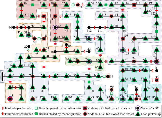 Figure 1
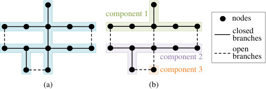 Figure 2
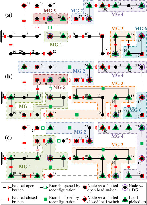 Figure 3
 Figure 4
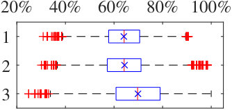 Figure 5
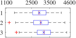 Figure 6
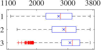 Figure 7
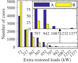 Figure 8
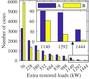 Figure 9
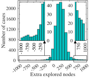 Figure 10
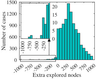 Figure 11
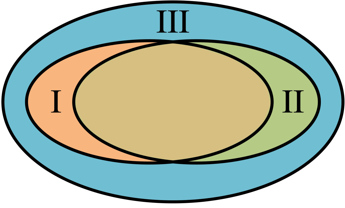 Figure 12
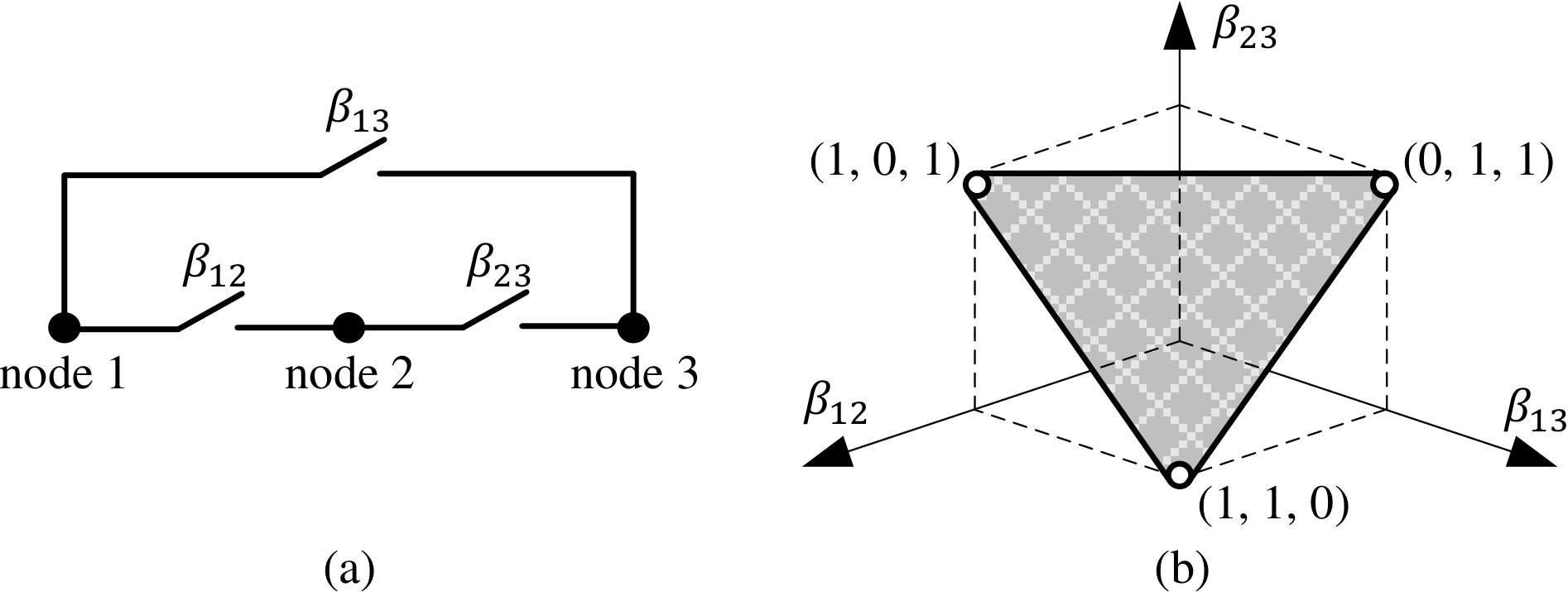 Figure 13
|
|
|
|
||||||||
|
Yes | ||||||||||
|
|
||||||||||
|
No | ||||||||||
|
|
||||||||||
|
|
|
|
| Parameters | |||
|---|---|---|---|
| Set of all DS nodes/branches. | |||
| Index for the substation node. | |||
| Variables | |||
| Flow of commodity from node to node . | |||
|
|||
|
|||
| Parameters | ||
|---|---|---|
| Set of substation nodes/DG nodes. | ||
| Set of nodes with faulted open/closed load switches. | ||
| Set of faulted open/closed branches. | ||
| Real/reactive power demand of the load at node . | ||
|
||
|
||
| Resistance/reactance/apparent power capacity of branch . | ||
| Priority weight of the load at node . | ||
| Number of branches starting or ending with node . | ||
| A large enough positive number. | ||
| Variables | ||
|
||
| Binary, if node is energized, otherwise. | ||
| Binary, is branch is closed, if open. | ||
|
||
| Squared voltage magnitude of node . | ||
| Real/reactive power flow on branch . | ||
| ——— | Model in [18] | Model in [19] | Proposed model | ||||||
|
Radial |
|
|
||||||
|
—— |
|
|
||||||
|
|
|
Flexible | ||||||
| Number of MGs | Fixed | Fixed | Flexible | ||||||
|
Not allowed | Not allowed | Allowed | ||||||
|
|
|
Flexible |
| Avg. | Avg. | Number of cases with: | ||||||
|---|---|---|---|---|---|---|---|---|
| 0.49 s | 0.56 s | 8911/10000 | 0/10000 | 1089/10000 | ||||
| Avg. | Avg. | Number of cases with: | ||||||
| 407 | 143 | 402/10000 | 21/10000 | 9577/10000 | ||||
|
||||||||
| Avg. | Avg. | Number of cases with: | ||||||
|---|---|---|---|---|---|---|---|---|
| 1.79 s | 1.54 s | 7348/10000 | 0/10000 | 2652/10000 | ||||
| Avg. | Avg. | Number of cases with: | ||||||
| 496 | 71 | 108/10000 | 134/10000 | 9758/10000 | ||||
|
||||||||
Peer Reviews
No public reviews on file for this paper yet. If you reviewed it on a platform where reviews are public (OpenReview, ICLR, NeurIPS, ICML), you can paste yours below so the community can read it here.
Videos
No videos yet. Explain this paper in a talk, walkthrough, or lecture? Add one.
Radiality Constraints for Resilient Reconfiguration of Distribution Systems:
Formulation and Application to Microgrid Formation
Shunbo Lei, Chen Chen, Yue Song, and Yunhe Hou The work of Y. Song and Y. Hou was supported in part by the Research Grant Council of Hong Kong through the Theme-based Research Scheme under Project No. T23-701/14-N. The work of Y. Hou was also supported in part by the National Natural Science Foundation of China under Grant 51677160, and in part by the Research Grant Council of Hong Kong under Grant GRF17207818.S. Lei is with the Department of Electrical Engineering and Computer Science, University of Michigan, Ann Arbor, MI 48109 USA; C. Chen is with the Energy Systems Division, Argonne National Laboratory, Argonne, IL 60439 USA; Y. Song and Y. Hou are with the Department of Electrical and Electronic Engineering, The University of Hong Kong, Hong Kong; Y. Hou is also with The University of Hong Kong Shenzhen Institute of Research and Innovation, Shenzhen 518027 China (e-mail: [email protected]; [email protected]; [email protected]; [email protected]).
Abstract
Network reconfiguration is an effective strategy for different purposes of distribution systems (DSs), e.g., resilience enhancement. In particular, DS automation, distributed generation integration and microgrid (MG) technology development, etc., are empowering much more flexible reconfiguration and operation of the system, e.g., DSs or MGs with flexible boundaries. However, the formulation of DS reconfiguration-related optimization problems to include those new flexibilities is non-trivial, especially for the issue of topology, which has to be radial. That is, the existing methods of formulating the radiality constraints can cause under-utilization of DS flexibilities. Thus, in this work, we propose a new method for radiality constraints formulation that fully enables the topological and some other related flexibilities of DSs, so that the reconfiguration-related optimization problems can have extended feasibility and enhanced optimality. Graph-theoretic supports are provided to certify its theoretical validity. As integer variables are involved, we also analyze the issues of tightness and compactness. The proposed radiality constraints are specifically applied to post-disaster MG formation, which is involved in many DS resilience-oriented service restoration and/or infrastructure recovery problems. The resulting new MG formation model, which allows more flexible merge and/or separation of the sub-grids, etc., establishes superiority over the models in the literature. Demonstrative case studies are conducted on two test systems.
Index Terms:
Distribution system, radiality constraints, reconfiguration, microgrid, resilience.
I Introduction
Distribution system (DS) reconfiguration is an effective and multi-function strategy [1, 2, 3]. Its optimization thus has been extensively studied. As most DSs have to operate with a radial topology, the mathematical formulation of radiality constraints has been specifically investigated [4, 5, 6, 7, 8] (see more details in Section III). This issue is resolved for conventional DS reconfiguration. Nevertheless, now DSs can adopt much more adaptive reconfiguration and operation owing to the added flexibilities of automation equipment, distributed generations (DGs), and microgrid (MG) components, etc. In particular, regarding the topology issue, DSs and MGs now can have flexible boundaries [9, 10, 11]. For example, the DS is split into a to-be-optimized number of MGs in [11]. Such added flexibilities are actually empowering more resilient reconfiguration of DSs.
However, existing methods to formulate radiality constraints cannot fully include those new flexibilities in optimizing DS reconfiguration [12]. That is, the feasible region given by these formulations only refers to a subset of the actual one. DS flexibilities thus will be underutilized and less coordinated, which is especially adverse for resilience-oriented reconfiguration [13]. For example, post-disaster reconfiguration is faced with quite limited flexibilities due to many faults caused by an extreme weather event [14], etc. In such cases, the faults also complicates decision-making and even requires co-optimization with other recovery efforts [15], etc. Actually, to co-optimize with the repairing sequence of the damaged parts involves reconfiguring a DS network with a physical structure evolving with the repairing variables. Existing methods to formulate radiality constraints cannot properly handle these situations.
This work proposes a new formulation of radiality constraints that fully enables topological and some other related flexibilities in DS reconfiguration-related optimization problems. It is superior to the literature’s other attempts with the same or similar aims [12] [16] (see comparisons in Section II). Graph-theoretic justifications are provided to affirm the analytical validity of it. As integer variables are involved, the tightness and compactness issues are also analyzed [17]. Generally, adopting the proposed radiality constraints in DS reconfiguration optimization problems can attain extended feasibility and enhanced optimality.
For verification, the proposed radiality constraints are applied to construct a new optimization model for post-disaster MG formation, which reconfigures the DS to form MGs energized by DGs and/or other power sources. It is an essential strategy for many resilience-oriented DS restoration and/or recovery problems [15, 16, 14, 12, 13]. Our proposed model again establishes superiority over the literature’s two groups of MG formation models [18] [19]. As compared in Fig. 1, while their models exclude some DS flexibilities, our model allows more flexible merge and separation of sub-grids, etc. (See more details in Section IV.)
In the following, Section II details the proposed method of formulating radiality constraints. Section III analyzes its tightness and compactness issues. Sections IV and V apply it to resilient MG formation. Section VI provides the conclusion.
II Proposed Radiality Constraints
This work proposes to construct radiality constraints based on two simple graph-theoretic concepts and their relationships.
First, the definition of spanning tree, which may be already well-known, is still given here to make this paper self-contained:
Definition 1
A spanning tree is a graph that connects all the vertices and contains no cycles [20].
Second, spanning forest, the other involved concept which is less common, is defined as follows:
Definition 2
A spanning forest is a graph with no cycles [20].
As in Fig. 2, a spanning forest is a graph whose connected components are spanning trees. Actually, a spanning forest with components can be called as a -tree. For example, Fig. 2(b) is a -tree. And, a -tree is a spanning tree, e.g., Fig. 2(a). Obviously, both spanning trees and spanning forests are radial.
Let be the number of substations in the DS. In light of Definitions 1 and 2, we can observe that normal DS reconfiguration for loss reduction [1] and supply capacity improvement [2], etc., is essentially forming a -tree. That is, a spanning tree is formed if , while a spanning forest is formed if . It is also required that each component has a substation node.
Regarding resilient DS reconfiguration (e.g., MG formation for service restoration), it is to form a -tree with . In this case, it is required that each component has at most one substation node, if any. Actually, the value of should be optimized in resilient reconfiguration. If it is predefined, the optimality can be impacted. In all relevant cases, we will have , which indicates that a spanning forest is formed. That is, the topology issues in resilient DS reconfiguration can be resolved by requiring the network to be a spanning forest. Thus, we can formulate the radiality constraints as equations (1)-(2), which are inspired by the remark as below:
Remark 1
An arbitrary subgraph of a spanning tree is a spanning forest.
Specifically, a subgraph of a graph consists of a subset of the vertices and edges in the graph. For example, Fig. 2(b) is a subgraph of the graph in Fig. 2(a). According to Definitions 1 and 2, Remark 1 is naturally true. Based on that, the proposed radiality constraints are formulated as follows:
[TABLE]
[TABLE]
In (1)-(2), is the set of DS branches; , where is the connection status of branch ( if closed, [math] if open); , where is the fictitious connection status of branch ( if closed, [math] if open). By “fictitious”, it indicates that are just auxiliary variables, which do not actually determine the network topology of the DS. The topology is still determined by variables . The symbol is the set of all incidence vectors of spanning tree topologies that the network can form via reconfiguration (see Section III).
Thus, constraint (1) enforces to form a fictitious spanning tree. Constraint (2) then restricts the DS to close a subset of the closed branches in the spanning tree determined by . That is, form a subgraph of the fictitious spanning tree. Remark 1 indicates that the resulting network topology determined by is a spanning forest. Note that constraint (1) is just expressed conceptually here. We will elaborate on its explicit formulations in Section III. Besides, constraints (1)-(2) implicitly assume that the DS has only one substation node. Section III will briefly explain the reason for this assumption, and introduce a simple method that enables the proposed radiality constraints to fully handle a DS with multiple substation nodes. For uncontrollable branches without switches or with faulted switches, constraints can be added to specify their connection status (see Section IV).
Remark 1 only specifies that any satisfying constraints (1)-(2) is topologically feasible for the DS. The following theorem indicates that any topologically feasible satisfies constraints (1)-(2). As it is somewhat less straightforward, its proof is also provided. Remark 1 and Theorem 1 together certify the validity of the proposed radiality constraints.
Theorem 1
A spanning forest subgraph of a connected graph is also the subgraph of a spanning tree subgraph of the connected graph.
Proof: Assume a -tree denoted as to be a subgraph of a graph . As is connected, there exists at least one edge in that can link the th component of to another component of . Adding this edge to , which does not create cycles, becomes a -tree denoted as . Repeating this process, ends up to be a -tree denoted as . Obviously, the spanning forest is a subgraph of the spanning tree , which is a subgraph of . This completes the proof.
The proposed radiality constraints (1)-(2) can be interpreted as a two-step method to regulate DS topology in reconfiguration. In the first step, constraint (1) ensures network radiality by having a spanning tree to be the DS topology’s supergraph, which is determined by the fictitious connection status of branches. (If is a subgraph of , then is said to be a supergraph of .) In the second step, constraint (2) enables more flexible reconfiguration by allowing the DS to select a subgraph of the fictitious spanning tree to be the actual network topology.
By contrast, common methods of formulating radiality constraints in the literature (e.g., [6] [8]) can be seen as a one-step process that directly enforces the DS topology to be a spanning tree or a spanning forest. Their models (the single-commodity flow model [6], etc.) can also be used to formulate constraint (1) here. Nevertheless, a new formulation will be presented in Section III. Above all, the proposed two-step method for radiality constraints formulation enables many more flexibilities in DS reconfiguration, such as more adaptive merge or separation of sub-grids, and more flexible allocation of power sources into sub-grids. Such benefits will be detailed in Sections IV and V applying the proposed radiality constraints to resilient MG formation.
Due to the critical importance of network reconfiguration in DS resilience enhancement, etc., many publications also propose to develop new methods of ensuring radiality to allow undiminished flexibilities and adaptivities of DSs in optimization. Specifically, references [12][16] have presented two applicable methods, which are compared to our proposed method as below:
II-1 Validity
Remark 1 and Theorem 1 theoretically prove the validity of constraints (1)-(2) here. References [12] [16] however lack such analytical proofs for their proposed formulations.
II-2 Tightness
With constraint (1) properly formulated, our proposed model attains the tightest formulation of the spanning forest polytope of the DS, i.e., the convex hull of incidence vectors of possible spanning forest topologies (see Section III). The methods in [12] [16] produce relatively less tight formulations.
II-3 Compactness
Constraint (1) can also be formulated in less tight but more compact manners (see Section III). In this regard, the resulting topology constraints (1)-(2) are generally more compact than (i.e., with fewer variables and constraints), and still as tight as or even tighter than those of [12] [16].
II-4 Application convenience
The application of our proposed method can be quite straightforward, i.e., simply adding constraint (2) to the commonly-used single-commodity flow-based radiality constraints. The methods in [12] [16] however involve the introduction of a virtual source node and virtual branches, and the modeling of a virtual DC optimal power flow subproblem and its Karush-Kuhn-Tucker conditions etc., respectively.
II-5 Applicability
The proposed radiality constraints (1)-(2) can be adopted in different DS optimization problems involving reconfiguration. Topological and some other related flexibilities thus can be fully enabled in optimization. The methods in [12] [16] have some limitations in this regard. For example, the radiality constraints proposed in [12] allow the merge of sub-grids in optimization, but do not enable their possible separation.
III Tightness and Compactness Issues
Constraint (1) is only expressed conceptually in Section II. As aforementioned, common methods or models for representing radiality constraints in DS reconfiguration-related publications can be used for its explicit formulation. Those methods and models are revisited here. A new model is also presented. The tightness and compactness issues are specifically discussed.
DS reconfiguration is essentially a mixed-integer programming (MIP) problem generally solved by the branch-and-cut (B&C) method, which needs to solve its linear programming (LP) relaxations (i.e., relaxing integerbinary constraints). The computational complexity of a MIP depends on its tightness and compactness, etc. A MIP formulation is tight if its feasible region is similar to that of its LP relaxation, contributing to a smaller gap between the optimal values (solutions) of the MIP and its LP relaxation, and less explored nodes in the B&C search tree (i.e., fewer iterations and faster convergence). A compact MIP formulation has a small number of variables and constraints, leading to shorter computation time for each explored node in the B&C search tree. Tightness and compactness are often conflicting objectives in formulating a MIP [17].
Several relevant concepts are further introduced. Here, incidence vectors of spanning trees are values of defining fictitious spanning tree topologies of the DS; and spanning tree polytope is the convex hull of such incidence vectors. For example, the system in Fig. 3(a) has . Its incidence vectors of spanning trees include , and , and its spanning tree polytope is the shaded region with those vectors as the vertices in Fig. 3(b). Incidence vectors of spanning forests and spanning forest polytope are defined likewise.
That is, constraint (1) actually requires to be an incidence vector of a spanning tree. A tight and compact formulation is desired to explicitly represent this requirement. LP relaxations of the tightest formulations define the spanning tree polytope.
Some methods or models to express radiality constraints in DS reconfiguration-related publications can be used to formulate the spanning tree constraint (1). They are revisited here:
III-1 Loop-eliminating method [4]
It enumerates all loops of the DS, and enforces each one to be open. However, finding all loops in a graph is NP-hard. This method is essentially equivalent to the subtour elimination formulation of spanning tree constraints in graph theory. As one of the tightest formulations, its LP relaxation defines the spanning tree polytope and thus has integer extreme points. It has only variables but also an exponential number of constraints, which limits its application.
III-2 Path-based model [5]
It enumerates all paths to the substation for each node, and activates only one of them. Still, finding all paths between two graph nodes is NP-hard. This model also has a counterpart in graph theory, i.e., the directed cutset formulation of spanning tree constraints with 3$$\cdot$$|\boldsymbol{L}| variables and an exponential number of constraints. It is one of the tightest formulations with integer vertices of its LP relaxation, too.
III-3 Single-commodity flow-based model [6]
It closes |\boldsymbol{N}|$$-$$1 branches (: set of DS nodes), and ensures connectivity by imposing unit fictitious flow from the substation to each node. With 3$$\cdot$$|\boldsymbol{L}| (or reduced to 2$$\cdot$$|\boldsymbol{L}|) variables and a linear number of constraints, it is one of the most compact formulations. Due to its simplicity, it is also the most commonly used DS radiality model. Still, it is less tight. The projection of its LP relaxation into the -space defines a region larger than the spanning tree polytope, and therefore has fractional extreme points.
III-4 Parent-child relation-based method [7]
It instructs every node except the substation to have one parent. However, this method can produce a disconnected graph with loops [8].
III-5 Primal and dual graphs-based model [8]
It froces each primal (dual) node to be connected to another primal (dual) node, and forbids the primal and dual spanning trees to be intersected. With 4$$\cdot$$|\boldsymbol{L}| variables and a linear number of constraints, it is one of the most compact formulations. Originally proposed in [22], it actually has a totally unimodular constraint matrix to define a polyhedron with integer vertices. Thus, it is also one of the tightest formulations with its LP relaxation defining the spanning tree polytope in the -space. Still, it is only applicable to planar graphs, and needs to construct dual graphs. It also has a flaw to be avoided by appropriate selection of roots [23]. Generally, its applicability is limited and its use is not convenient.
Using notations in Table II, we further introduce a new flow-based formulation of the spanning tree constraint (1) as below:
[TABLE]
[TABLE]
[TABLE]
[TABLE]
[TABLE]
[TABLE]
[TABLE]
The above formulation is called as the directed multicommodity flow-based model of the spanning tree constraints. It defines a fictitious commodity for each node , and enforces 1 unit of commodity delivered from the substation node to node . Constraint (6) implies that each commodity can flow on an arc only if the arc is included in the directed spanning tree defined by variables . Other equations are self-explanatory.
The LP relaxation of the above formulation (3)-(9) defines the spanning tree polytope (i.e., ) in the -space by a polynomial number of variables and constraints. As compared in Table I, it is generally the most compact formulation among the ones that are the tightest and applicable for both planar and non-planar graphs. Now the models listed in Table I actually cover a wide spectrum of tightness and compactness levels for the formulation of spanning tree constraints. Researchers and practitioners may choose an appropriate model based on their preferences and needs, etc.
Next, the tightness and compactness of constraints (1)-(2), rather than solely constraint (1), are further discussed briefly.
Proposition 1
If the LP relaxation of the explicit formulation of constraint (1) defines the spanning tree polytope in the -space, the LP relaxation of the proposed radiality constraints (1)-(2) defines the spanning forest polytope in the -space.
Proof: Assume that the LP relaxation of constraints (1)-(2) has a fractional vertex in the -space. Further assume that has fractional entries. Thus, can be represented by an integer vertex and another point of the spanning tree polytope: with . For with or , we have and , respectively. As and , we have for with , and have with for with . Then, we can construct and to have and for with , and have and for with , so that . This contradicts the assumption of being a vertex. The case with as a vertex of can be analyzed similarly. Thus, vertices of the projection of constraints (1)-(2)’s LP relaxation into -space are 0-1 incidence vectors of spanning forests of the DS.
Proposition 1 implies that the tightness and compactness features of constraints (1)-(2) essentially follow the explicit formulation of constraint (1). Thus, the proposed radiality constraints (1)-(2) also cover a wide spectrum of tightness and compactness levels for the formulation of spanning forest polytope. An appropriate model can be selected based on one’s preferences, etc.
Specifically, to exploit the aforementioned properties of the formulations, the DS is assumed to have only one substation node. For a DS with multiple substation nodes, one can merge them into one node in modeling constraints (1)-(2), but still treat them as separate nodes in modeling DS operational constraints.
IV Application to Resilient MG Formation
The proposed radiality model (1)-(2) can be applied in different optimization problems involving DSs and/or MGs with flexible boundaries [9, 10, 11], etc. Here, we apply it to regulate the DS topology in resilient MG formation to verify its advantages.
MG formation has recently been extensively studied in [13] [18] [19] [24] [25], etc. It is to reconfigure the DS into multiple MGs energized by DGs, so as to restore critical loads, etc. The literature currently has two major types of optimization models for this problem [18] [19]. Using the proposed radiality model, a new formulation for resilient MG formation is constructed:
[TABLE]
[TABLE]
[TABLE]
[TABLE]
[TABLE]
[TABLE]
[TABLE]
[TABLE]
[TABLE]
[TABLE]
[TABLE]
[TABLE]
[TABLE]
Notations are listed in Table III. The objective function (10) maximizes the weighted sum of restored loads. Constraints (1)-(2) are used to ensure radiality and enable topological flexibilities, etc. Constraint (1) is formulated using the methods in Section III. Equations (11)-(12) enforce real and reactive power balance, respectively. Equation (13) imposes zero power output for nodes without power sources. Constraint (14) indicates real and reactive power capacities of substations or DGs. Constraint (15) represents the DistFlow model with the much smaller quadratic terms ignored [1] [26]. It is relaxed for open branches. Constraint (16) expresses the voltage magnitude limits. Constraint (17) is convex though non-linear, and can be linearized by the technique in [3], etc. It limits the apparent power on a branch by its capacity. Equation (18) restricts the connection status of faulted open or faulted closed branches. Equation (19) prohibits picking up the loads with faulted open switches, and enforces picking up the loads with faulted closed switches as long as their located nodes are energized. Equation (20) specifies that substation and DG nodes are energized. Constraint (21) derives the energization status of other nodes by examining if they are connected to an energized node. The non-linear and non-convex terms, i.e., and , can be equivalently linearized and convexified by the McCormick envelopes [27].
Note that the areas with surviving access to the main grid power via substation nodes are also considered. Operational constraints may prohibit those areas to be fully restored by the substations, and forming MGs with DGs can help achieve better restoration of them [14]. For statement simplicity, a sub-grid powered by a substation is also counted as a MG here.
Table IV compares the proposed model with the two existing MG formation models in the literature. The summaries in the table are self-explanatory. Brief explanations are given as below:
-
The model in [18] is designed for radial systems. It is extended in [25] to deal with meshed systems. Still, the extended model does not eliminate loops. Thus, it may be used for the bulk power system, but does not apply to meshed DSs, which have to open some branches to be operated in radial topologies. Both model in [19] and our model can handle meshed DSs, as radiality constraints are included to avoid loops when reconfiguring the network. Single-commodity flow-based radiality constraints are used in[19], while our model adopts the proposed radiality constraints to fully enable topological flexibilities, etc.
-
Both models in [18] and [19] allocate one DG to each MG. Therefore, the number of MGs is actually fixed and equal to the number of DGs and/or other power sources. As for our proposed model, the number of DGs designated to different MGs, and the resulting number of MGs, are flexible. Thus, it can also be used for dynamic MG formation, which involves adaptive merge and/or separation of MGs when damaged parts of the DS are sequentially repaired, etc. Such flexibilities introduce many benefits. For example, larger MGs can be formed to better match DGs with different-sized loads, so as to enhance capacity utilization rates of DGs and the restoration of critical loads.
-
Both models in [18] [19] energize all nodes included in . Thus, their models cannot consider the nodes in load islands without power sources and isolated by faulted open branches. Discrete/non-dispatchable loads at nodes are also forced to be picked up in their models. Our model can consider such load islands, and can be easily extended to optimize the allocation of mobile power sources in such islands and their merge with other islands after faulted open branches are repaired. Our model can also intentionally form unenergized islands in optimization, enabling more flexible pick-up of the loads at nodes . This flexibility can be critical, as some DSs may have a large portion of loads not equipped with switches, causing to be a large set. In [13], with additional binary variables, the model in [19] is modified to permit more flexible allocation of DGs into MGs. However, it does not fully enable topological and some related flexibilities. For example, it still requires energizing all nodes.
In general, as indicated in Table IV, the proposed MG formation model is more adaptive and allows more flexibilities.
V Case Studies
In this section, the proposed resilient MG formation model is demonstrated on two test systems. We use a computer with an Intel i5-4278U processor and 8GB of memory. Involved MIP problems are solved by Gurobi 7.5.2 with the default settings.
V-A IEEE 33-Node Test System [1]
Fig. 4 depicts an illustrative case based on a scenario with 27
faults in total. The model in [18] does not apply to meshed DSs. Thus, as indicated in Fig. 4(a), it does not consider the normally open branches. It forms 6 MGs energized by the 6 DGs, respectively. As the model in [19] can handle meshed DSs, it gets better results via further reconfiguration involving those normally open switches, etc. Fig. 4(b) shows that it restores more loads by forming 6 larger MGs, which is essentially a 6-tree. By contrast, as in Fig. 4(c), our proposed model forms a 7-tree, i.e., 4 MGs and 3 load islands. Specifically, MG 4 and MG 6 in Fig. 4(b) are merged into a single MG in Fig. 4(c), so that the loads at nodes 31 and 33 can also be restored. MG 2 in Fig. 4(b) is separated into a MG and a load island in Fig. 4(c), so that node 23 is not energized and its load is not forced to be picked up. For space limit, we do not detail on other differences. The models in [18] [19] and our proposed model have DG capacity utilization rates of 55.6%, 67.4% and 95.4%, respectively. They restore 1500kW, 1820kW and 2575kW loads, respectively. Our model achieves more coordinated matching among the different-sized DGs and loads, and thus attains better service restoration. Generally, as the proposed radiality constraints can fully enable topological and some other related flexibilities of the DS, our MG formation model has extended feasibility and enhanced optimality.
To establish superiority of the proposed radiality constraints and MG formation model, we further run 10000 cases based on randomly generated scenarios of DS faults. Table V shows that our model has far less infeasible cases. In many scenarios, it finds a feasible operating point of the DS, while the models in [18] [19] return infeasibility. Such results verify that our model has extended feasibility as the proposed radiality constraints fully enable topological and some related flexibilities. Besides, while its search space is the largest, its average computation time is the shortest. Thus, its enlarged feasible set may possess more computationally tractable characteritics. As in Table VI, our model has the highest average/median/minimum restored loads and the smallest standard deviation. The same maximum value corresponds to the cases with all loads restored. On average, the proposed model restores 15.0% and 8.4% more loads than models in [18] and [19], respectively. Actually, our model performs equally well or better in all cases. The histograms in Fig. 5(Left) depict the outperformance. Such results validate the enhanced optimality of the proposed model. Here, one of the major reasons for its superiority is more coordinated matching among the DGs and loads. Table VII indicates that the average DG capacity utilization rate of our model is much higher than those of the models in [18] [19]. The smaller minimum and larger standard deviation are due to the cases with the substation contributing much power injection for service restoration.
The single-commodity flow-based model is used to formulate constraint (1) in all previous cases. Here, for comparison, the directed multicommodity flow-based model is used instead. Consequently, the proposed radiality constraints and MG formation model become tighter, though less compact. The revised model is run on the same 10000 scenarios. As indicated in Table VIII, is much smaller than , both on average and in 95.8% of the cases. The histogram in Fig. 5(Right) also details the extra explored nodes in the B&C search tree of the less tight model. Although is slightly shorter than on average, is much shorter than in 10.9% cases. Specifically, in those cases, and are 1.92 s and 0.69 s on average, respectively; and are 815 and 186 on average, respectively. In general, the computation time of the revised tighter model is more consistent. It also reduces the computation time in many cases that require the less tight model to explore much more nodes in the B&C search tree. That is, the proposed radiality constraints can satisfy the need for tighter formulations of DS reconfiguration-related optimization problems.
V-B IEEE 123-Node Test System [28]
Fig. 6 provides an illustrative case based on a 60-fault sce-
nario using the proposed MG formation model. It forms 7 MGs powered by 8 DGs, and a sub-grid powered by the substation. The DG capacity utilization rate is 75.0%, and 3730kW loads are restored. We again run 10000 cases on random scenarios of DS faults. Table IX-XII and Fig. 7 show results similar to the previous system. That is, the proposed radiality constraints and MG formation model’s superiority is also established on this larger system. For example, our model matches DGs and loads in a more coordinated manner, thus achieving better service restoration. For space limit, we do not go into the details. In short, our MG formation model has extended feasibility and enhanced optimality due to the proposed radiality constraints’ fully enabling topological and some related flexibilities of DSs.
It is worth mentioning that, as in Table XII, is averagely shorter than for this larger system. Specifically, in the cases with , and are 1.26 s and 5.59 s on average, respectively; and are 89 and 937 on average, respectively. That is, the computation time of the tighter version of our MG formation model is not only shorter on average, but also more consistent. It greatly reduces the computation time especially for cases requiring the less tight model to explore much more B&C search tree nodes. Thus, the tighter version of the proposed radiality constraints can allow both more flexible DS operation and more efficient computation for reconfiguration-related optimization problems, e.g., MG formation here.
VI Conclusion
This work proposes a new method for formulating radiality constraints that fully enables topological and some other related flexibilities in DS reconfiguration optimization problems. It is specifically applied to resilient post-disaster MG formation to attain extended feasibility and enhanced optimality. As verified in case studies, compared to the existing MG formation models, our model based on the proposed radiality constraints achieves a higher resilience enhancement via more coordinated utilization of DS flexibilities, etc., and reduces the computational complexity. Future work includes exploring the effects of increased topological flexibilities on other DS performance metrics, etc.
The reference list from the paper itself. Each links out to its DOI / PubMed record.
- 1[1] M. E. Baran and F. F. Wu, “Network reconfiguration in distribution systems for loss reduction and load balancing,” IEEE Trans. Power Del. , vol. 4, no. 2, pp. 1401–1407, Apr. 1989.
- 2[2] K. Chen, W. Wu, B. Zhang, S. Djokic, and G. P. Harrison, “A method to evaluate total supply capability of distribution systems considering network reconfiguration and daily load curves,” IEEE Trans. Power Syst. , vol. 31, no. 3, pp. 2096–2104, May 2016.
- 3[3] X. Chen, W. Wu, and B. Zhang, “Robust restoration method for active distribution networks,” IEEE Trans. Power Syst. , vol. 31, no. 5, pp. 4005–4015, Sep. 2016.
- 4[4] J.-Y. Fan, L. Zhang, and J. D. Mc Donald, “Distribution network reconfiguration: single loop optimization,” IEEE Trans. Power Syst. , vol. 11, no. 3, pp. 1643–1647, Aug. 1996.
- 5[5] E. R. Ramos, A. G. Expósito, J. R. Santos, and F. L. Iborra, “Path-based distribution network modeling: application to reconfiguration for loss reduction,” IEEE Trans. Power Syst. , vol. 20, no. 2, pp. 556–564, May 2005.
- 6[6] M. Lavorato, J. F. Franco, M. J. Rider, and R. Romero, “Imposing radiality constraints in distribution system optimization problems,” IEEE Trans. Power Syst. , vol. 27, no. 1, pp. 172–180, Feb. 2012.
- 7[7] R. A. Jabr, R. Singh, and B. C. Pal, “Minimum loss network reconfiguration using mixed-integer convex programming,” IEEE Trans. Power Syst. , vol. 27, no. 2, pp. 1106–1115, May 2012.
- 8[8] H. Ahmadi and J. R. Martí, “Mathematical representation of radiality constraint in distribution system reconfiguration problem,” Int. J. Electr. Power Energy Syst , vol. 64, pp. 293–299, Jan. 2015.