Exponential stability for the nonlinear Schr\"odinger equation on a star-shaped network
Ka\"is Ammari, Ahmed Bchatnia, Naima Mehenaoui

TL;DR
This paper proves that solutions to a nonlinear dissipative Schr"odinger equation on a star-shaped network decay exponentially over time, with damping localized on one branch and at infinity.
Contribution
It establishes exponential stability for the nonlinear Schr"odinger equation on a star-shaped network with localized damping, a novel result in this setting.
Findings
Exponential decay of solutions proven
Stability holds with damping on one branch and at infinity
Advances understanding of nonlinear Schr"odinger dynamics on networks
Abstract
In this paper, we prove the exponential stability of the solution of the nonlinear dissipative Schr\"odinger equation on a star-shaped network and where the damping is localized on one branch and at the infinity.
Click any figure to enlarge with its caption.
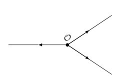 Figure 1
Peer Reviews
No public reviews on file for this paper yet. If you reviewed it on a platform where reviews are public (OpenReview, ICLR, NeurIPS, ICML), you can paste yours below so the community can read it here.
Videos
No videos yet. Explain this paper in a talk, walkthrough, or lecture? Add one.
Exponential stability for the nonlinear Schrödinger equation on a star-shaped network
Kaïs Ammari
UR Analysis and Control of PDEs, UR13ES64, Department of Mathematics, Faculty of Sciences of Monastir, University of Monastir, 5019 Monastir, Tunisia
,
Ahmed Bchatnia
UR Analyse non-linéaire et géométrie, UR13ES32, Department of Mathematics, Faculty of Sciences of Tunis, University of Tunis El-Manar, 2092 El Manar II, Tunisia
and
Naima Mehenaoui
Department of Mathematics, Faculty of Sciences of Tunis, University of Tunis El-Manar, 2092 El Manar II, Tunisia
Abstract.
In this paper, we prove the exponential stability of the solution of the nonlinear dissipative Schrödinger equation on a star-shaped network and where the damping is localized on one branch and at the infinity.
Key words and phrases:
Exponential stability, dissipative Schrödinger equation, star-shaped network
2010 Mathematics Subject Classification:
35L05, 34K35
Contents
1. Introduction
Dispersive models have long been a question of great interest in a wide range of researchers. One of the most significant current discussions in these models is the nonlinear Schrödinger equation. This equation has been studied extensively since the early years of this century. Most of these studies have mainly concentrated on the well-posedness questions, see, for instance [6] and stabilization of the energy. The author in [9, 10] established an exponential decay rate of the energy in -level for the nonlinear Schrödinger equation with localized damping.
In this paper, we derive analogous exponential decay rate in -level for the nonlinear dissipative Schrödinger equation on a star-shaped network, as in Figure 1, and where the damping is localized on one branch and at the infinity. More precisely we consider the following initial and boundary-value problem:
[TABLE]
where and will be treated in this paper. The presence of the damping term in (1.1) is responsible for the localized mechanism of dissipation of the system since the function is assumed to be in , almost everywhere non-negative function, and to satisfy for some , and ,
[TABLE]
The considered graph consists of a finite number of edges of infinite length attached to a common vertex, each of them being identified with a copy of the positive semi-axis. In the context of nonlinear Schrödinger equation on a star-shaped network, Ali Mehmeti, Ammari and Nicaise in [2] have proved -time decay estimates. Banica and Ignat in [3] proved the same results in the case of trees with the last generation of edges of infinite strips, with Kirchhoff coupling condition at the vertices. With the same conditions, dispersive estimates were obtained in the case of the tadpole graph in [1]. The motivation for studying nonlinear propagation in ramified structures comes from several branches of pure and applied science, modeling phenomena such as nonlinear electromagnetic pulse propagation in optical fibers, the hydrodynamic flow, electrical signal propagation in the nervous system, etc.
Before a precise statement of our main results, let us introduce some definitions and notations about 1-d networks which will be used throughout the rest of the paper.
Let , be disjoint sets identified with to . We set . We denote by the functions on taking their values in and let be the restriction of to .
Define the Hilbert space with inner product
[TABLE]
The energy identity obtained from , by simple formal calculations, is given by
[TABLE]
[TABLE]
where and is the energy of , defined by
Our major concern will be to prove the exponential decay of the global energy at the infinity. More precisely we have the following theorem:
Theorem 1.1**.**
Consider , a function satisfying assumption (1.2) and the initial data in . For any solution of the system (1.1), there exist and such that:
[TABLE]
provided the initial data satisfies if one considers the case
The paper is organized as follows. In Section 2, we prove that the system (1.1) is globally well-posed in the energy space . Section 3 is devoted to the proof of the main result. Technical results are collected in the appendix.
2. Well-posedness
In this section, we show the global well-posedness in of the problem for initial data in , by combining the techniques due to Kato, established in [4] and [7]. We first recall the following Strichartz estimates, see [4, 7] for more details.
Theorem 2.1**.**
The group associated to the Schrödinger equation satisfies the following properties:
** 2. 2)
** 3. 3)
**
In all cases, we have and
[TABLE]
Here, constant depends only on .
As a consequence we have the following (see [4] and [7]).
Corollary 2.2**.**
Consider and two pairs of constants satisfying condition . One has
[TABLE]
where
We have under the assumption (1.2) the following local well-posedness result in -level for the nonlinear Schrödinger :
Theorem 2.3**.**
Given and , then there exist and a unique solution of system (1.1) such that:
[TABLE]
where
Proof.
We divide the proof in two cases.
Consider and positive constants, we need to construct the complete metric space,
[TABLE]
where indicates the natural norm of the space
[TABLE]
given by:
[TABLE]
for .
Step 1. Define, for any
[TABLE]
By using Theorem 2.1, we deduce from the definition in equation 2.4 and Corollary 2.2 that
[TABLE]
where . Hölder’s inequality gives
[TABLE]
where , and .
So, if , where , we have
[TABLE]
Then, we have
[TABLE]
where .
Similarly, we have
[TABLE]
where the positive constant depends on , and the norm of the function . Then, from equation and , we have
[TABLE]
We fixe Inequality enable us to deduce
[TABLE]
So, by choosing , such that
[TABLE]
we get
[TABLE]
It follows that is well-defined on , that is .
Step 2. Now, if , we have
[TABLE]
The same argument as in , show that
[TABLE]
Since then by Hölder’s inequality, we obtain that
[TABLE]
So, we have
[TABLE]
where . Similarly, we have
[TABLE]
[TABLE]
Combining and , we obtain
[TABLE]
It follows from the choice of , and inequality
[TABLE]
So, is a contraction from into itself, then we have proved the existence and uniqueness of the solution of the problem
[TABLE]
Step 3. Note that if are the corresponding solutions of (2.17) with initial data , respectively, then
[TABLE]
Similarly, following the same arguments used earlier, we get
[TABLE]
where Analogously, we have
[TABLE]
where Combining and
[TABLE]
[TABLE]
If is small enough (see ), then
[TABLE]
Consequently, we have proved the continuous dependence of with respect to . This completes the proof of case I).
In this case, we need some modifications in the proof of case I) given above.
According to [4, 7], we have for be a pair satisfying condition in Theorem 2.1: Given and , there is and such that if
[TABLE]
then,
[TABLE]
Let us define the complete metric space
[TABLE]
where given by
[TABLE]
Step 1. Applying Theorem 2.1 and Corollary 2.2 to system , it follows that
[TABLE]
Therefore, we have
[TABLE]
where Similarly, by applying Theorem 2.1, Corollary 2.2 and the estimate to the system , we obtain
[TABLE]
Then, we have
[TABLE]
We get from and that
[TABLE]
Therefore, if
[TABLE]
we get that .
Step 2. The argument used in the proof of Theorem 2.3 yields
[TABLE]
Similarly, we have
[TABLE]
This yields,
[TABLE]
thus, for
[TABLE]
we have that is a contraction. Now, taking and , such that
[TABLE]
we see that both and are verified. This completes the proof, the remainder of the proof follows the same argument employed to show case I). ∎
We have the following result:
Corollary 2.4**.**
The solution of the system obtained in Theorem 2.3 belongs to for all admissible pair defined in Theorem 2.1.
Proof.
The proof of this results is similar to the one given in [7, Corollary 5.1] for the subcritical case and [4, Theorem 4.7.1] for the critical case. ∎
Remark 2.5*.*
Notice that the time of existence in the subcritical case depends only on ; meanwhile, in the critical case, the time of existence depends on the itself, and not only on its norm.
The following corollaries establish global solution of the system in -norm in subcritical case and critical case respectively.
Corollary 2.6**.**
If the nonlinearity power , then for any the local solution of the system extends globally with
[TABLE]
where satisfies the condition
Proof.
Since depends only on and, by using , we have , we deduce, after an interaction argument, that a similar inequality as in remains valid for all . This last fact enable us to conclude that can be extended to all ∎
The situation for the critical case is quite different. In this case, the local result shows the existence of a solution in a time interval depending on the data itself and not its norm. So, the fact that does not guarantee the existence of a global solution. An important result of global solutions for this case is established provided that is assumed a smallness condition on the initial data. According to [4, 7], we have:
Corollary 2.7**.**
Let us assume . The additional assumption implies that the local solution of the system can be extended globally, that is
[TABLE]
where are admissible pairs satisfying condition .
3. Exponential stability
First, we give the following technical lemma:
Lemma 3.1**.**
The solution related to the system (1.1) verifies the following inequality:
[TABLE]
[TABLE]
Proof.
It is clear that:
[TABLE]
Now, using the fact that , and (3.2), we obtain the desired result. ∎
Next, the following lemma is aimed to prove an estimate-type observability estimate.
Lemma 3.2**.**
Consider . Let be a solution associated to the system with initial data satisfying for the case . Then, for all there exists a positive constant which depends on such that the following inequality holds,
[TABLE]
Proof.
We argue par contradiction. We suppose that (3.3) is not true and let be a sequence of initial data attached with the solutions which is assumed to be uniformly bounded by a constant verify
[TABLE]
On account of we obtain a subsequence of , still denoted by , which verifies the convergence
[TABLE]
Then, we deduce
[TABLE]
Consequently, we have
[TABLE]
On the other hand, by using Lemma 3.1, we deduce the existence of ( for the case ) such that
[TABLE]
Now, we consider the equation
[TABLE]
First, we consider . Note that:
- •
The term is bounded in (Stricharz estimates) and
- •
Similarly, the term
- •
Since is bounded in the term is bounded in
The case is analogous. The main difficulty is to deal with the nonlinear term . By applying Theorem 2.3, Corollary 2.7 and Strichartz estimates, we have that is bounded in . the remainder of the conclusion is similar.
Thus, we deduce that is bounded in and we conclude, by using Lemma 3.6, the existence of a subsequence, still denoted by , such that
[TABLE]
Besides we have a.e. in Using (3.7) and (3.10) we get
[TABLE]
At this point, we will divide the proof into two cases.
Case 1:
First, we consider the case , handling by the Strichartz inequalities we have is bounded in for all .
Therefore, is bounded in . Consequently, we obtain in . Now, we can pass to the limit in (3.9), we find
[TABLE]
Furthermore, since there is such that and therefore Incoming, we see that is a mild solution with initial data having compact support and we use Theorem 3.3 (see appendix) to conclude that with for all Consequently, we obtain , for all and Which gives in (see Theorem 3.4 in appendix). We obtain finally in
In the sequel, we have
[TABLE]
Using estimations , we obtain
[TABLE]
[TABLE]
Using and the fact that
[TABLE]
We get
[TABLE]
Therefore, since , for all we deduce that in This gives a contradiction.
Now, we consider . The procedure is very similar. The main difference is to justify the passage to the limit at system (3.12). Handling by the Strichartz inequalities and since , we have in bounded in , for all . Therefore, is bounded in . The remainder of the proof follows similarly as determinate in the case .
Case 2:
Let .
We have, by using Lebesgue’s Dominated Convergence Theorem, that
[TABLE]
Also, satisfies and verifies:
[TABLE]
By virtue of (3.4) and (3.16) we get:
[TABLE]
Using the fact that , we deduce from (3.18):
[TABLE]
and this allow to find in L^{2}\Big{(}(0,T);L^{2}([R,+\infty[)\Big{)}. Using the same arguments as in the case , (also in this case, we need to infer a bound for the nonlinear term in , where for and for ), we conclude that , for some , is bounded in and we get a function which verifies:
- •
weakly in L^{2}\Big{(}(0,T_{2}),L^{2}(\mathbb{R}_{+})\Big{)},
- •
satisfies
[TABLE]
where is a solution of
[TABLE]
Thanks to Holmogren’s Theorem and (3.21) we obtain in On the other hand, we use the fact that is bounded in L^{2}\Big{(}(0,T_{2});H^{1/2}(0,R)\Big{)} and Aubin-Lions’s Lemma (Lemma 3.6 in appendix) to infer that:
[TABLE]
Combining (3.19) with (3.22) we get:
[TABLE]
Finally, we use the same arguments used to compute the limit in (3.15) to obtain
[TABLE]
This is in contradiction with .
∎
Now, we prove our main stability result (1.4).
Proof of Theorem 1.1.
Combining (3.1) and (3.3), we get:
[TABLE]
Using the fact that is a nonincreasing function we deduce:
[TABLE]
where C(T):=\Big{(}\frac{1}{2c}+\frac{1}{2\alpha_{0}}\Big{)}.
This implies that
[TABLE]
Finally, using the semigroup property, we obtain the exponential decay. ∎
Appendix
In this appendix, we present some useful results used in the paper. Let us first recall a result establishing a smoothing effect of nonlinear Schödinger equation.
Theorem 3.3**.**
([4, Theorem ]) Consider , and an odd positive number. Let be the global solution in C\left(\left[0,T\right];L^{2}(\mathcal{R})\right)\cap L^{2}\big{(}(0,T);L^{\infty}(\mathcal{R})\big{)} of
[TABLE]
Then, for all with a compact support.
We have the same result for star-shaped and tadpole graph geometries, see[1] and [2] respectively, for more details.
We recall also the following unique continuation theorem for regular solutions of the nonlinear equation in . This result is more general in the sense that it deserves for nonlinear Schrödinger equation in the domain , with a general nonlinearity . In such case, we must consider satisfying .
Let us define the weighted Sobolev space , as
[TABLE]
Theorem 3.4**.**
([5, Theorem 2.1]) Let , , be a strong solution of the equation in in the domain . If there is , and such that
[TABLE]
then .
Now, notice the following lemmas.
Lemma 3.5**.**
(Lions’Lemma [8, Lemma 1.3]) Let be an open bounded subset of . Consider a sequence in , , satisfying and a.e. in . Thus in , as .
Lemma 3.6**.**
(Aubin-Lions’Lemma [11, Corollary 4]) Let , and be three Banach spaces with . Suppose that is compactly embedded in and that is continuously embedded in . Suppose also that and are reflexive spaces. For , let . Then the embedding of into is compact.
The reference list from the paper itself. Each links out to its DOI / PubMed record.
- 1[1] F. Ali Mehmeti, K. Ammari and S. Nicaise, Dispersive effects for the Schrödinger equation on the tadpole graph, J. Math. Anal. Appl., 448 (2017), 262–280.
- 2[2] by same author, Dispersive effects and high frequency behaviour for the Schrödinger equation in star-shaped networks, Port. Math., 72 (2015), 309–355.
- 3[3] V. Banica and L. I. Ignat, Dispersion for the Schrödinger equation on networks, J. Math. Phys. 52 , 083703 (2011).
- 4[4] T. Cazenave, Semilinear Schrödinger Equations, Courant Lect. Notes Math., vol. 10, 2003.
- 5[5] L. Escauriaza, C. E. Kenig, G. Ponce and L. Vega, On uniqueness properties of solutions of Schrödinger equations, Comm. Partial Differential Equations, 31 (2006), 1811–1823.
- 6[6] T. Kato, On nonlinear Schrödinger equations, Ann. Inst. H. Poincaré Anal. Non Linéaire, 46 (1987), 113-–129.
- 7[7] F. Linares and G. Ponce, Introduction to Nonlinear Dispersive Equations, Springer, New York, 2009.
- 8[8] J. L. Lions, Quelques méthodes de résolution des problèmes aux limites non linéaires, Gauthier-Villars: Dunod; 1969.