TL;DR
This paper introduces probabilistic methods to improve the robustness of Natural Language Inference models against dataset biases, enhancing their transferability across different datasets.
Contribution
It proposes novel probabilistic approaches that discourage models from ignoring premises, leading to better generalization and robustness in NLI tasks.
Findings
Methods improve robustness on 9 out of 12 datasets
Models transfer better across datasets with different biases
Extensive analysis of bias interplay and fine-tuning effects
Abstract
Natural Language Inference (NLI) datasets often contain hypothesis-only biases---artifacts that allow models to achieve non-trivial performance without learning whether a premise entails a hypothesis. We propose two probabilistic methods to build models that are more robust to such biases and better transfer across datasets. In contrast to standard approaches to NLI, our methods predict the probability of a premise given a hypothesis and NLI label, discouraging models from ignoring the premise. We evaluate our methods on synthetic and existing NLI datasets by training on datasets containing biases and testing on datasets containing no (or different) hypothesis-only biases. Our results indicate that these methods can make NLI models more robust to dataset-specific artifacts, transferring better than a baseline architecture in 9 out of 12 NLI datasets. Additionally, we provide an…
Click any figure to enlarge with its caption.
 Figure 1
 Figure 2
 Figure 3
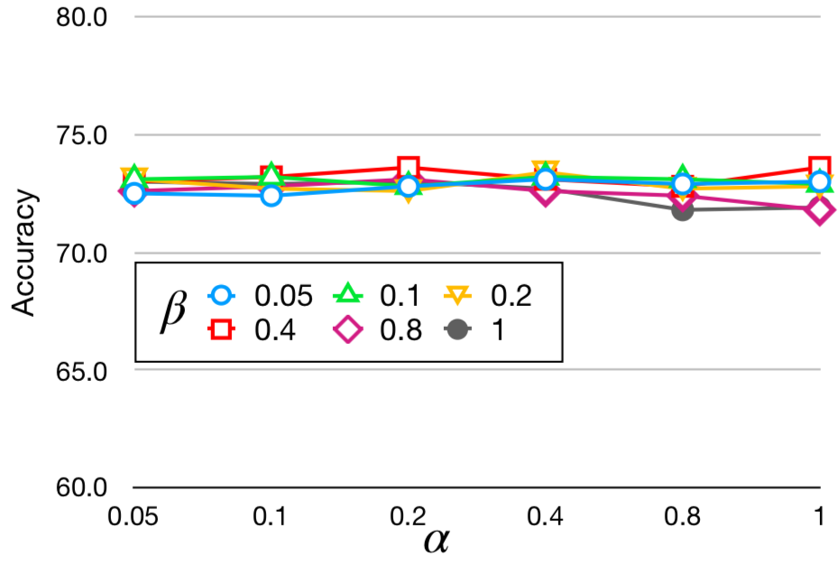 Figure 4
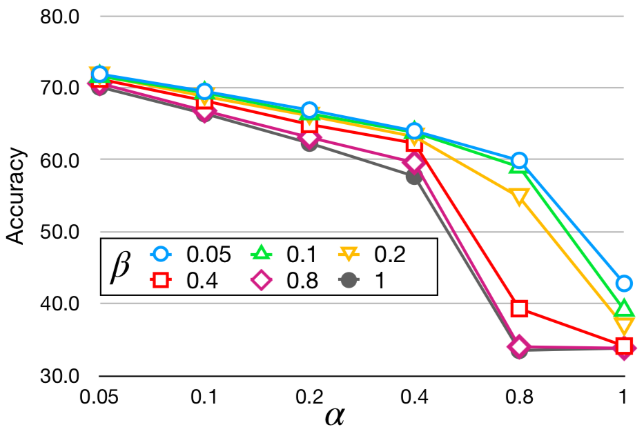 Figure 5
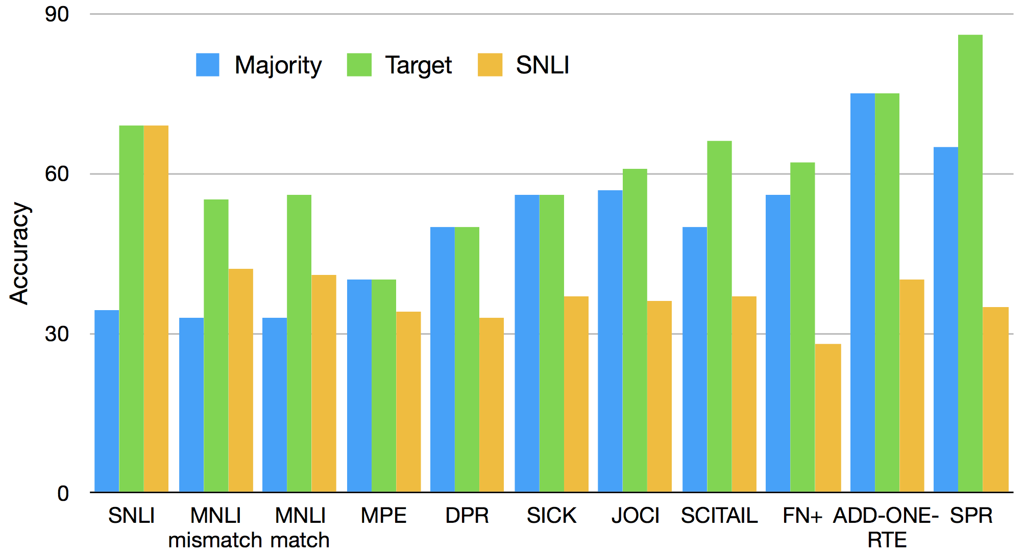 Figure 6
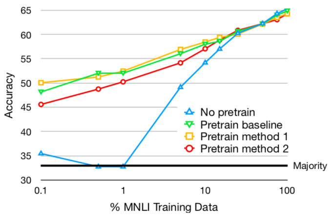 Figure 7
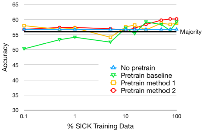 Figure 8
| 0.1 | 0.25 | 0.5 | 1 | 2.5 | 5 | |
|---|---|---|---|---|---|---|
| 0.1 | 50 | 50 | 50 | 50 | 50 | 50 |
| 0.5 | 50 | 50 | 50 | 50 | 50 | 50 |
| 1 | 50 | 50 | 50 | 50 | 50 | 50 |
| 1.5 | 50 | 50 | 50 | 50 | 50 | 100 |
| 2 | 50 | 50 | 50 | 50 | 100 | 100 |
| 2.5 | 50 | 50 | 100 | 75 | 100 | 100 |
| 3 | 50 | 100 | 100 | 100 | 100 | 100 |
| 3.5 | 100 | 100 | 100 | 100 | 100 | 100 |
| 4 | 100 | 100 | 100 | 100 | 100 | 100 |
| 5 | 100 | 100 | 100 | 100 | 100 | 100 |
| 10 | 100 | 100 | 100 | 100 | 100 | 100 |
| 20 | 100 | 100 | 100 | 100 | 100 | 100 |
| 0.1 | 0.25 | 0.5 | 0.75 | 1 | |
|---|---|---|---|---|---|
| 0.1 | 50 | 50 | 50 | 50 | 50 |
| 0.5 | 50 | 50 | 50 | 50 | 50 |
| 1 | 50 | 50 | 50 | 50 | 50 |
| 1.5 | 50 | 50 | 50 | 50 | 50 |
| 2 | 50 | 50 | 50 | 50 | 50 |
| 2.5 | 50 | 50 | 50 | 50 | 50 |
| 3 | 50 | 50 | 100 | 50 | 50 |
| 3.5 | 50 | 50 | 100 | 50 | 50 |
| 4 | 50 | 100 | 100 | 50 | 50 |
| 5 | 50 | 50 | 100 | 100 | 50∗ |
| 10 | 75 | 100 | 100 | 100 | 50∗ |
| 20 | 100 | 100 | 100 | 50∗ | 50∗ |
| Test On Target Dataset | Test On SNLI | ||||||||||||||||
| Target Test Dataset | Baseline | Method 1 | Method 2 | Method 1 | Method 2 | ||||||||||||
| SCITAIL | 58.14 | -0.47 | — | -7.06 | — | -0.18 | — | -9.06 | — | ||||||||
| ADD-ONE-RTE | 66.15 | 0.00 | — | 17.31 | — | -2.29 | — | -49.63 | — | ||||||||
| JOCI | 41.50 | 0.24 | — | -1.87 | — | -0.44 | — | -5.92 | — | ||||||||
| MPE | 57.65 | 0.45 | — | -5.30 | — | -0.57 | — | -0.54 | — | ||||||||
| DPR | 49.86 | 1.10 | — | -0.45 | — | -0.73 | — | -7.81 | — | ||||||||
| MNLI matched | 45.86 | 1.38 | — | -2.10 | — | -1.25 | — | -8.93 | — | ||||||||
| FN+ | 50.87 | 1.61 | — | 6.16 | — | -1.94 | — | -0.44 | — | ||||||||
| MNLI mismatched | 47.57 | 1.67 | — | -3.91 | — | -1.25 | — | -8.93 | — | ||||||||
| SICK | 25.64 | 1.80 | — | 31.11 | — | -0.57 | — | -8.93 | — | ||||||||
| GLUE | 38.50 | 1.99 | — | 4.71 | — | -1.25 | — | -8.93 | — | ||||||||
| SPR | 52.48 | 6.51 | — | 12.94 | — | -1.76 | — | -14.01 | — | ||||||||
| SNLI-hard | 68.02 | -1.75 | — | -12.42 | — | ||||||||||||
| Dataset | Base | Method 1 | |||
|---|---|---|---|---|---|
| JOCI | 41.50 | 39.29 | -2.21 | — | |
| SNLI | 84.22 | 82.40 | -1.82 | — | |
| DPR | 49.86 | 49.41 | -0.45 | — | |
| MNLI matched | 45.86 | 46.12 | 0.26 | — | |
| MNLI mismatched | 47.57 | 48.19 | 0.62 | — | |
| MPE | 57.65 | 58.60 | 0.95 | — | |
| SCITAIL | 58.14 | 60.82 | 2.68 | — | |
| ADD-ONE-RTE | 66.15 | 68.99 | 2.84 | — | |
| GLUE | 38.50 | 41.58 | 3.08 | — | |
| FN+ | 50.87 | 56.31 | 5.44 | — | |
| SPR | 52.48 | 58.68 | 6.20 | — | |
| SICK | 25.64 | 36.59 | 10.95 | — | |
| SNLI-hard | 68.02 | 63.81 | -4.21 | — | |
Peer Reviews
No public reviews on file for this paper yet. If you reviewed it on a platform where reviews are public (OpenReview, ICLR, NeurIPS, ICML), you can paste yours below so the community can read it here.
Code & Models
Videos
No videos yet. Explain this paper in a talk, walkthrough, or lecture? Add one.
Don’t Take the Premise for Granted:
Mitigating Artifacts in Natural Language Inference
Yonatan Belinkov13 Adam Poliak2∗
** Stuart M. Shieber1 Benjamin Van Durme2 Alexander M. Rush1
1**Harvard University 2Johns Hopkins University 3Massachusetts Institute of Technology
{belinkov,shieber,srush}@seas.harvard.edu
{azpoliak,vandurme}@cs.jhu.edu ∗ Equal contribution
Abstract
Natural Language Inference (NLI) datasets often contain hypothesis-only biases—artifacts that allow models to achieve non-trivial performance without learning whether a premise entails a hypothesis. We propose two probabilistic methods to build models that are more robust to such biases and better transfer across datasets. In contrast to standard approaches to NLI, our methods predict the probability of a premise given a hypothesis and NLI label, discouraging models from ignoring the premise. We evaluate our methods on synthetic and existing NLI datasets by training on datasets containing biases and testing on datasets containing no (or different) hypothesis-only biases. Our results indicate that these methods can make NLI models more robust to dataset-specific artifacts, transferring better than a baseline architecture in out of NLI datasets. Additionally, we provide an extensive analysis of the interplay of our methods with known biases in NLI datasets, as well as the effects of encouraging models to ignore biases and fine-tuning on target datasets. 111Our code is available at https://github.com/azpoliak/robust-nli.
1 Introduction
Natural Language Inference (NLI) is often used to gauge a model’s ability to understand a relationship between two texts (Cooper et al., 1996; Dagan et al., 2006). In NLI, a model is tasked with determining whether a hypothesis (a woman is sleeping) would likely be inferred from a premise (a woman is talking on the phone).222This hypothesis contradicts the premise and would likely not be inferred. The development of new large-scale datasets has led to a flurry of various neural network architectures for solving NLI. However, recent work has found that many NLI datasets contain biases, or annotation artifacts, i.e., features present in hypotheses that enable models to perform surprisingly well using only the hypothesis, without learning the relationship between two texts (Gururangan et al., 2018; Poliak et al., 2018b; Tsuchiya, 2018).333We use artifacts and biases interchangeably. For instance, in some datasets, negation words like “not” and “nobody” are often associated with a relationship of contradiction. As a ramification of such biases, models may not generalize well to other datasets that contain different or no such biases.
Recent studies have tried to create new NLI datasets that do not contain such artifacts, but many approaches to dealing with this issue remain unsatisfactory: constructing new datasets (Sharma et al., 2018) is costly and may still result in other artifacts; filtering “easy” examples and defining a harder subset is useful for evaluation purposes (Gururangan et al., 2018), but difficult to do on a large scale that enables training; and compiling adversarial examples (Glockner et al., 2018) is informative but again limited by scale or diversity. Instead, our goal is to develop methods that overcome these biases as datasets may still contain undesired artifacts despite annotation efforts.
Typical NLI models learn to predict an entailment label discriminatively given a premise-hypothesis pair (Figure 1(a)), enabling them to learn hypothesis-only biases. Instead, we predict the premise given the hypothesis and the entailment label, which by design cannot be solved using data artifacts. While this objective is intractable, it motivates two approximate training methods for standard NLI classifiers that are more resistant to biases. Our first method uses a hypothesis-only classifier (Figure 1(b)) and the second uses negative sampling by swapping premises between premise-hypothesis pairs (Figure 1(c)).
We evaluate the ability of our methods to generalize better in synthetic and naturalistic settings. First, using a controlled, synthetic dataset, we demonstrate that, unlike the baseline, our methods enable a model to ignore the artifacts and learn to correctly identify the desired relationship between the two texts. Second, we train models on an NLI dataset that is known to be biased and evaluate on other datasets that may have different or no biases. We observe improved results compared to a fully discriminative baseline in out of target datasets, indicating that our methods generate models that are more robust to annotation artifacts.
An extensive analysis reveals that our methods are most effective when the target datasets have different biases from the source dataset or no noticeable biases. We also observe that the more we encourage the model to ignore biases, the better it transfers, but this comes at the expense of performance on the source dataset. Finally, we show that our methods can better exploit small amounts of training data in a target dataset, especially when it has different biases from the source data.
In this paper, we focus on the transferability of our methods from biased datasets to ones having different or no biases. Elsewhere Belinkov et al. (2019), we have analyzed the effect of these methods on the learned language representations, suggesting that they may indeed be less biased. However, we caution that complete removal of biases remains difficult and is dependent on the techniques used. The choice of whether to remove bias also depends on the goal; in an in-domain scenario certain biases may be helpful and should not necessarily be removed.
In summary, in this paper we make the following contributions:
- •
Two novel methods to train NLI models that are more robust to dataset-specific artifacts.
- •
An empirical evaluation of the methods on a synthetic dataset and naturalistic datasets.
- •
An extensive analysis of the effects of our methods on handling bias.
2 Motivation
A training instance for NLI consists of a hypothesis sentence , a premise statement , and an inference label . A probabilistic NLI model aims to learn a parameterized distribution to compute the probability of the label given the two sentences. We consider NLI models with premise and hypothesis encoders, and , which learn representations of and , and a classification layer, , which learns a distribution over . Typically, this is done by maximizing this discriminative likelihood directly, which will act as our baseline (Figure 1(a)).
However, many NLI datasets contain biases that allow models to perform non-trivially well when accessing just the hypotheses Tsuchiya (2018); Gururangan et al. (2018); Poliak et al. (2018b). This allows models to leverage hypothesis-only biases that may be present in a dataset. A model may perform well on a specific dataset, without identifying whether entails . Gururangan et al. (2018) argue that “the bulk” of many models’ “success [is] attribute[d] to the easy examples”. Consequently, this may limit how well a model trained on one dataset would perform on other datasets that may have different artifacts.
Consider an example where and are strings from , and an environment where entails if and only if the first letters are the same, as in synthetic dataset A. In such a setting, a model should be able to learn the correct condition for to entail . 444 This is equivalent to XOR and is learnable by a MLP.
Synthetic dataset A
True False
True False
Imagine now that an artifact is appended to every entailed (synthetic dataset B). A model of with access only to the hypothesis side can fit the data perfectly by detecting the presence or absence of in , ignoring the more general pattern. Therefore, we hypothesize that a model that learns by training on such data would be misled by the bias and would fail to learn the relationship between the premise and the hypothesis. Consequently, the model would not perform well on the unbiased synthetic dataset A.
Synthetic dataset B (with artifact)
True False
True False
Instead of maximizing the discriminative likelihood directly, we consider maximizing the likelihood of generating the premise conditioned on the hypothesis and the label : . This objective cannot be fooled by hypothesis-only features, and it requires taking the premise into account. For example, a model that only looks for in the above example cannot do better than chance on this objective. However, as comes from the space of all sentences, this objective is much more difficult to estimate.
3 Training Methods
Our goal is to maximize on the training data. While we could in theory directly parameterize this distribution, for efficiency and simplicity we instead write it in terms of the standard and introduce a new term to approximate the normalization:
[TABLE]
Throughout we will assume is a fixed constant ( justified by the dataset assumption that, lacking , and are independent and drawn at random). Therefore, to approximately maximize this objective we need to estimate . We propose two methods for doing so.
3.1 Method 1: Hypothesis-only Classifier
Our first approach is to estimate the term directly. In theory, if labels in an NLI dataset depend on both premises and hypothesis (which Poliak et al. (2018b) call “interesting NLI”), this should be a uniform distribution. However, as discussed above, it is often possible to correctly predict based only on the hypothesis. Intuitively, this model can be interpreted as training a classifier to identify the (latent) artifacts in the data.
We define this distribution using a shared representation between our new estimator and . In particular, the two share an embedding of from the hypothesis encoder . The additional parameters are in the final layer , which we call the hypothesis-only classifier. The parameters of this layer are updated to fit whereas the rest of the parameters in are updated based on the gradients of .
Training is illustrated in Figure 1(b). This interplay is controlled by two hyper-parameters. First, the negative term is scaled by a hyper-parameter . Second, the updates of are weighted by . We therefore minimize the following multitask loss functions (shown for a single example):
[TABLE]
We implement these together with a gradient reversal layer (Ganin & Lempitsky, 2015). As illustrated in Figure 1(b), during back-propagation, we first pass gradients through the hypothesis-only classifier and then reverse the gradients going to the hypothesis encoder (potentially scaling them by ). 555This approach may also be seen as adversarial training with respect to the hypothesis, akin to domain-adversarial neural networks Ganin et al. (2016). However, our methods encourage robustness to latent hypothesis biases, without requiring a domain label.
3.2 Method 2: Negative Sampling
As an alternative to the hypothesis-only classifier, our second method attempts to remove annotation artifacts from the representations by sampling alternative premises. Consider instead writing the normalization term above as,
[TABLE]
where the expectation is uniform and the last step is from Jensen’s inequality.666There are more developed and principled approaches in language modeling for approximating this partition function without having to make this assumption. These include importance sampling Bengio & Senecal (2003), noise-contrastive estimation Gutmann & Hyvärinen (2010), and sublinear partition estimation Rastogi & Van Durme (2015). These are more difficult to apply in the setting of sampling full sentences from an unknown set. We hope to explore methods for applying them in future work. As in Method 1, we define a separate which shares the embedding layers from , and . However, as we are attempting to unlearn hypothesis bias, we block the gradients and do not let it update the premise encoder .777A reviewer asked about gradient blocking. Our motivation was that, for a random premise, we do not have reliable information to update its encoder. However, future work can explore different configurations of gradient blocking. The full setting is shown in Figure 1(c).
To approximate the expectation, we use uniform samples (from other training examples) to replace the premise in a (, )-pair, while keeping the label . We also maximize to learn the artifacts in the hypotheses. We use to control the fraction of randomly sampled ’s (so the total number of examples remains the same). As before, we implement this using gradient reversal scaled by .
[TABLE]
Finally, we share the classifier weights between and . In a sense this is counter-intuitive, since is being trained to unlearn bias, while is being trained to learn it. However, if the models are trained separately, they may learn to co-adapt with each other Elazar & Goldberg (2018). If is not trained well, we might be fooled to think that the representation does not contain any biases, while in fact they are still hidden in the representation. For some evidence that this indeed happens when the models are trained separately, see Belinkov et al. (2019).888 A similar situation arises in neural cryptography (Abadi & Andersen, 2016), where an encryptor Alice and a decryptor Bob communicate while an adversary Eve tries to eavesdrop on their communication. Alice and Bob are analogous to the hypothesis embedding and , while Eve is analogous to . In their asymmetric encryption experiments, Abadi & Andersen observed seemingly secret communication, which on closer look the adversary was able to eavesdrop on.
4 Experimental Setup
To evaluate how well our methods can overcome hypothesis-only biases, we test our methods on a synthetic dataset as well as on a wide range of existing NLI datasets. The scenario we aim to address is when training on a source dataset with biases and evaluating on a target dataset with different or no biases. We first describe the data and experimental setup before discussing the results.
Synthetic Data
We create a synthetic dataset based on the motivating example in Section 2, where entails if and only if their first letters are the same. The training and test sets have 1K examples each, uniformly distributed among the possible entailment relations. In the test set (dataset A), each premise or hypothesis is a single symbol: , where entails iff . In the training set (dataset B), a letter is appended to the hypothesis side in the True examples, but not in the False examples. In order to transfer well to the test set, a model that is trained on this training set needs to learn the underlying relationship—that entails if and only if their first letter is identical—rather than relying on the presence of in the hypothesis side.
Common NLI datasets
Moving to existing NLI datasets, we train models on the Stanford Natural Language Inference dataset (SNLI; Bowman et al., 2015), since it is known to contain significant annotation artifacts. We evaluate the robustness of our methods on other, target datasets.
As target datasets, we use the datasets investigated by Poliak et al. (2018b) in their hypothesis-only study, plus two test sets: GLUE’s diagnostic test set, which was carefully constructed to not contain hypothesis-biases (Wang et al., 2018), and SNLI-hard, a subset of the SNLI test set that is thought to have fewer biases (Gururangan et al., 2018). The target datasets include human-judged datasets that used automatic methods to pair premises and hypotheses, and then relied on humans to label the pairs: SCITAIL (Khot et al., 2018), ADD-ONE-RTE (Pavlick & Callison-Burch, 2016), Johns Hopkins Ordinal Commonsense Inference (JOCI; Zhang et al., 2017), Multiple Premise Entailment (MPE; Lai et al., 2017),color=blue!40]Adam: remove MPE and add it to footnotecolor=red!40]Yonatan: I don’t think we should remove MPE; I just think we should footnote about the split strategy vs combinationcolor=blue!40]Adam: but what we did makes 0 sense though - when we split into , the label L rarely holds across all 4 new pairscolor=red!40]Yonatan: I understand, but is it really 0 sense or has some sense? it just feels odd to exclude it all of a sudden. Don’t other people do the same by chance? If you feel strongly about it, I’ll accept your judgement and let’s remove itcolor=blue!40]Adam: No one would do what we did? Hopefully I’ll run the MPE test experiments soon so we can change the numbers. and Sentences Involving Compositional Knowledge (SICK; Marelli et al., 2014). The target datasets also include datasets recast by White et al. (2017) to evaluate different semantic phenomena: FrameNet+ (FN+; Pavlick et al., 2015), Definite Pronoun Resolution (DPR; Rahman & Ng, 2012), and Semantic Proto-Roles (SPR; Reisinger et al., 2015).999Detailed descriptions of these datasets can be found in Poliak et al. (2018b). As many of these datasets have different label spaces than SNLI, we define a mapping (Appendix A.1) from our models’ predictions to each target dataset’s labels. Finally, we also test on the Multi-genre NLI dataset (MNLI; Williams et al., 2018), a successor to SNLI.101010We leave additional NLI datasets, such as the Diverse NLI Collection Poliak et al. (2018a), for future work.
Baseline & Implementation Details
We use InferSent (Conneau et al., 2017) as our baseline model because it has been shown to work well on popular NLI datasets and is representative of many NLI models. We use separate BiLSTM encoders to learn vector representations of and .111111Many NLI models encode and separately (Rocktäschel et al., 2016; Mou et al., 2016; Liu et al., 2016; Cheng et al., 2016; Chen et al., 2017), although some share information between the encoders via attention (Parikh et al., 2016; Duan et al., 2018).
The vector representations are combined following Mou et al. (2016),121212Specifically, representations are concatenated, subtracted, and multiplied element-wise. and passed to an MLP classifier with one hidden layer. Our proposed methods for mitigating biases use the same technique for representing and combining sentences. Additional implementation details are provided in Appendix A.2.
For both methods, we sweep hyper-parameters , over . For each target dataset, we choose the best-performing model on its development set and report results on the test set.131313For MNLI, since the test sets are not available, we tune on the matched dev set and evaluate on the mismatched dev set, or vice versa. For GLUE, we tune on MNLI matched.
5 Results
5.1 Synthetic Experiments
To examine how well our methods work in a controlled setup, we train on the biased dataset (B), but evaluate on the unbiased test set (A). As expected, without a method to remove hypothesis-only biases, the baseline fails to generalize to the test set. Examining its predictions, we found that the baseline model learned to rely on the presence/absence of the bias term , always predicting True/False respectively.
Table 1 shows the results of our two proposed methods. As we increase the hyper-parameters and , our methods initially behave like the baseline, learning the training set but failing on the test set. However, with strong enough hyper-parameters (moving towards the bottom in the tables), they perform perfectly on both the biased training set and the unbiased test set. For Method 1, stronger hyper-parameters work better. Method 2, in particular, breaks down with too many random samples (increasing ), as expected. We also found that Method 1 did not require as strong as Method 2. From the synthetic experiments, it seems that Method 1 learns to ignore the bias and learn the desired relationship between and across many configurations, while Method 2 requires much stronger .
5.2 Results on existing NLI datasets
Table 2 (left block) reports the results of our proposed methods compared to the baseline in application to the NLI datasets. The method using the hypothesis-only classifier to remove hypothesis-only biases from the model (Method 1) outperforms the baseline in out of target datasets (), though most improvements are small. The training method using negative sampling (Method 2) only outperforms the baseline in datasets, of which are cases where the other method also outperformed the baseline. These gains are much larger than those of Method 1.
We also report results of the proposed methods on the SNLI test set (right block). As our results improve on the target datasets, we note that Method 1’s performance on SNLI does not drastically decrease (small ), even when the improvement on the target dataset is large (for example, in SPR). For this method, the performance on SNLI drops by just an average of 1.11 (0.65 STDV). For Method 2, there is a large decrease on SNLI as results drop by an average of 11.19 (12.71 STDV). For these models, when we see large improvement on a target dataset, we often see a large drop on SNLI. For example, on ADD-ONE-RTE, Method 2 outperforms the baseline by roughly 17% but performs almost 50% lower on SNLI. Based on this, as well as the results on the synthetic dataset, Method 2 seems to be much more unstable and highly dependent on the right hyper-parameters.
6 Analysis
Our results demonstrate that our approaches may be robust to many datasets with different types of bias. We next analyze our results and explore modifications to the experimental setup that may improve model transferability across NLI datasets.
6.1 Interplay with known biases
A priori, we expect our methods to provide the most benefit when a target dataset has no hypothesis-only biases or such biases that differ from ones in the training data. Previous work estimated the amount of bias in NLI datasets by comparing the performance of a hypothesis-only classifier with the majority baseline Poliak et al. (2018b). If the classifier outperforms the baseline, the dataset is said to have hypothesis-only biases. We follow a similar idea for estimating how similar the biases in a target dataset are to those in the source dataset. We compare the performance of a hypothesis-only classifier trained on SNLI and evaluated on each target dataset, to a majority baseline of the most frequent class in each target dataset’s training set (Maj). We also compare to a hypothesis-only classifier trained and tested on each target dataset. 141414A reviewer noted that this method may miss similar bias “types” that are achieved through different lexical items. We note that our use of pre-trained word embeddings might mitigate this concern.
Figure 2 shows the results. When the hypothesis-only model trained on SNLI is tested on the target datasets, the model performs below Maj (except for MNLI), indicating that these target datasets contain different biases than those in SNLI. The largest difference is on SPR: a hypothesis-only model trained on SNLI performs over 50% worse than one trained on SPR. Indeed, our methods lead to large improvements on SPR (Table 2), indicating that they are especially helpful when the target dataset contains different biases. On MNLI, this hypothesis-only model performs 10% above Maj, and roughly 20% worse compared to when trained on MNLI, suggesting that MNLI and SNLI have similar biases. This may explain why our methods only slightly outperform the baseline on MNLI (Table 2).
The hypothesis-only model trained on each target dataset did not outperform Maj on DPR, ADD-ONE-RTE, SICK, and MPE, suggesting that these datasets do not have noticeable hypothesis-only biases. Here, as expected, we observe improvements when our methods are tested on these datasets, to varying degrees (from 0.45 on MPE to 31.11 on SICK). We also see improvements on datasets with biases (high performance of training on each dataset compared to the corresponding majority baseline), most noticeably SPR. The only exception seems to be SCITAIL, where we do not improve despite it having different biases than SNLI. However, when we strengthen and (below), Method 1 outperforms the baseline.
Finally, both methods obtain improved results on the GLUE diagnostic set, designed to be bias-free. We do not see improvements on SNLI-hard, indicating it may still have biases – a possibility acknowledged by Gururangan et al. (2018).
6.2 Stronger hyper-parameters
In the synthetic experiment, we found that increasing and improves the models’ ability to generalize to the unbiased dataset. Does the same apply to natural NLI datasets? We expect that strengthening the auxiliary losses ( in our methods) during training will hurt performance on the original data (where biases are useful), but improve on the target data, which may have different or no biases (Figure 2). To test this, we increase the hyper-parameter values during training; we consider the range . 151515 The synthetic setup required very strong hyper-parameters, possibly due to the clear-cut nature of the task. In the natural NLI setting, moderately strong values sufficed.
While there are other ways to strengthen our methods, e.g., increasing the number or size of hidden layers (Elazar & Goldberg, 2018), we are interested in the effect of and as they control how much bias is subtracted from our baseline model.
Table 3 shows the results of Method 1 with stronger hyper-parameters on the existing NLI datasets. As expected, performance on SNLI test sets (SNLI and SNLI-hard in Table 3) decreases more, but many of the other datasets benefit from stronger hyper-parameters (compared with Table 2). We see the largest improvement on SICK, achieving over 10% increase compared to the 1.8% gain in Table 2. As for Method 2, we found large drops in quality even in our basic configurations (Appendix A.3), so we do not increase the hyper-parameters further. This should not be too surprising, adding too many random premises will lead to a model’s degradation.
6.3 Fine-tuning on target datasets
Our main goal is to determine whether our methods help a model perform well across multiple datasets by ignoring dataset-specific artifacts. In turn, we did not update the models’ parameters on other datasets. But, what if we are given different amounts of training data for a new NLI dataset?
To determine if our approach is still helpful, we updated four models on increasing sizes of training data from two target datasets ( MNLI and SICK). All three training approaches— the baseline, Method 1, and Method 2—are used to pre-train a model on SNLI and fine-tune on the target dataset. The fourth model is the baseline trained only on the target dataset. Both MNLI and SICK have the same label spaces as SNLI, allowing us to hold that variable constant. We use SICK because our methods resulted in good gains on it (Table 2). MNLI’s large training set allows us to consider a wide range of training set sizes.161616 We hold out K examples from the training set for dev as gold labels for the MNLI test set are not publicly available. We evaluate on MNLI’s matched dev set to assure consistent domains when fine-tuning.
Figure 3 shows the results on the dev sets. In MNLI, pre-training is very helpful when fine-tuning on a small amount of new training data, although there is little to no gain from pre-training with either of our methods compared to the baseline. This is expected, as we saw relatively small gains with the proposed methods on MNLI, and can be explained by SNLI and MNLI having similar biases. In SICK, pre-training with either of our methods is better in most data regimes, especially with very small amounts of target training data.171717Note that SICK is a small dataset (10K examples), which explains why the model without pre-training does not benefit from more data, barely surpassing the majority baseline.
25% of the
7 Related Work
Biases and artifacts in NLU datasets
Many natural language undersrtanding (NLU) datasets contain annotation artifacts. Early work on NLI, also known as recognizing textual entailment (RTE), found biases that allowed models to perform relatively well by focusing on syntactic clues alone (Snow et al., 2006; Vanderwende & Dolan, 2006). Recent work also found artifacts in new NLI datasets Tsuchiya (2018); Gururangan et al. (2018); Poliak et al. (2018b).
Other NLU datasets also exhibit biases. In ROC Stories (Mostafazadeh et al., 2016), a story cloze dataset, Schwartz et al. (2017b) obtained a high performance by only considering the candidate endings, without even looking at the story context. In this case, stylistic features of the candidate endings alone, such as the length or certain words, were strong indicators of the correct ending (Schwartz et al., 2017a; Cai et al., 2017). A similar phenomenon was observed in reading comprehension, where systems performed non-trivially well by using only the final sentence in the passage or ignoring the passage altogether (Kaushik & Lipton, 2018). Finally, multiple studies found non-trivial performance in visual question answering (VQA) by using only the question, without access to the image, due to question biases (Zhang et al., 2016; Kafle & Kanan, 2016, 2017; Goyal et al., 2017; Agrawal et al., 2017).
Transferability across NLI datasets
It has been known that many NLI models do not transfer across NLI datasets. Chen Zhang’s thesis Zhang (2010) focused on this phenomena as he demonstrated that “techniques developed for textual entailment“ datasets, e.g., RTE-3, do not transfer well to other domains, specifically conversational entailment Zhang & Chai (2009, 2010). Bowman et al. (2015) and Williams et al. (2018) demonstrated (specifically in their respective Tables 7 and 4) how models trained on SNLI and MNLI may not transfer well across other NLI datasets like SICK. Talman & Chatzikyriakidis (2018) recently reported similar findings using many advanced deep-learning models.
Improving model robustness
Neural networks are sensitive to adversarial examples, primarily in machine vision, but also in NLP (Jia & Liang, 2017; Belinkov & Bisk, 2018; Ebrahimi et al., 2018; Heigold et al., 2018; Mudrakarta et al., 2018; Ribeiro et al., 2018; Belinkov & Glass, 2019). A common approach to improving robustness is to include adversarial examples in training (Szegedy et al., 2014; Goodfellow et al., 2015). However, this may not generalize well to new types of examples (Xiaoyong Yuan, 2017; tramèr2018ensemble).
Domain-adversarial neural networks aim to increase robustness to domain change, by learning to be oblivious to the domain using gradient reversals (Ganin et al., 2016). Our methods rely similarly on gradient reversals when encouraging models to ignore dataset-specific artifacts. One distinction is that domain-adversarial networks require knowledge of the domain at training time, while our methods learn to ignore latent artifacts and do not require direct supervision in the form of a domain label.
Others have attempted to remove biases from learned representations, e.g., gender biases in word embeddings (Bolukbasi et al., 2016) or sensitive information like sex and age in text representations (Li et al., 2018). However, removing such attributes from text representations may be difficult (Elazar & Goldberg, 2018). In contrast to this line of work, our final goal is not the removal of such attributes per se; instead, we strive for more robust representations that better transfer to other datasets, similar to Li et al. (2018).
Recent work has applied adversarial learning to NLI. Minervini & Riedel (2018) generate adversarial examples that do not conform to logical rules and regularize models based on those examples. Similarly, Kang et al. (2018) incorporate external linguistic resources and use a GAN-style framework to adversarially train robust NLI models. In contrast, we do not use external resources and we are interested in mitigating hypothesis-only biases. Finally, a similar approach has recently been used to mitigate biases in VQA (Ramakrishnan et al., 2018; Grand & Belinkov, 2019).
8 Conclusion
Biases in annotations are a major source of concern for the quality of NLI datasets and systems. We presented a solution for combating annotation biases by proposing two training methods to predict the probability of a premise given an entailment label and a hypothesis. We demonstrated that this discourages the hypothesis encoder from learning the biases to instead obtain a less biased representation. When empirically evaluating our approaches, we found that in a synthetic setting, as well as on a wide-range of existing NLI datasets, our methods perform better than the traditional training method to predict a label given a premise-hypothesis pair. Furthermore, we performed several analyses into the interplay of our methods with known biases in NLI datasets, the effects of stronger bias removal, and the possibility of fine-tuning on the target datasets.
Our methodology can be extended to handle biases in other tasks where one is concerned with finding relationships between two objects, such as visual question answering, story cloze completion, and reading comprehension. We hope to encourage such investigation in the broader community.
Acknowledgements
We would like to thank Aviad Rubinstein and Cynthia Dwork for discussing an earlier version of this work and the anonymous reviewers for their useful comments. Y.B. was supported by the Harvard Mind, Brain, and Behavior Initiative. A.P. and B.V.D were supported by JHU-HLTCOE and DARPA LORELEI. A.M.R gratefully acknowledges the support of NSF 1845664. Views and conclusions contained in this publication are those of the authors and should not be interpreted as representing official policies or endorsements of DARPA or the U.S. Government.
Appendix A Appendix
A.1 Mapping labels
Each premise-hypothesis pair in SNLI is labeled as entailment, neutral, or contradiction. MNLI, SICK, and MPE use the same label space. Examples in JOCI are labeled on a 5-way ordinal scale. We follow Poliak et al. (2018b) by converting it “into 3-way NLI tags where 1 maps to contradiction, 2-4 maps to neutral, and 5 maps to entailment.” Since examples in SCITAIL are labeled as entailment or neutral, when evaluating on SCITAIL, we convert the model’s contradiction to neutral. ADD-ONE-RTE and the recast datasets also model NLI as a binary prediction task. However, their label sets are entailed and not-entailed. In these cases, when the models predict entailment, we map the label to entailed, and when the models predict neutral or contradiction, we map the label to not-entailed.
A.2 Implementation details
For our experiments on the synthetic dataset, the characters are embedded with 10-dimensional vectors. Input strings are represented as a sum of character embeddings, and the premise-hypothesis pair is represented by a concatenation of these embeddings. The classifiers are single-layer MLPs of size 20 dimensions. We train these models with SGD until convergence. For the traditional NLI datasets, we use pre-computed 300-dimensional GloVe embeddings Pennington et al. (2014) .181818Specifically, glove.840B.300d.zip. The sentence representations learned by the BiLSTM encoders and the MLP classifier’s hidden layer have a dimensionality of 2048 and 512 respectively. We follow InferSent’s training regime, using SGD with an initial learning rate of 0.1 and optional early stopping. See Conneau et al. (2017) for details.
A.3 Hyper-parameter sweeps
Here we provide 10-fold cross-validation results on a subset of the SNLI training data (50K sentences) with different settings of our hyper-parameters. Figure 4(b) shows the dev set results with different configurations of Method 2. Notice that performance degrades quickly when we increase the fraction of random premises (large ). In contrast, the results with Method 1 (Figure 4(a)) are more stable.
The reference list from the paper itself. Each links out to its DOI / PubMed record.
- 1Abadi & Andersen (2016) Martín Abadi and David G. Andersen. Learning to protect communications with adversarial neural cryptography. ar Xiv , 2016. URL https://arxiv.org/abs/1610.06918 .
- 2Agrawal et al. (2017) Aishwarya Agrawal, Dhruv Batra, Devi Parikh, and Aniruddha Kembhavi. Don’t Just Assume; Look and Answer: Overcoming Priors for Visual Question Answering. ar Xiv preprint ar Xiv:1712.00377 , 2017.
- 3Belinkov & Bisk (2018) Yonatan Belinkov and Yonatan Bisk. Synthetic and Natural Noise Both Break Neural Machine Translation. In International Conference on Learning Representations , 2018. URL https://openreview.net/forum?id=BJ 8v Jeb C- .
- 4Belinkov & Glass (2019) Yonatan Belinkov and James Glass. Analysis Methods in Neural Language Processing: A Survey. Transactions of the Association for Computational Linguistics (TACL) , 7:49–72, 2019. doi: 10.1162/tacl“˙a“˙00254 . URL https://doi.org/10.1162/tacl_a_00254 . · doi ↗
- 5Belinkov et al. (2019) Yonatan Belinkov, Adam Poliak, Stuart M. Shieber, Benjamin Van Durme, and Alexander Rush. On Adversarial Removal of Hypothesis-only Bias in Natural Language Inference. In Proceedings of the Eighth Joint Conference on Lexical and Computational Semantics (*SEM, Oral presentation) , June 2019.
- 6Bengio & Senecal (2003) Yoshua Bengio and Jean-Sébastien Senecal. Quick Training of Probabilistic Neural Nets by Importance Sampling. In Proceedings of the Ninth International Workshop on Artificial Intelligence and Statistics, AISTATS 2003, Key West, Florida, USA, January 3-6, 2003 , pp. 1–9, 2003. URL http://research.microsoft.com/en-us/um/cambridge/events/aistats 2003/proceedings/164.pdf .
- 7Bolukbasi et al. (2016) Tolga Bolukbasi, Kai-Wei Chang, James Y Zou, Venkatesh Saligrama, and Adam T Kalai. Man is to computer programmer as woman is to homemaker? debiasing word embeddings. In Advances in Neural Information Processing Systems , pp. 4349–4357, 2016.
- 8Bowman et al. (2015) Samuel R. Bowman, Gabor Angeli, Christopher Potts, and Christopher D. Manning. A large annotated corpus for learning natural language inference. In Proceedings of the 2015 Conference on Empirical Methods in Natural Language Processing (EMNLP) . Association for Computational Linguistics, 2015.