Forced three-wave interactions of capillary-gravity surface waves
Annette Cazaubiel, Florence Haudin, Eric Falcon, Michael Berhanu

TL;DR
This paper experimentally investigates forced three-wave interactions of capillary-gravity waves, revealing how viscous dissipation influences wave coupling and leads to daughter waves that do not follow the linear dispersion relation.
Contribution
It demonstrates experimentally that viscous dissipation causes a forced three-wave interaction mechanism, expanding the understanding of wave coupling beyond traditional resonant conditions.
Findings
Daughter waves can be generated without satisfying the dispersion relation.
Viscous dissipation broadens the transfer function bandwidth.
Forced interactions significantly impact wave turbulence dynamics.
Abstract
{Three-wave resonant interactions constitute an essential nonlinear mechanism coupling capillary surface waves. In a previous work, Haudin et al. [Phys. Rev E 93, 043110 (2016)], we have characterized experimentally the generation by this mechanism of a daughter wave, whose amplitude saturates due to the viscous dissipation. Here, we show experimentally the generation of a daughter wave verifying the resonant conditions, but not the dispersion relation.} By modeling the response of the free surface at the lowest nonlinear order, we explain this observation as a forced interaction. {The bandwidth of the linear transfer function of the free surface is indeed increased by the significant viscous dissipation.} The observation of free surface excitations not following the linear dispersion relation then becomes possible. This forced three-wave interaction mechanism could have important…
Click any figure to enlarge with its caption.
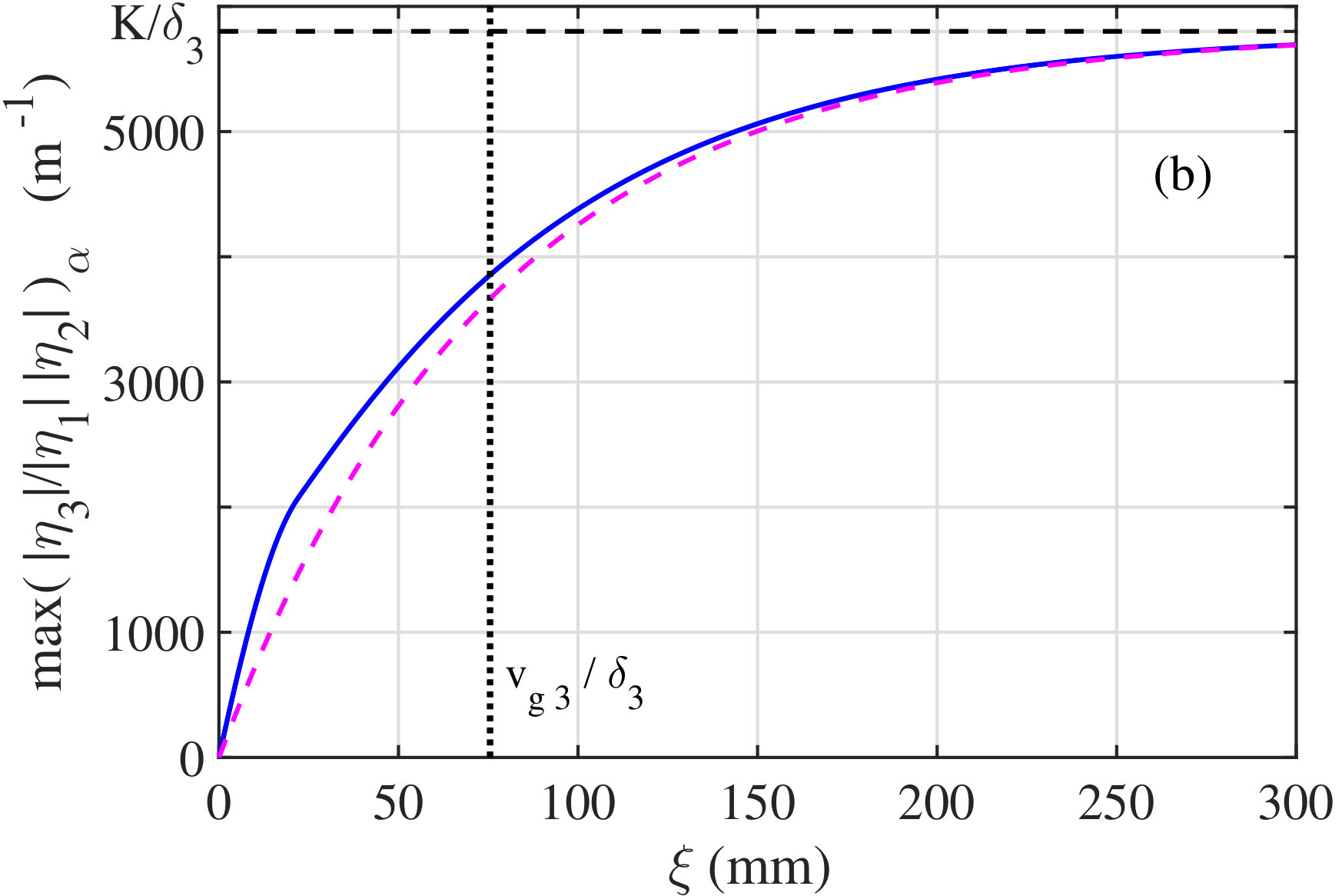 Figure 1
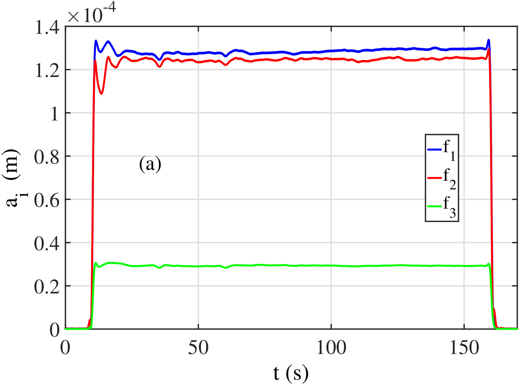 Figure 2
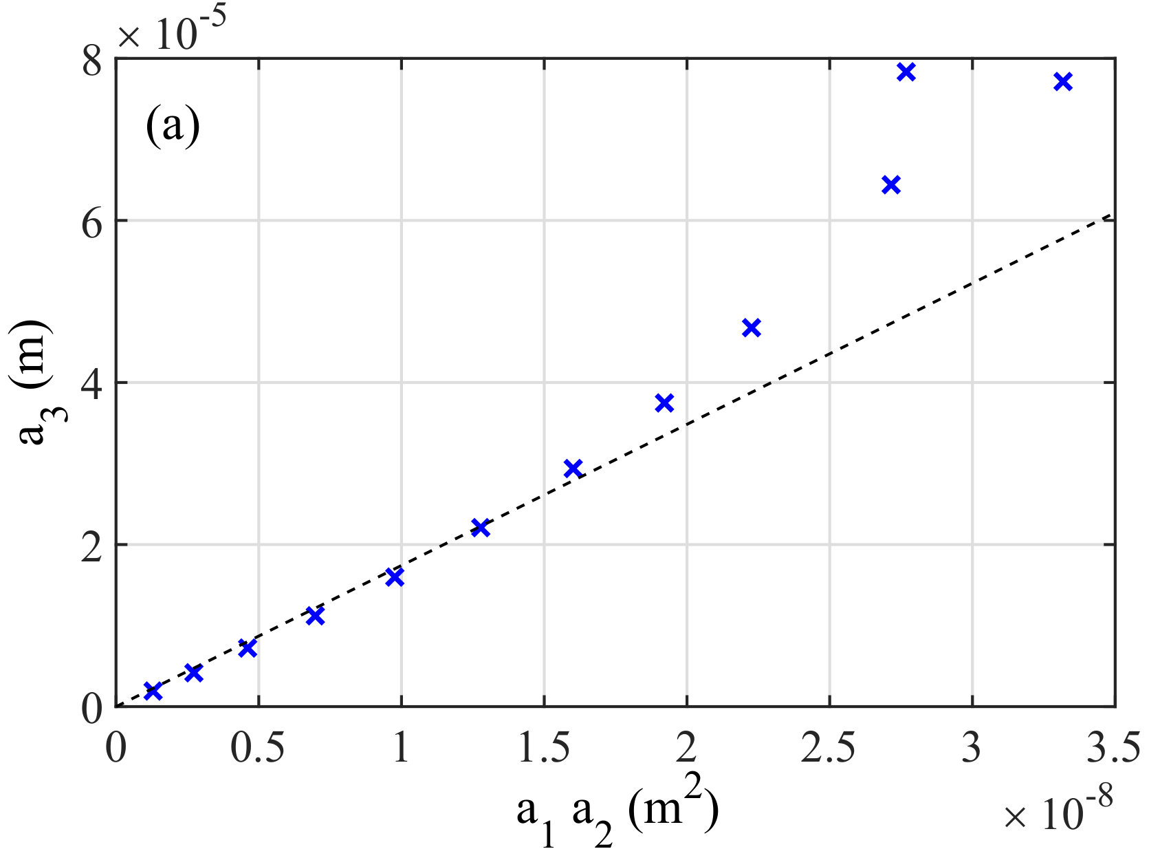 Figure 3
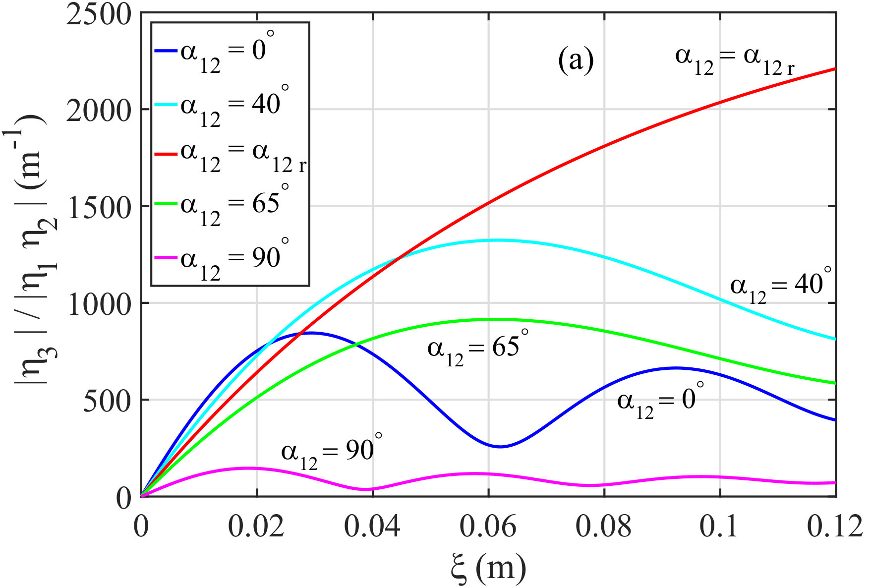 Figure 4
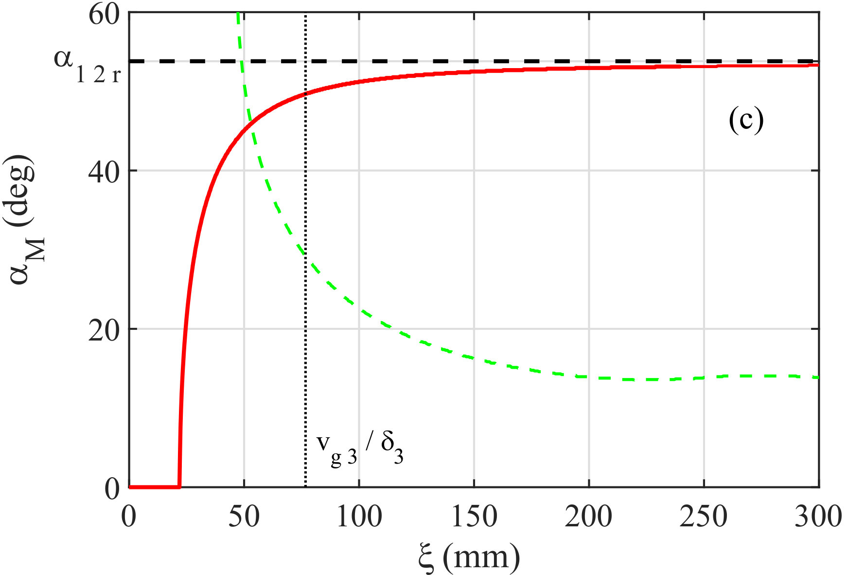 Figure 5
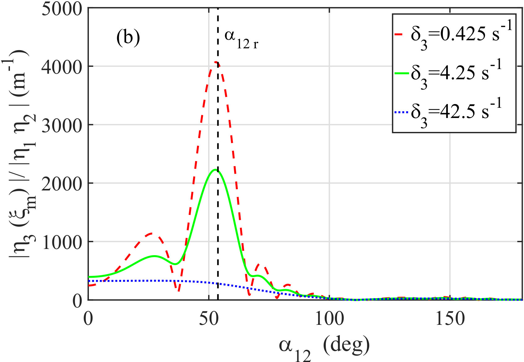 Figure 6
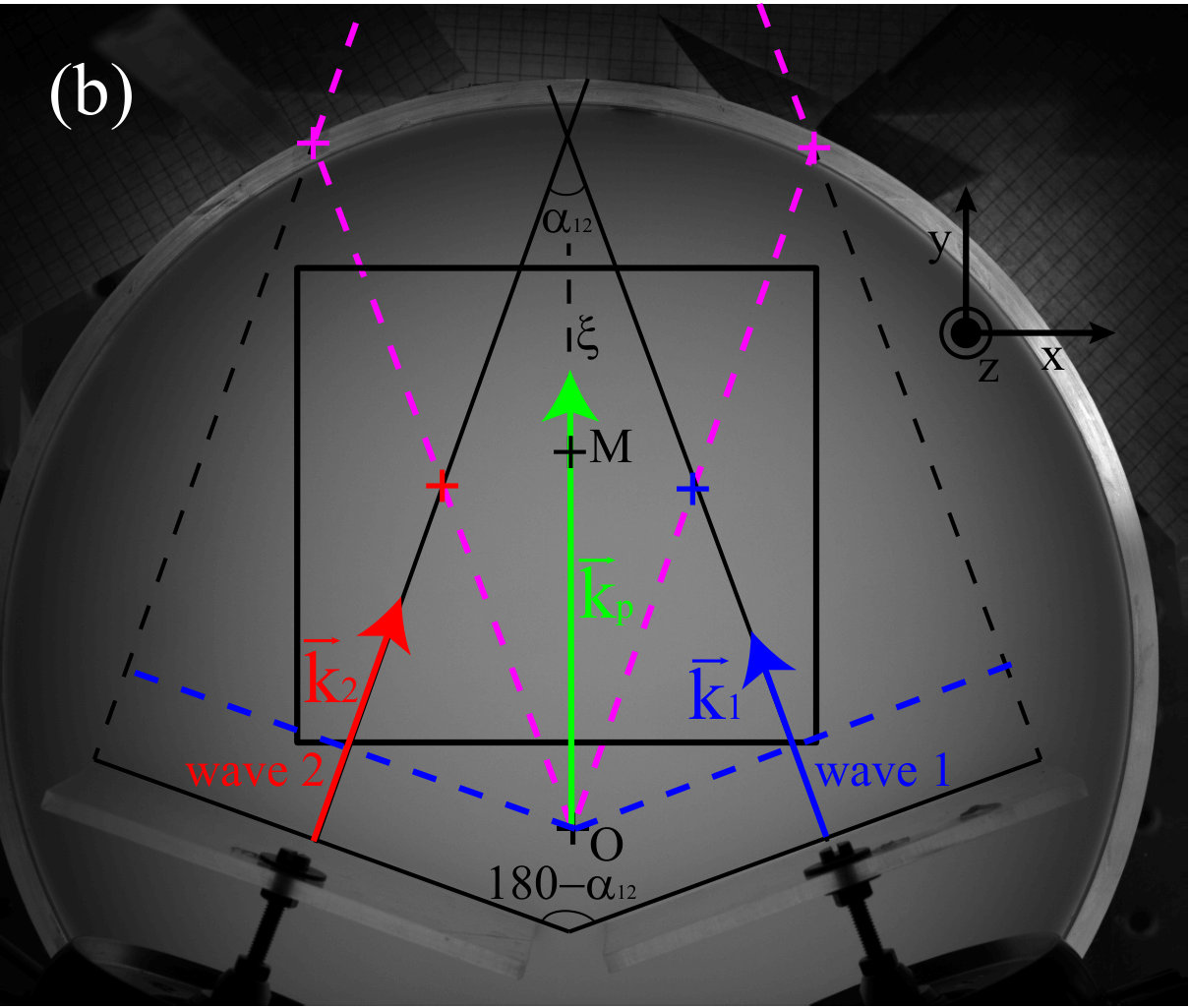 Figure 7
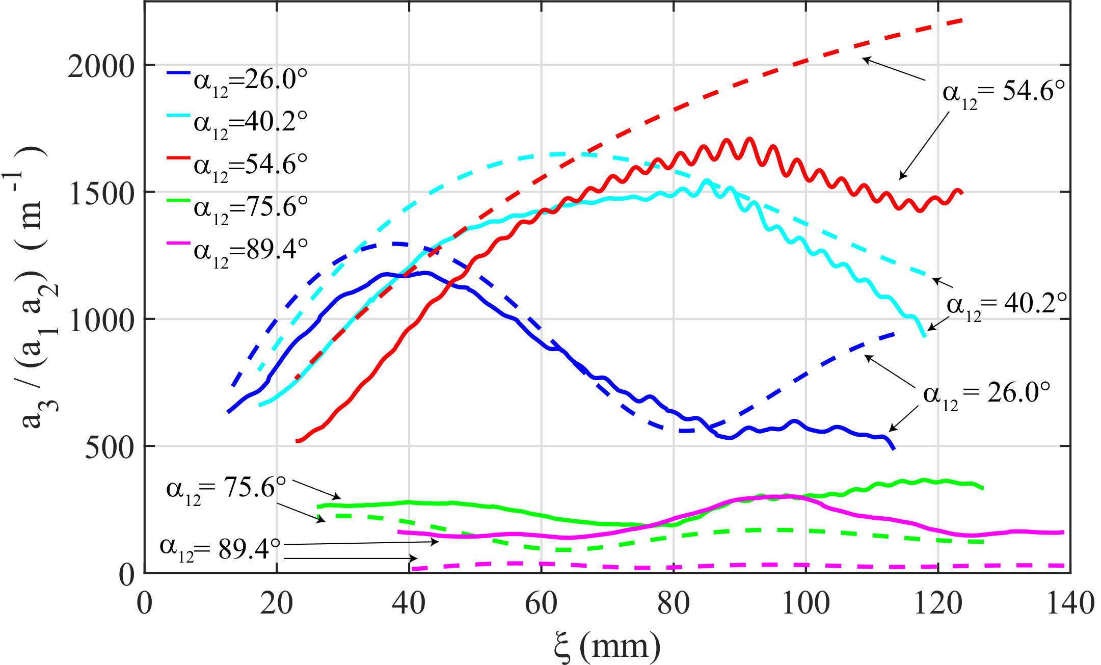 Figure 45
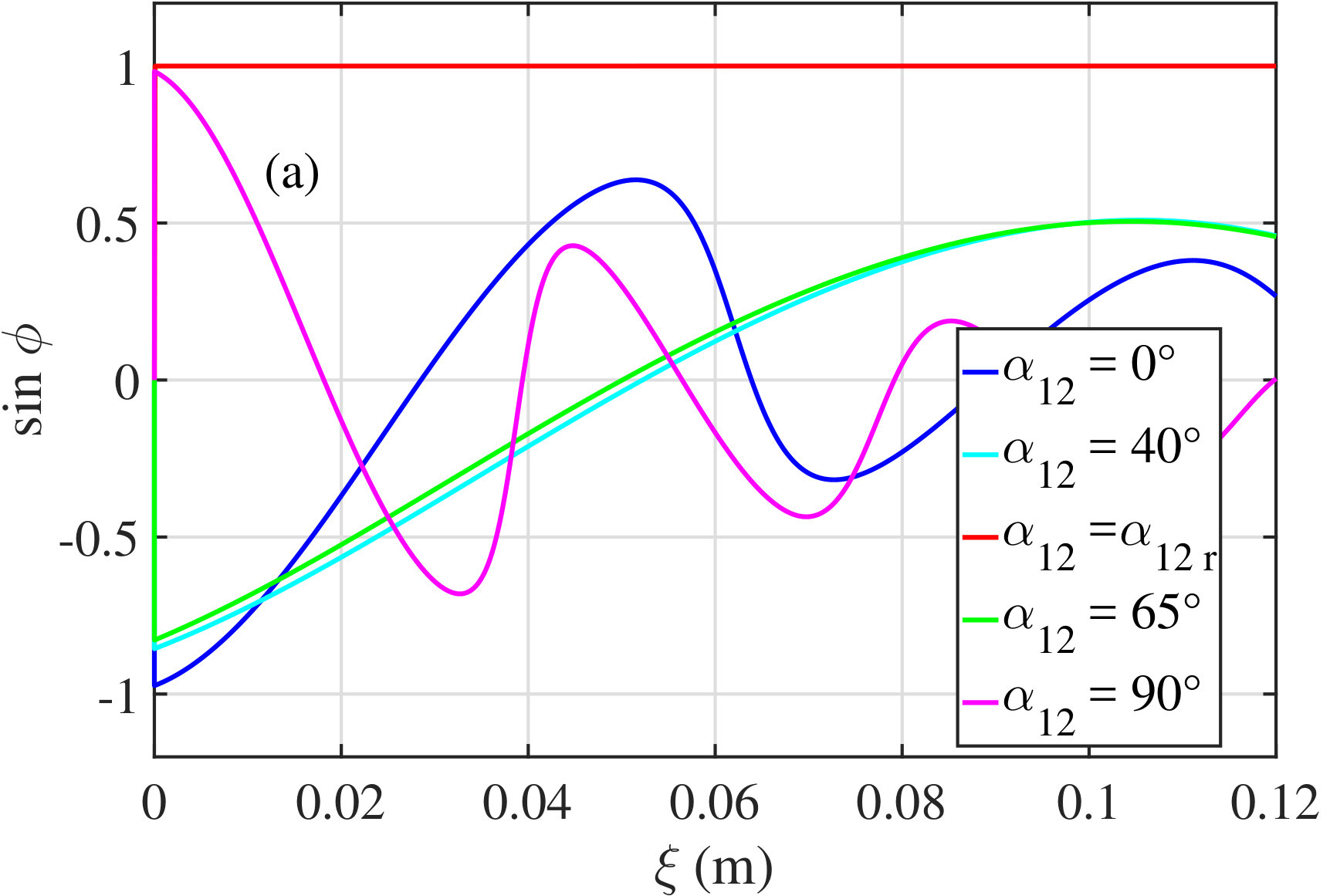 Figure 9
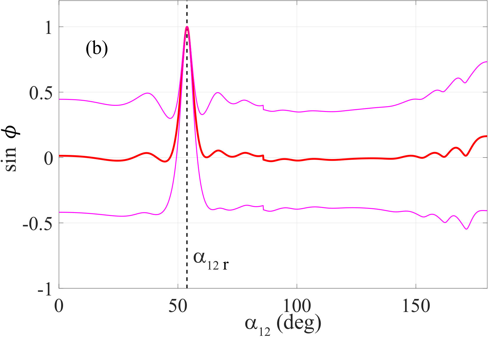 Figure 10
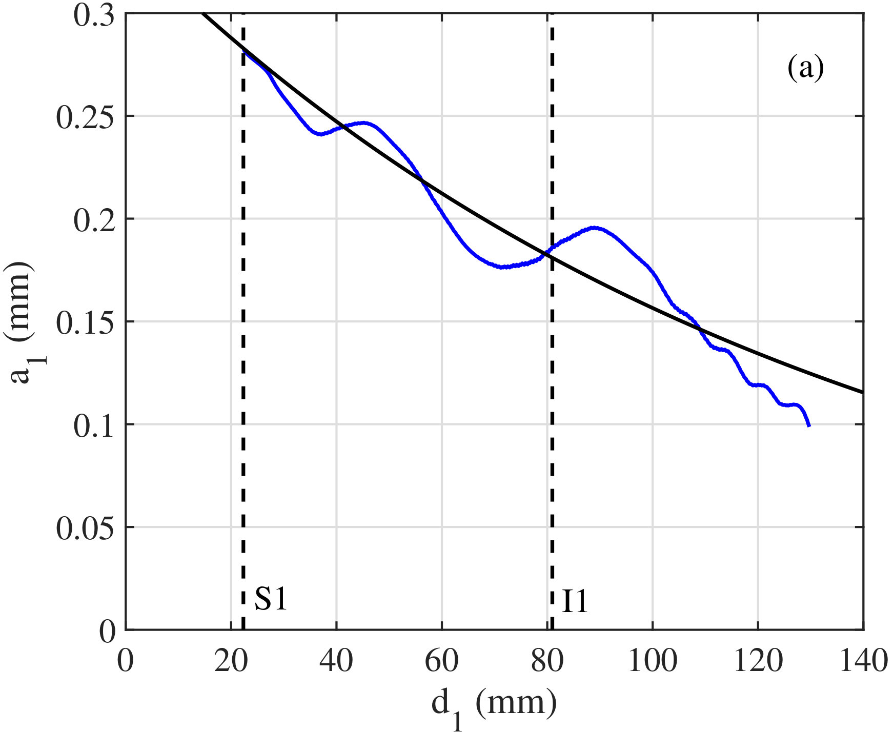 Figure 11
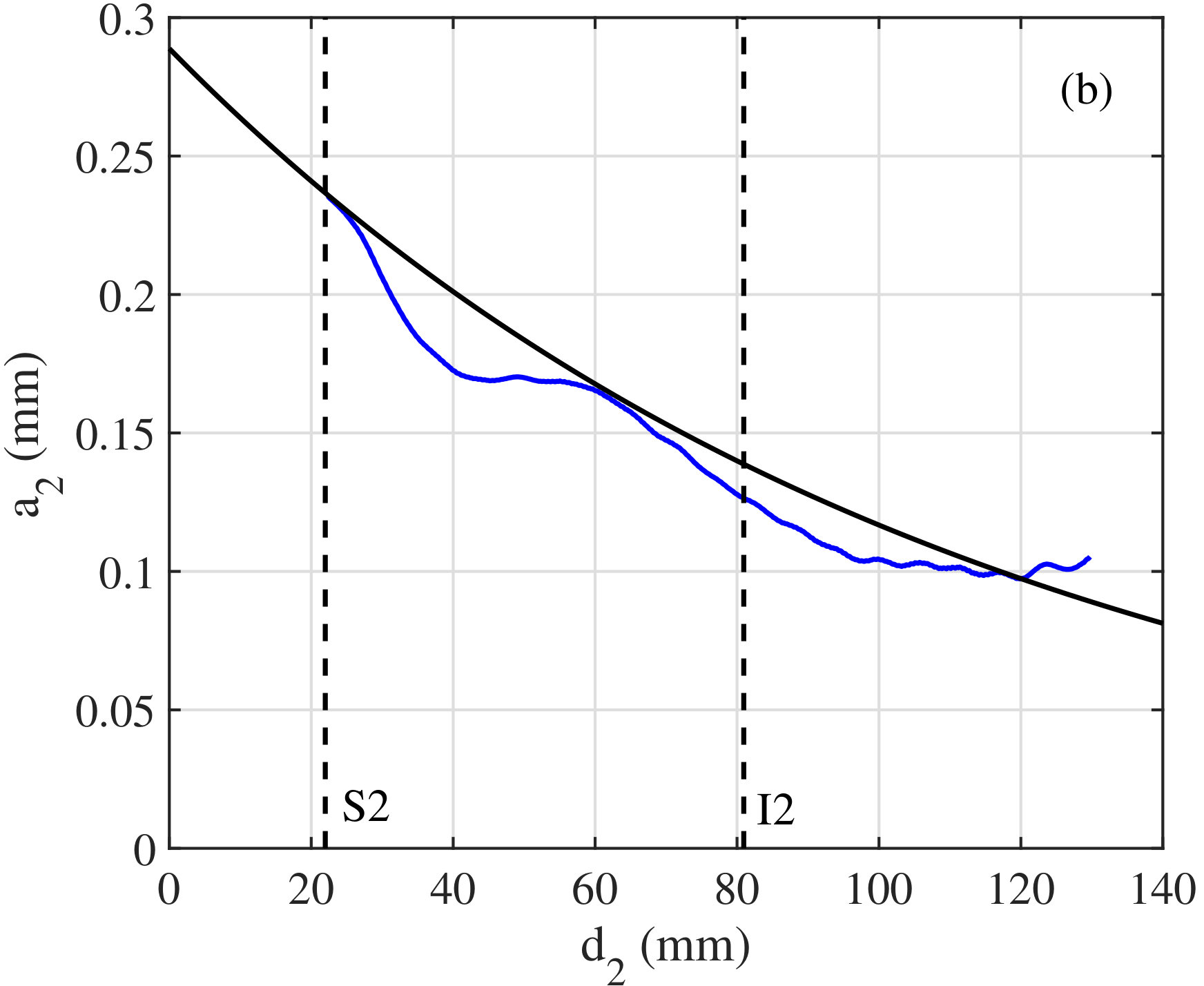 Figure 12
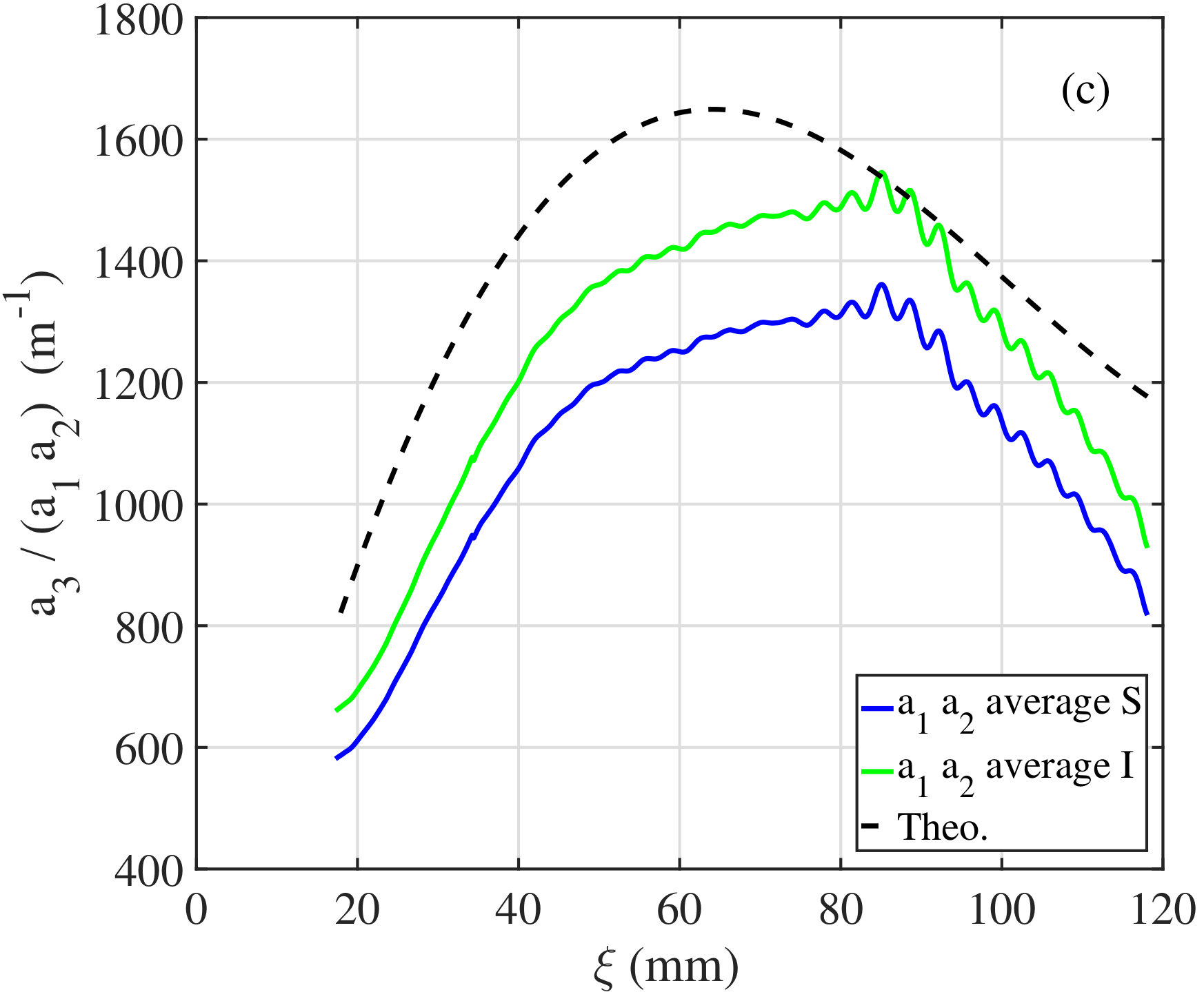 Figure 13
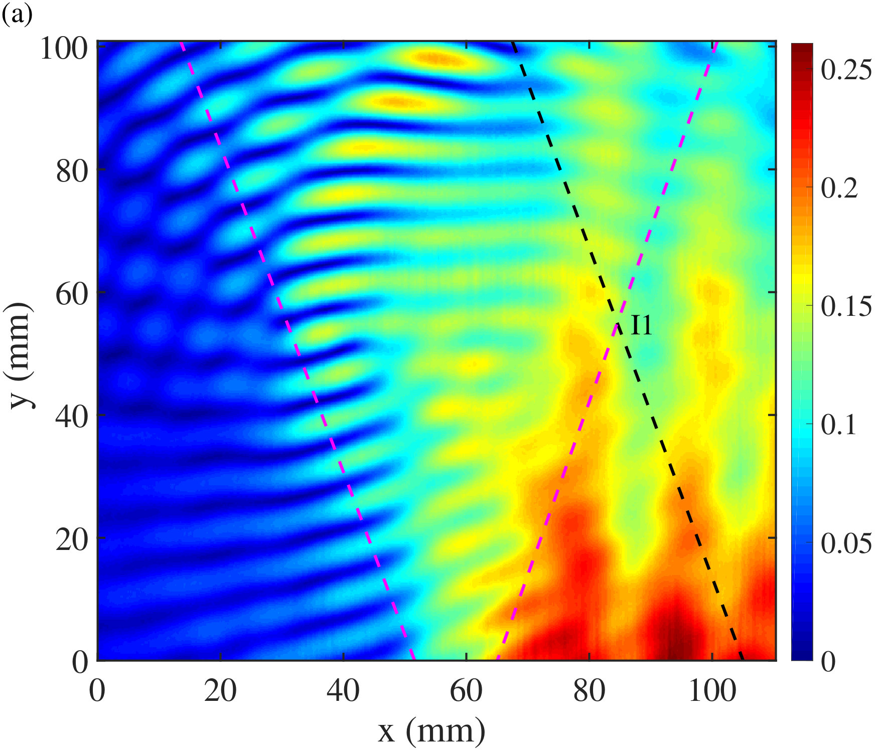 Figure 14
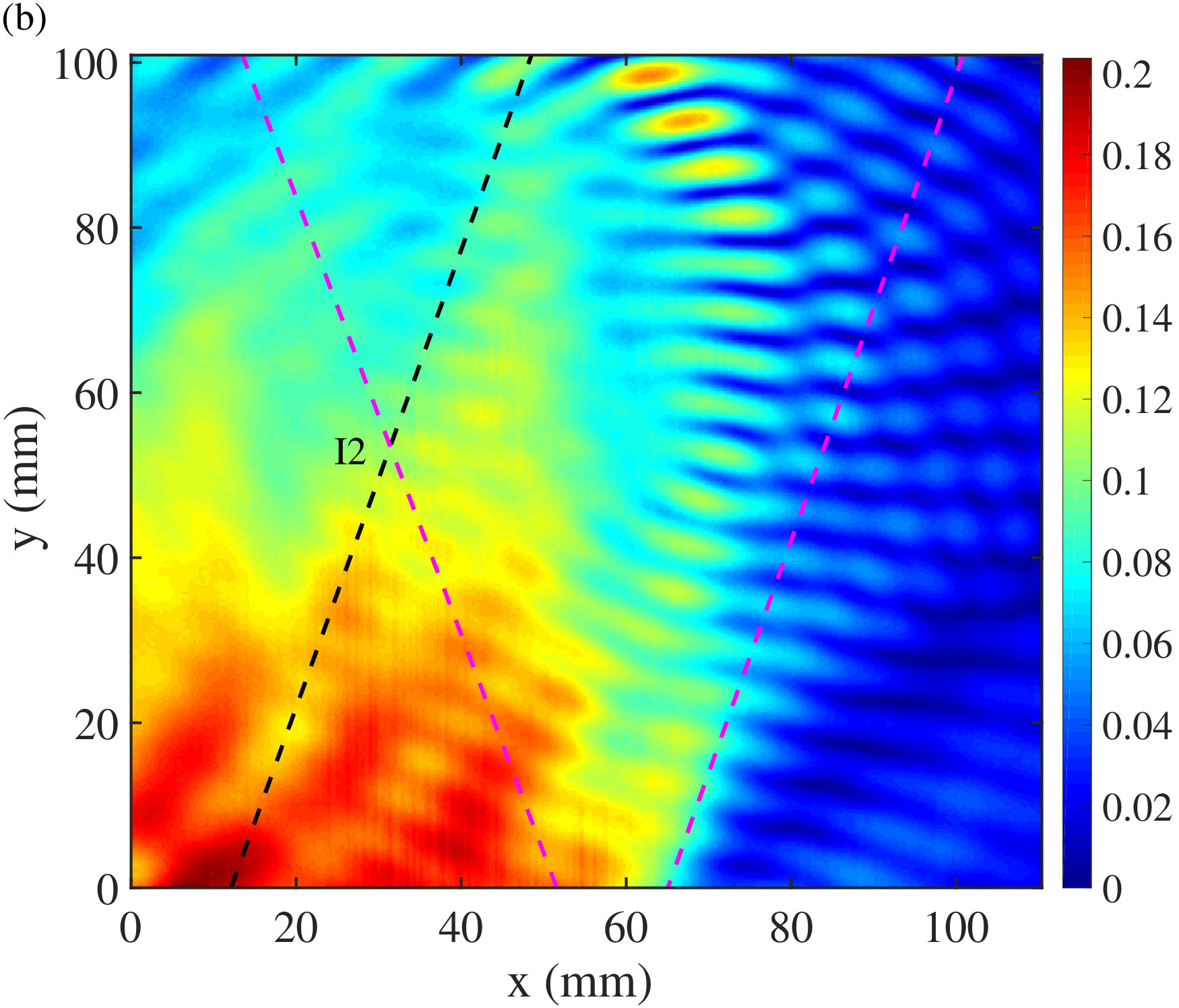 Figure 15
 Figure 16
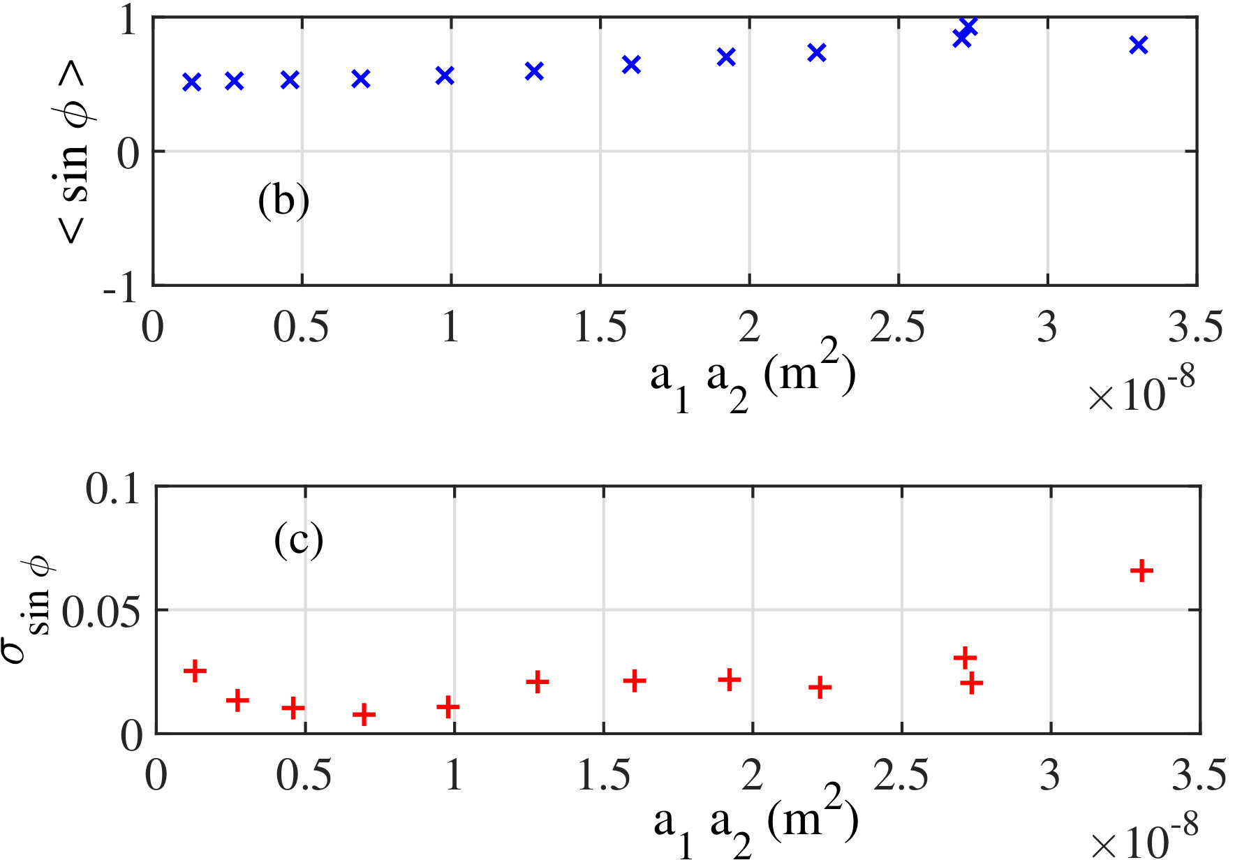 Figure 17
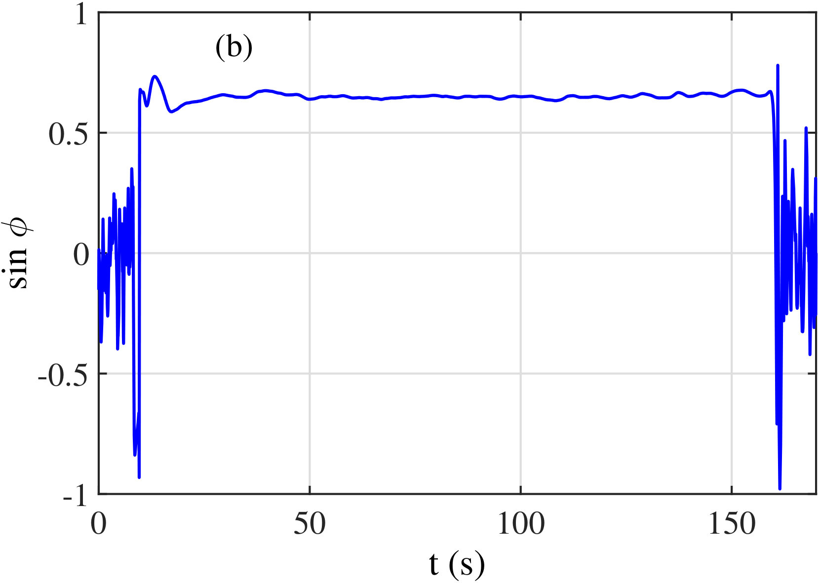 Figure 18
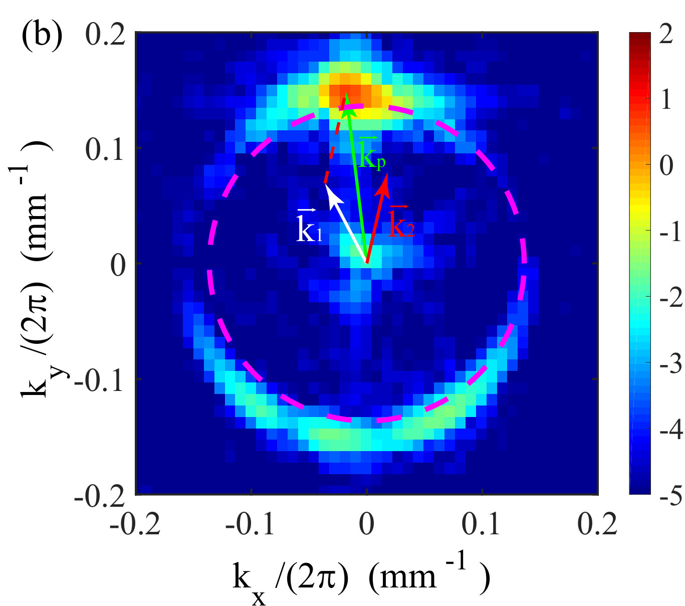 Figure 19
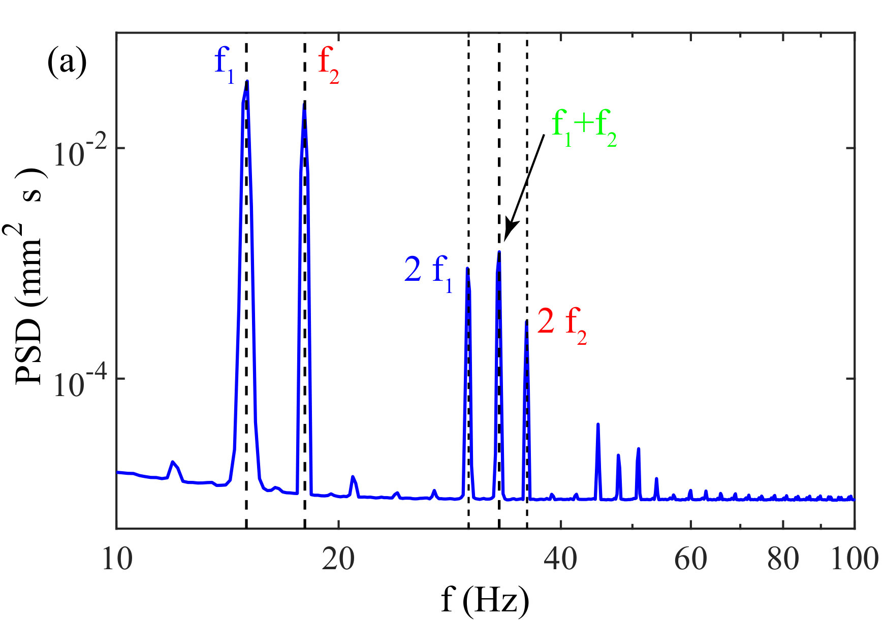 Figure 20
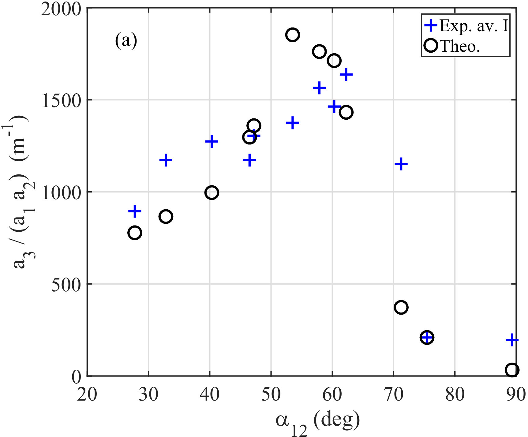 Figure 21
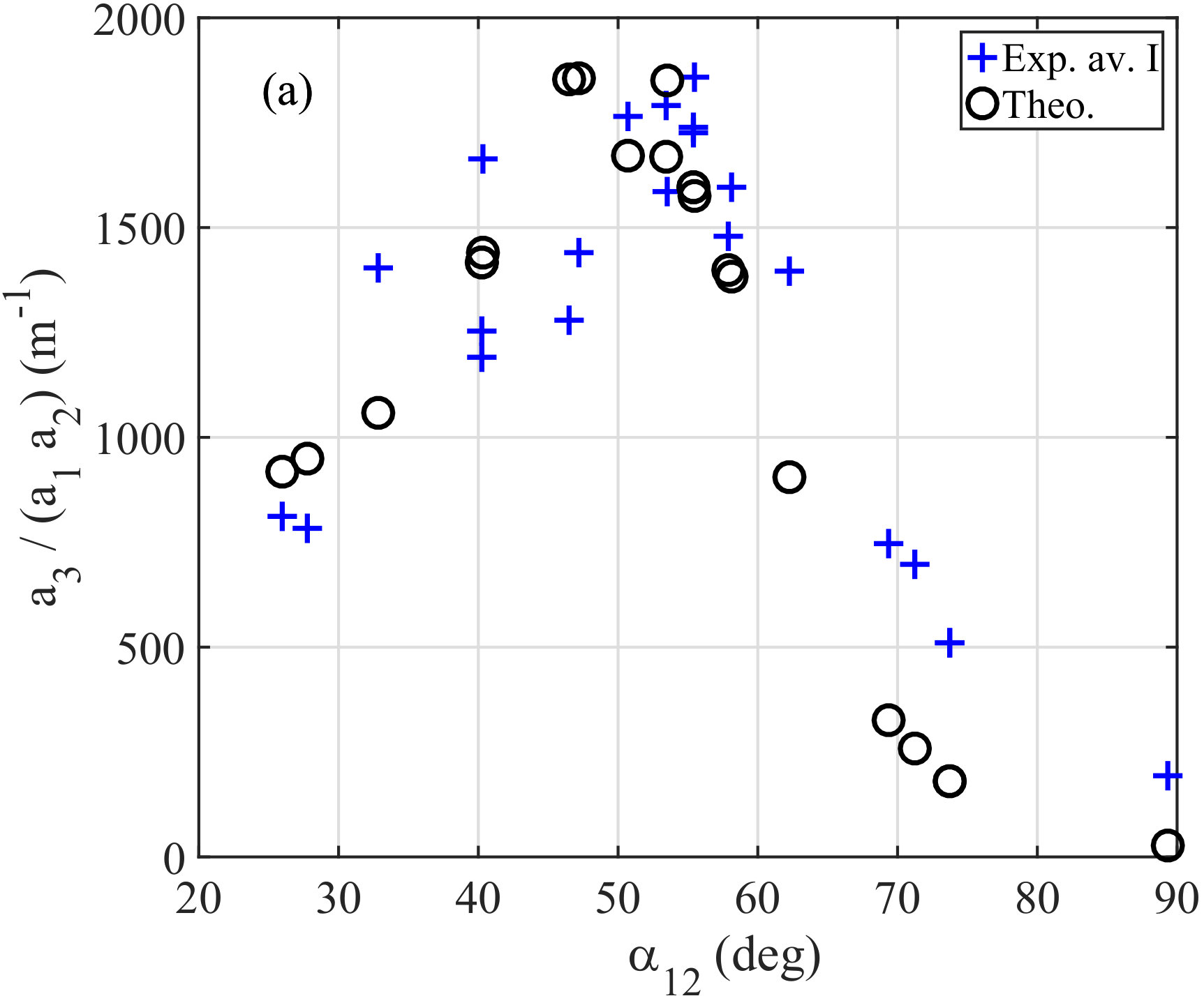 Figure 22
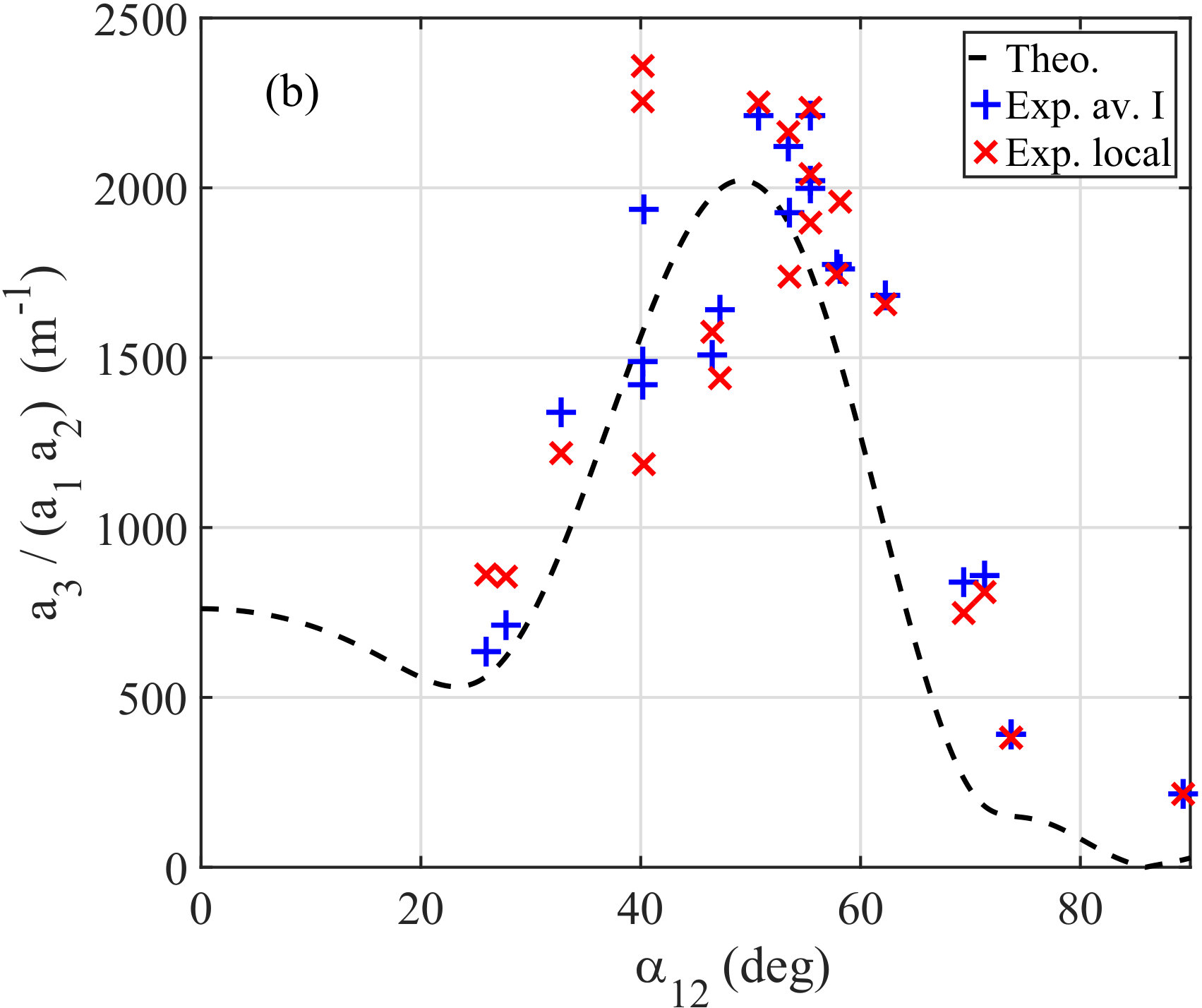 Figure 23
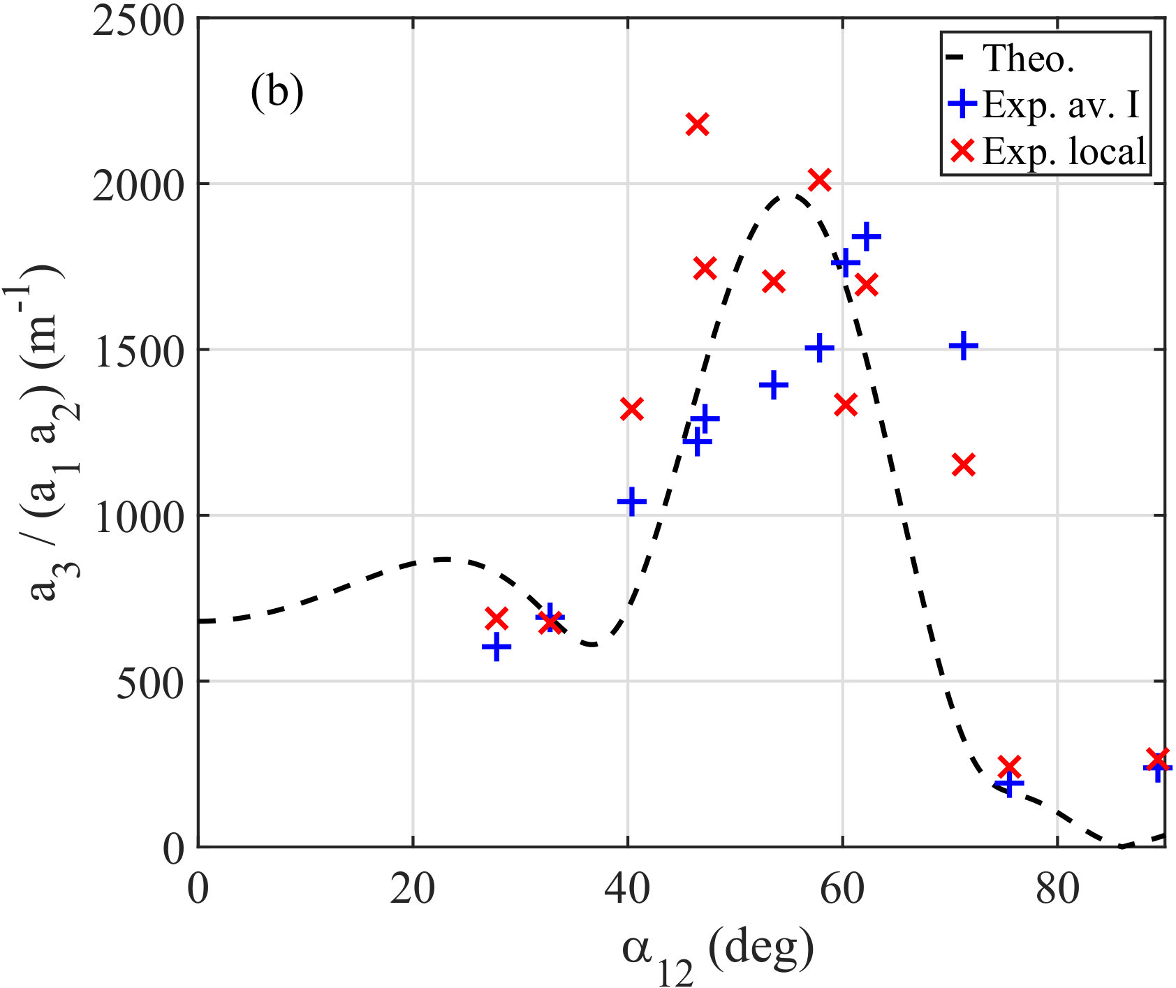 Figure 24
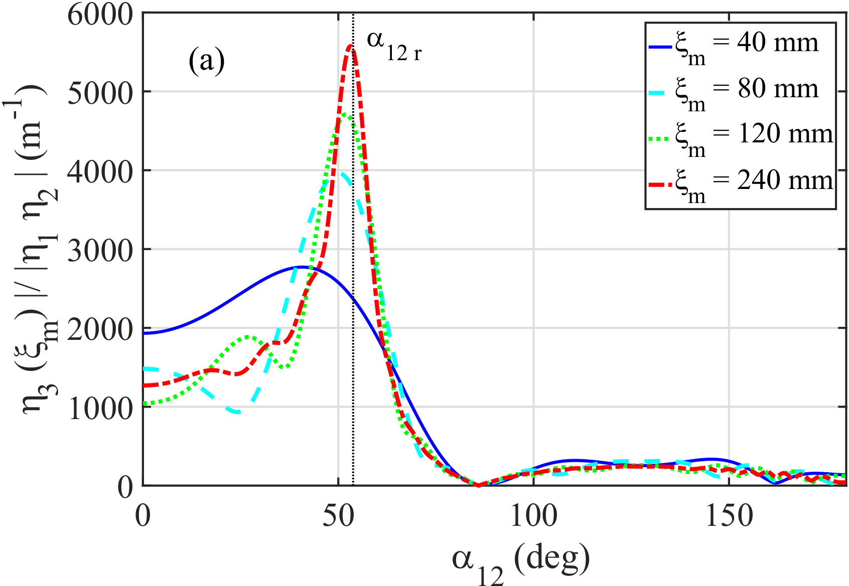 Figure 25
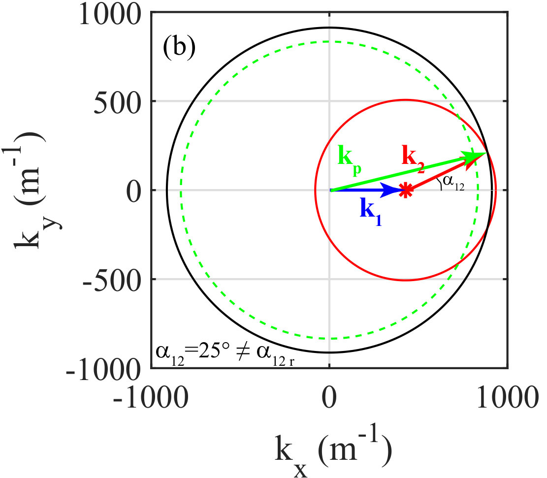 Figure 26
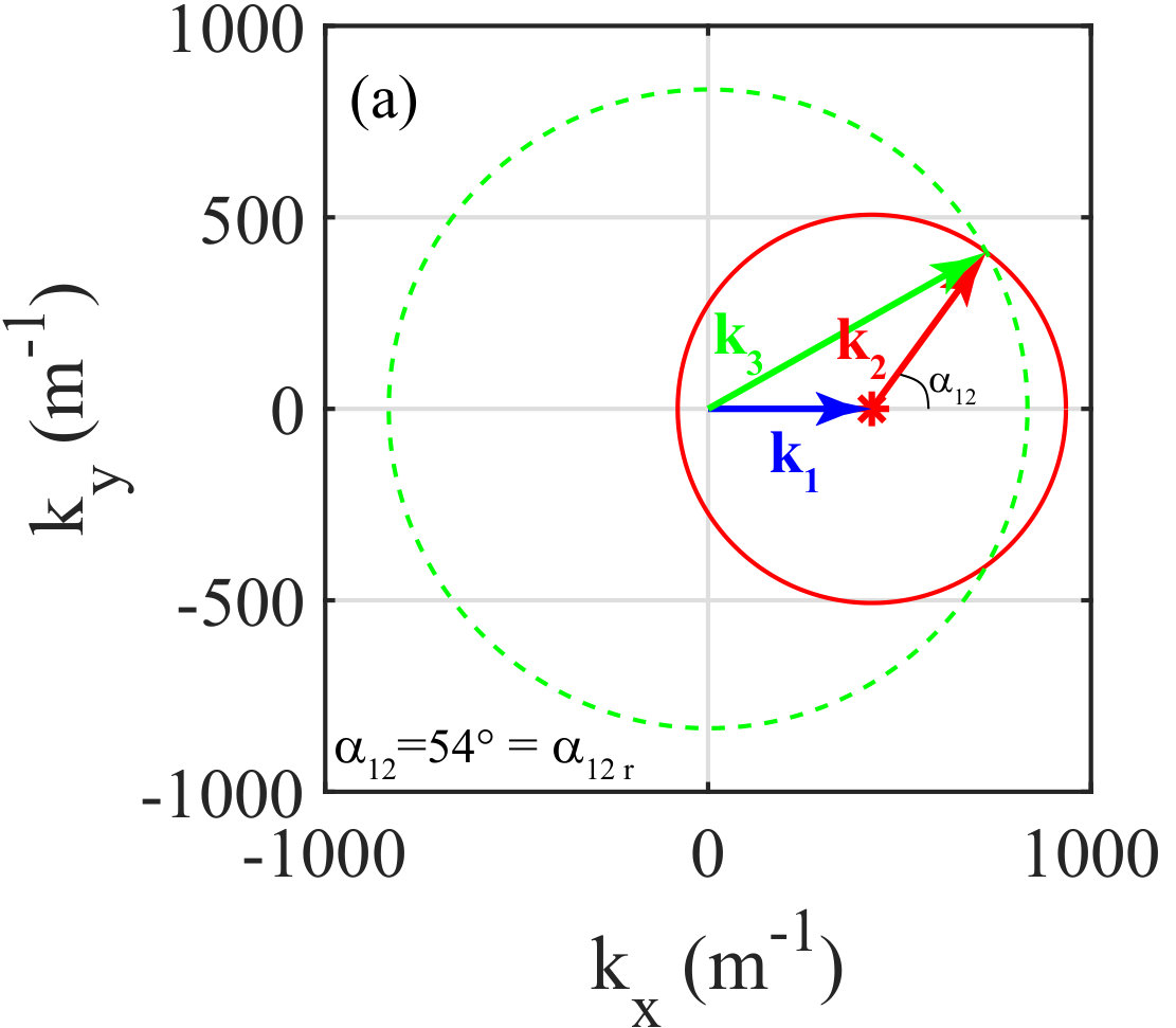 Figure 27
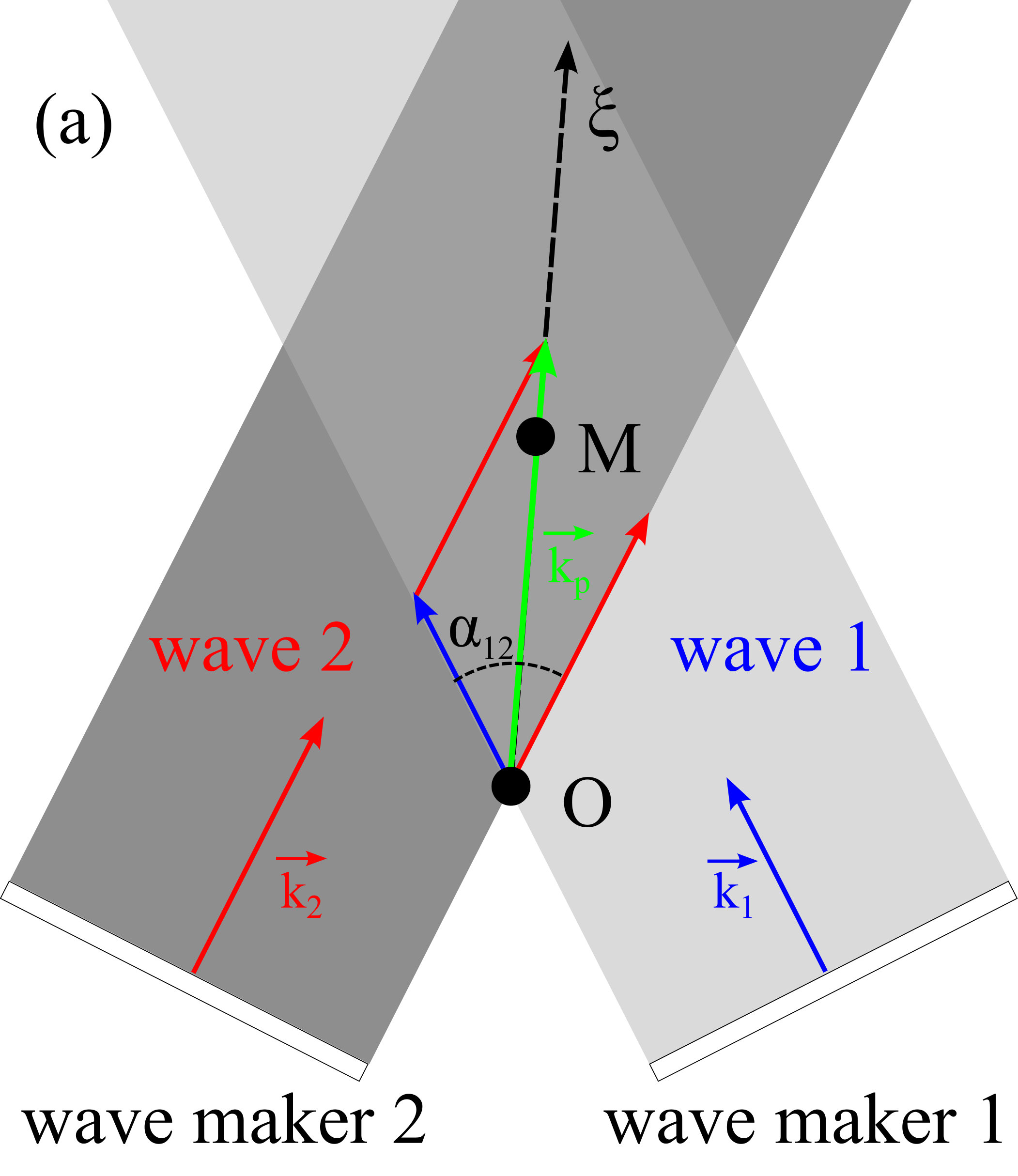 Figure 28
| Frequency of the wave (Hz) | (m | (m s-1) | (m s-1) | (s | |
|---|---|---|---|---|---|
| 428 | - | 0.220 | 0.227 | 1.47 | |
| 507 | - | 0.223 | 0.248 | 1.91 | |
| 834 | 0.249 | 0.326 | 4.25 | ||
| 455 | - | 0.221 | 0.234 | 1.61 | |
| 626 | - | 0.231 | 0.278 | 2.66 | |
| 774 | 0.259 | 0.349 | 5.23 |
Peer Reviews
No public reviews on file for this paper yet. If you reviewed it on a platform where reviews are public (OpenReview, ICLR, NeurIPS, ICML), you can paste yours below so the community can read it here.
Videos
No videos yet. Explain this paper in a talk, walkthrough, or lecture? Add one.
Forced three-wave interactions of capillary-gravity surface waves
Annette Cazaubiel
Florence Haudin
Eric Falcon
Michael Berhanu
MSC, Univ Paris Diderot, CNRS (UMR 7057), 75013 Paris, France
Abstract
Three-wave resonant interactions constitute an essential nonlinear mechanism coupling capillary surface waves. In a previous work, Haudin et al. [Phys. Rev E 93, 043110 (2016)], we have characterized experimentally the generation by this mechanism of a daughter wave, whose amplitude saturates due to the viscous dissipation. Here, we show experimentally the generation of a daughter wave verifying the resonant conditions, but not the dispersion relation. By modeling the response of the free surface at the lowest nonlinear order, we explain this observation as a forced interaction. The bandwidth of the linear transfer function of the free surface is indeed increased by the significant viscous dissipation. The observation of free surface excitations not following the linear dispersion relation then becomes possible. This forced three-wave interaction mechanism could have important consequences for wave turbulence in experimental or natural systems with non negligible dissipation.
I Introduction
Ripples propagating on a water surface are often used in introductory lectures to illustrate the physics of the waves. However, the propagation of these gravity-capillary surface waves often displays non-linear effects when the steepness of the free surface is sufficient. Among these effects the three-wave interaction mechanism is of prime importance. As the main non-linearity is quadratic, a wave and a wave will exchange energy with a third wave to form a triad. Specifically, the case of resonant triads has been considerably investigated in the literature (McGoldrick, 1965; Simmons, 1969; Craik, 1988; Hammack and Henderson, 1993; Drazin and Reid, 2004), because after averaging on a long time or distance, only resonant triads may lead to a significant energy transfer between the waves Bretherton (1964). The triad is said resonant if its three components verify the resonance conditions, i.e. the angular frequencies and the wavenumbers obey simultaneously to and , considering also that and are related by the dispersion relation (for linear waves in the deep water regime), with the gravity acceleration on Earth, the air/water surface tension and the water density. Three-wave resonant interactions are the base ingredient of the statistical study of a set of random waves interacting in a weakly non-linear regime i.e. the wave turbulence theory Zakharov et al. (1992); Nazarenko (2011), which found an early application in the prediction of the turbulent spectra of wave elevation for pure capillary waves Zakharov and Filonenko (1967). Recent experimental studies with a space-time measurement Berhanu and Falcon (2013); Berhanu et al. (2018) have shown that although the power-laws predicted by the wave turbulence theory are observed for capillary waves excited by gravity waves, the experimental conditions do not correspond to a weakly non-linear regime. Moreover spectra are notably populated by near-resonant three-wave interactions and the viscous dissipation of waves is significant.
Capillary waves occur when the surface tension is the dominant restoring force opposing to the wave propagation at the free surface and correspond to wavenumbers larger than the inverse of the capillary length , which corresponds typically for water to m*-1* and to frequencies larger than Hz. At these scales, the viscous dissipation is far from being negligible with a typical attenuation length of order ten times the wavelength for a frequency of about Hz Haudin et al. (2016). This significant level of dissipation must be then taken into account to apply the three-wave interaction mechanism to gravity-capillary waves. To describe the experiments, a linear viscous damping term is then added as perturbation in the equations of evolution of the triad components Craik (1988), despite that these equations are obtained using an inviscid model. A good agreement with the theory has been observed using this approach for the colinear degenerate case (Wilton ripple) McGoldrick (1970) and in the subharmonic generation of two daughter waves from a capillary mother wave Henderson and Hammack (1987). In this last example, the dissipation induces a threshold amplitude to observe the resonant triad. In a previous work Haudin et al. (2016), we have generated a daughter wave by a resonant three-wave mechanism caused by the interaction of two mother waves in the capillary regime. The amplitude of the daughter wave saturates in space due to the viscous dissipation. Nevertheless, the interaction coefficient has the order of magnitude provided by the inviscid theory. Here, we extend this study, by demonstrating first that a daughter wave is generated in some cases where the resonance conditions are incompatible with the dispersion relation due to the chosen value of the angle between the mother waves. The daughter wave indeed verifies the resonant conditions but departs from the dispersion relation. Using a weakly non-linear model, we explain this observation as a forced interaction: the product of the two mother waves forces the free surface at the angular frequency and at the wavenumber even if , with satisfying the dispersion relation at . The dispersion relation is indeed the free response of the free surface, which behaves similarly as a classic oscillator. In forced regime, the response is maximal in the vicinity of the eigen mode, the bandwidth being increased by the dissipation. Finally, by performing a set of experiments where the angle between the two mother waves is varied, we observe the spatial evolution of the daughter wave, that we compare with the results of the model. We report an approximate agreement due to the strong hypotheses made in the model and to the perturbing effects of reflected waves.
II Experimental evidence of a forced three-wave resonant interactions
II.1 Angular condition of resonance according to the linear dispersion relation
First, we show that two mother waves of given frequencies obeying the linear dispersion relation can interact with each other through the three-wave resonant interaction mechanism, only for specific angles between the two mother waves. Let us consider the case of two mother waves with frequencies and . Due to the quadratic nonlinearity of the free-surface response, the product of the mother waves generates theoretically a daughter wave at the sum frequency . For now, we suppose that each wave satisfies the gravity-capillary linear dispersion relation in deep water regime:
[TABLE]
As the frequencies are imposed, the norms of wave vectors are known by inverting numerically the relation dispersion. By definition, the triad is said to be resonant if its components satisfy simultaneously the resonance conditions:
[TABLE]
If these relations are verified, by defining the angle between the two mother wave vectors and , then the choice of mother wave frequencies and determines completely the value of this angle, which we call the resonant angle :
[TABLE]
We consider the triad investigated in our previous work Haudin et al. (2016), with Hz, Hz and Hz, by taking mN/m and kg/m3 for water as working fluid. For the second triad investigated Hz, Hz and Hz, we have . The parameters of both triads are indicated in Table 1. It is also possible to determine graphically the resonant wave vector satisfying both the dispersion relation and the resonance conditions as illustrated in Fig. 1 (a). The red circle (continuous line) defines the loci of all the possible built by the sum of , when changing the orientation of the vector on this circle, keeping its norm constant. The green circle (dash-dotted line) corresponds to the loci of the vectors whose norm is given by the dispersion relation at . As a consequence, the intersections between the red and the green circles define the vectors satisfying both the resonance conditions and the relation dispersion. Two solutions exist corresponding to opposite values of . If the angle between and differs from , being for example ( Fig. 1 (b) ), then the modulus of the vector defined as is different from and does not belong to the dispersion relation. Therefore the corresponding triad violates the dispersion relation. In these conditions the generation of a daughter wave is unexpected. However, for capillary-gravity waves, experimentally, we show in the next part that we observe actually the daughter wave at the frequency , whatever the value of . We demonstrate in the following that the generation of the daughter wave in these conditions corresponds to a forced three-wave interaction mechanism.
II.2 Experimental methods
This observation is obtained by producing in a cylindrical tank filled with water, the two mother waves of frequencies and crossing each other with an angle . Due to the finite width of the wavemakers, the intersection of the two wave beams defines a zone (see Fig. 2 (a)), in which we detect and characterize the daughter wave . The experimental device is identical to the one used in our previous study for Haudin et al. (2016). We refer to this work, for the schema of the experimental device and for more information on the experimental methods, that we recall here briefly. The two mother waves and are generated using two paddles of width mm inside a cylindrical tank of internal diameter mm and filled with filtered water up to a height of mm. Each paddle is driven by an electromagnetic shaker. The deformation of the surface is studied either by using a local measurement technique (laser vibrometer Polytech OPV 506) or by performing a spatial reconstruction of the wave field, the Diffusing Light Photography (DLP) method Wright et al. (1996, 1997); Berhanu and Falcon (2013); Haudin et al. (2016). For the local measurements with the vibrometer, the water is dyed in white thanks to TiO2 pigment (Kronos 1001, 10 g in 1 L). Similarly, the DLP method requires adding mL per L of Intralipid 20 % Fresenius Kabi ™ to make the liquid diffusive for light propagation. Then by lighting from below, the transmitted light measured by focusing a camera (PCO Edge, scientific CMOS) on the top surface provides after calibration the local depth of the liquid. Each run is recorded during s with a frame frequency of Hz in stationary regime in a spatial window mm2 corresponding to pixels (see Fig. 2 (b)). The orientations of the wavemaker paddles are varied between the experiments and the angle between the mother waves is deduced from the measurement of the angle between the wavemaker paddles, which are imaged by the camera. The relative position of the interaction zone differs thus between the measurements. When the angular dependency is tested, the amplitudes of the two mother waves are kept at a constant level ( mm) for all measurements, sufficient to observe the generation of a daughter wave. After a static calibration, using the DLP method, the deformation of the free surface is obtained for each images , with the depth of fluid at rest. The 2D spatio-temporal spectrum of wave elevation is computed by performing a 2D spatial Fourier transform and a temporal Fourier transform on the deformation of the free surface . Using the spatio-temporal spectrum the experimental dispersion relation can be measured and we note that the value of the surface tension for the solution of intralipids is lower mN.m*-1* compared to the case of pure water. The kinematic viscosity of the intralipid solution has been previously measured m2 s*-1* Haudin et al. (2016). For the local measurement with the laser vibrometer using water with TiO2 pigment, the properties are closer to those of pure water Przadka et al. (2012) and we have found mN.m*-1* and m2 s*-1* Haudin et al. (2016).
II.3 Experimental evidence of generation of a resonant daughter wave when
Here, we present the results of a first set of experiments for the triad in the case . The temporal spectrum is defined as . is displayed in Fig. 3 (a). This graph reveals a peak at frequency attesting for the existence of a daughter wave. Its relative amplitude is found here similar to the resonant case Haudin et al. (2016) and also slightly larger than the harmonics of mother waves. Using a space-time reconstruction of the wave field with the DLP method, the directions of the components of the triad can be measured Haudin et al. (2016), as it can be seen in Fig. 3 (b) displaying a spatio-temporal spectrum for , . The arrows correspond to the positions of the maximum of each spectrum, defining thus the experimental values of , and . We verify then . The finite size of the images implies a finite resolution in in the spatial spectra of about m*-1*. The measurement uncertainty in the determination of is estimated to be the half value m*-1*. Given this uncertainty, we assume then that verifying the wave-number resonant condition. As the linear dispersion relation and the resonance conditions cannot be satisfied simultaneously, ( is given by the dispersion relation Eq. (1) at the frequency ). The peak corresponding to in Fig. 3 (b) is thus outside of the linear dispersion relation at represented by the magenta dashed circle of radius , as . We observe also in our experiments that a significant signal energy is found at the wavenumber , but in the opposite direction of due to the reflections of the daughter wave on the tank wall. The same method has been used to verify the three-wave resonance spatial condition using different techniques of wave field reconstruction like the Free-Surface Synthetic Schlieren Moisy et al. (2009) for capillary waves Abella and Soriano (2019) and the Fourier Transform Profilometry Cobelli et al. (2009) for hydro-elastic waves Deike et al. (2017), but with the same limited resolution in wavenumber due to the finite size of images.
Local measurements using a laser vibrometer provide other evidences arguing for a non-linear interaction mechanism. We assume that the wave field can be written as: . After band-pass filtering the local signal around , the amplitudes of each components of the triad and the respective phase can be extracted using a Hilbert transform Haudin et al. (2016). To avoid possible phase jumps, we compute the sine of the total phase . The evolutions of and are plotted versus time in Fig. 4 (a) and (b) again for Hz, Hz and . When the wave is generated, a phase locking is evidenced around . But the locking value departs from the value predicted when and measured previously Haudin et al. (2016). By measuring the temporal average of the for various forcing level, we find in Fig. 5 (a), that the daughter wave amplitude is proportional to the product of the mother waves , for sufficiently small mother wave amplitudes (approximately for mother amplitude below mm). On this range, the phase locking of the triad remains robust with the change of as seen in Fig. 5 (b) by plotting the temporal average of . The fluctuations of estimated by its standard deviation in Fig. 5 (c) are one order of magnitude smaller. The scaling at low enough forcing amplitude remains valid for other measurement locations inside the region where the mother waves cross each other. However, the value of is spatially dependent like in the classic case Haudin et al. (2016). In contrast with this last case, the measured phase-locking value of depends on the sensor location. The same qualitative observations have been found for other values of and also for another triad Hz, Hz and Hz. The proportionality of the daughter wave amplitude with the product of mother wave amplitudes have been also tested for various choices of the mother wave frequencies using a capacitive local probe. This characteristic and the phase locking of the triad phase are strong arguments to attribute the daughter wave existence to a three-wave interaction mechanism even when .
III Model of forced three-wave interaction
III.1 Derivation
In Sect. II, one observes a daughter wave created by the nonlinear interactions between mother waves obeying the resonant conditions and significantly outside the dispersion relation. We interpret this surprising observation as a forced three-wave interaction. The concept of forced waves interactions was mentioned in the pioneering work of F. P. Bretherton Bretherton (1964) investigating fundamentally resonant interactions in a model dealing with a one-dimensional conservative wave equation with a quadratic nonlinearity. These forced oscillations do not satisfy the linear dispersion relation and have a bounded magnitude, which is small compared to a resonant interaction verifying the dispersion relation. Here, we aim to determine thus the forced response of the liquid free surface in presence of two mother capillary-gravity waves interacting nonlinearly. To address this problem, we adapt the computations establishing the three-wave resonant interaction mechanism in weakly nonlinear regime for capillary-gravity waves. The classic methods can be a perturbation of the direct equations McGoldrick (1965); Case and Chiu (1977) or a development of a Lagrangian Simmons (1969) or of a Hamiltonian Zakharov and Filonenko (1967) function describing inviscid wave propagation. Recently, resonant triad interactions have been revisited using a Hamiltonian formulation for water waves Chabane and Choi (2019), demonstrating among others the possibility of resonant interactions without energy exchange, when the phase difference between the triad components has a specific value. Here, following the approach of Case and Chiu Case and Chiu (1977), we consider the deep water limit and the hypothesis of a potential flow. Then, we only keep the first order in the nonlinear development, valid for weak nonlinearity. The details of the calculations are provided in appendices A and B. The quadratic nonlinearities induce through the product of the two mother waves an excitation at the angular frequency and at the wavenumber . We thus express the forced dynamics of the daughter wave using the complex formalism along its propagation direction (see Fig. 2). An amplitude equation for the complex envelope can be then found (Eq. (22) in the Appendix) in which the envelope propagates at the velocity :
[TABLE]
with the envelope velocity of the daughter wave , and the angular frequency given by the linear dispersion relation for the wavenumber . The left hand side gathers the temporal variation and the spatial variation of the envelope as well as an oscillation term due to the pure imaginary factor of , whose period diverges in the case . The right hand side is the forcing term proportional to the mother wave amplitude product , the complex amplitudes of the mother waves. This equation has been obtained with the hypothesis of inviscid fluid. However, experimentally, capillary waves are known to dissipate on few centimeters by viscosity. Similarly to other experimental studies of three-wave interactions for gravity-capillary waves McGoldrick (1970); Henderson and Hammack (1987); Haudin et al. (2016), a linear dissipation term is added characterized by the decay rate . The precise value of can be complicated to know as a water surface is commonly contaminated by surfactants present in the atmosphere. An enhanced wave dissipation is indeed caused by the variation of concentration of the surfactants trapped at the water/air interface Alpers and Hühnerfuss (1989). However, for capillary waves whose frequency is larger than the gravity-capillary crossover around Hz for water, is well approximated by the inextensible film model Henderson and Hammack (1987); Henderson and Segur (2013); Deike et al. (2012); Haudin et al. (2016), which by considering a non-slipping horizontal velocity at the free-surface gives Lamb (1932); van Dorn (1966), with the kinematic viscosity of the liquid. The evolution of the complex amplitude of the wave is then given by (see Eq. (24)):
[TABLE]
About the forcing term in the right-hand side, we note that the product of and is non-null, only in the interaction area, where the mother wave beams are crossing. and are the interaction coefficients depending on the frequencies, wavenumbers and directions of the mother waves: and . In the classic case, where , we have and . Then it can be shown that Eq. (5) becomes equivalent to the amplitude and phase evolution equations of the daughter wave for a resonant triad Simmons (1969); Case and Chiu (1977); Henderson and Hammack (1987).
The resolution of Eq. (5) in the stationary regime for constant mother wave amplitudes provides a physical insight of the physics of forced interactions. We introduce . Then, with the boundary condition , one obtains:
[TABLE]
The wave elevation at the frequency defined by is then deduced:
[TABLE]
The free surface response time oscillating at contains a forced response at the wavenumber and a viscous-damped transient response , whose corresponding wavenumber is close to if . This transient can be then interpreted as the free response of the interface. In that limit, the evolution of the mode is identical to the one obtained for a quasi-resonant interaction, where . Therefore, in the case of a forced interaction, the free surface excited at responds at (outside the linear dispersion relation) and at the wavenumber (on the linear dispersion relation at ). Far from the origin at , only remains the forced response whose amplitude is given by the factor . The maximum of this factor is obtained for , i.e. , which corresponds to a usual resonance phenomenon with the divergence of amplitude in absence of dissipation. For an angle between the mother waves close to , the behavior of the free surface is thus analog to a classic forced harmonic oscillator. Finally, at the angular resonance where , and , we note that Eq. (7) identifies to the solution found previously in Haudin et al. Haudin et al. (2016) for real amplitudes, where the viscous damping saturates the nonlinear interaction:
[TABLE]
III.2 Prediction of the daughter wave amplitude with respect to the relevant parameters
In the general case , the analytic solution can be easily plotted with the parameters corresponding to the triad Hz, Hz and Hz, which are given in Table 1. We have checked that variations of the surface tension and of the dissipation coefficient in the range typically occurring in the experiments ( mN/m and s*-1*) do not change qualitatively the results presented in this part.
The evolution of the normalized daughter wave amplitude with the distance of propagation is plotted in Fig. 6 for few values of the angle . When , the daughter wave grows to reach a saturation level set by the decay rate as described in our previous work (Haudin et al., 2016). For the other values, the wave displays envelope modulations similar to acoustic beats, with a typical wavenumber of order . At short distance, we note that the daughter wave grows faster for small , because is a local maximum of the interaction coefficient . At longer distance, the daughter wave obtained for dominates. An angular resonance can be indeed evidenced by plotting the rescaled daughter wave amplitude as a function of in Fig. 6 (b) for a particular distance like for example m, the half of the experimental tank diameter. The response is indeed maximal at the vicinity of , however for this level of dissipation, the response is not negligible outside the angular resonance, especially for . When is taken smaller, the bandwidth of the resonance decreases and the peak becomes higher as displayed in Fig 6 (b). On the contrary, for high values of the dissipation, the resonant behavior disappears. This angular resonance can be physically interpreted by analogy with a harmonic oscillator. Here, the free-surface oscillating at is excited at , which differs from the wavenumber obeying to the dispersion relation . This model shows that the daughter wave has a maximal amplitude when , i.e. . As the linear dispersion relation corresponds to the response of the free-surface in absence of spatially extended forcing, the angular resonance occurs when the forcing wavenumber is close to the wavenumber of the free regime.
As the amplitude of the daughter wave evolves in space, the position of the observation point matters. In Fig. 7, the rescaled amplitude of the daughter wave is plotted as a function of the angle between the two mother waves for the dissipation rate expected at the frequency Hz. The response of the free surface is not very selective on the angle at short distance for . After some propagation distance, the resonance peak appears and becomes well defined around . For large angles the response is always weak. To characterize the linear response of the free surface as a function of the angle and of the propagation distance , the maximal value of the rescaled daughter wave amplitude is plotted as a function of the distance in Fig. 7 (b) and the corresponding angular position is given in Fig. 7 (c). The bandwidth at half the maximum is also indicated in the same plot with a dashed line ( is not well defined for too short distance). According to Eq. (7), the forced regime at is reached once the transient response has sufficiently decayed, i.e. the daughter wave has propagated on a distance typically larger than the decay length mm. In Fig. 7 (b) we observe that the maximum grows thus on a spatial scale corresponding to this distance. For , we note that the evolution of the maximum with is well approximated by the solution when given by Eq. (8). It saturates then at a value given by the balance between the nonlinear forcing and the viscous dissipation . In Fig. 7 (b), we observe that the response of the free surface becomes more and more peaked around the resonant angle: as the propagation distance increases, the position of the maximum goes to and the bandwidth decreases towards a finite value due to the viscous dissipation modeled by the decay rate . Therefore, the resonant response of the free surface requires a certain distance of order to be observed. In contrast at shorter distance, a significant response for angles is possible. Moreover as it can be seen in Fig. 7 (a), we note that even at long distance, for a realistic level of dissipation for frequency slightly larger than the gravity-capillary cross-over, the response for is non negligible compared to the peak of maximal response (typically a factor for ).
III.3 Capture of the phase locking with the model
Using the complex spatial solution of the daughter wave in the stationary regime Eq. (7), the total phase can be also computed as . As and , this last equation resumes in fact to . To avoid possible phase jumps, we discuss the results of this model by plotting the sine of the phase , in Fig. 8 (a). When , we predict as reported previously Haudin et al. (2016) a phase locking of to the value , i.e. the phase of the daughter wave is set by the phases of the mother waves. This value maximizes the energy transfer from the mother waves to the daughter wave. When , the total phase is locked at a given position as observed experimentally in Fig. 5 (b), but the locking value varies with . evolves indeed with as a non sinusoidal and damped oscillation whose the typical wavelength is larger than and increases with the difference . An analog prediction has been reported for quasi-resonant four wave interactions for gravity surface waves Bonnefoy et al. (2016), for which the value of phase locking depends on the spatial distance to the wavemakers. To quantify the modulation of the phase, the spatial average of along the first mm is plotted in Fig. 8 (b) as a function of . Outside the domain , the mean phase is essentially zero accompanied with strong fluctuations. Finally, in the example , we note that the model predicts a phase locking value about for mm, whereas we report experimentally for this distance and this angle between the mother waves, a value of between and in Fig. 5 (b) for small enough mother wave amplitudes. This simple model predicts thus a phase relation of the daughter wave with the mother waves, but appears thus too simple to give accurately the local value of phase locking.
III.4 Interpretation of forced interactions
To conclude, according to this simple model, this case of forced three-wave interaction verifying the resonant conditions but producing a daughter wave outside the linear dispersion relation is strongly analogous to the case of a non resonant interaction, where the daughter wave follows the dispersion but one of the resonant condition is not exact: or . Here, we have indeed . Moreover, according to this model, outside the interaction zone, where at least one of the mother wave amplitude vanishes, the forcing at disappears and thus by continuity of the wave elevation, the daughter wave propagates at the frequency and at the wavenumber as this wavenumber corresponds to the free response of the free surface. Qualitatively, the forced three-wave resonant interaction mechanism is strongly analogous to the resonance of a classic damped oscillator. The forcing can excite the system at a frequency which differs from the eigen frequency of the oscillator (defined in absence of forcing), but the response is maximal at the vicinity of this eigen frequency and the bandwidth of this resonance increases with the dissipation level. An example of this situation is given by the sloshing motion of a fluid inside a tank, which is mechanically excited with a sinusoidal motion Ibrahim (2005). The forcing frequency can also differ from the one determined by the motion of the largest eigen-mode, but a resonance occurs when these two frequencies are close.
Finally we note, that in order to keep an analytically easily solvable model, we have not taken into account the spatial variations of the mother waves which are due to the viscous dissipation and to the nonlinear energy pumping which generates the daughter wave. This assumption limits the application of our model to small daughter wave amplitudes and to systems whose size is smaller or comparable to the typical attenuation length of mother waves. Numerical simulations could be thus useful to determine quantitatively the influence of the spatial variations of mother waves.
IV Experiments with different mother wave angles
IV.1 Spatial analysis of the wave field
In order to test the model presented in Sect. III, another set of experiments has been performed with different values of using the experimental device described in Sect. II.2 with the DLP method. The orientations of the wavemaker paddles are varied between the experiments. Due to the volume occupied by the wavemakers during their motion, the values of are not accessible with our experimental setup. The angle between the mother waves is deduced from the measurement of the angle between the wavemaker paddles, which are imaged by the camera. The relative position of the interaction zone differs thus between the measurements. The amplitudes of the two mother waves are kept at a constant level for all measurements, sufficient to observe the generation of a daughter wave with the DLP method for all values of . These amplitudes correspond to a steepness of order in the center of the tank, which is however quite high considering the hypothesis of weak nonlinearity in the theoretical model. Most of the measurements are performed for the triad Hz, Hz and Hz. The use of a solution of intralipids for the liquid induces a smaller value of surface tension mN.m*-1* compared to pure water. This value is found experimentally from the spatio-temporal spectrum for this set of data.
First, we present in details the example with an angle , the results being similar for the other angle values. In order to identify the components of the wave field, we can use a decomposition in the spatial Fourier space like in section II.3. However, the dissipation of capillary waves is not negligible and the spatial decay of the waves must be taken into account. The wave-field is thus not homogeneous, which limits the relevance of an analysis relying on a spatial Fourier transform. To address this issue, we carry out an analysis in the spatial real-space enabling a quantitative comparison with our model.
We perform a temporal Fourier transform to the surface deformation (in stationary regime) and take the square of the modulus to get the spectrum . The amplitude of the wave modes at the frequency is defined by , with Hz. , and are plotted in the Fig. 9 (a), (b) and (c). With this definition is the equivalent of the amplitude of the component of the wave-field, . As the spectrum is a quadratic operation, we observe also a short spatial modulation at twice the wavenumber due to the reflections on the tank boundary. In (a) and (b), the mother waves decay strongly with the distance to the wavemakers, mainly due to the viscous dissipation. In (c), the daughter wave at the frequency grows in the direction provided by in the zone of crossing of the two mother waves and then seems to be affected by the interference with reflected waves in the top of the figure. The daughter wave amplitude is significant essentially inside the interaction zone.
Now, to compare with our model, we study the spatial evolution of the components of the triad in their respective propagation direction. For the mother waves, we consider the line starting from the middle of the corresponding wavemaker and perpendicular to it (black dashed lines in Figs. 9 (a) and (b)). The amplitude averaged on a circle of radius mm is attributed to each point of this line, in order to evaluate the dependency of as a function of the distance to the wavemaker . The same procedure is performed to project the amplitude on the line (black line in Fig. 9 (c)). In Fig. 10 (a) (resp. (b)), the amplitude of the mother wave (resp. ) is displayed as a function of the distance to the wavemaker (resp. ). We observe a significant decay of these components due to the viscous dissipation. Their amplitude declines are compatible indeed with the attenuation lengths predicted by the inextensible film model. The decay caused by the pumping by the daughter wave seems to be of smaller importance. Thus, the amplitudes of the mother waves are not constant, in contradiction with the hypothesis of our model. The typical steepness is of order at the entrance in the interaction zone and is of order for mm.
Then, the spatial behavior of the daughter wave is expressed in a system of axes, where the origin is the beginning of the interaction zone (the crossing region between the two mother waves) similarly to our model. is the distance to this origin in the direction of .
To compare the measurements with the theory, the amplitude of the daughter wave must be rescaled by the product of the amplitudes of the mother waves. However, we observe that these last amplitudes are not constant in space mainly due to the viscous dissipation and to the decay with the distance to the corresponding wave maker. What is the relevant mother wave amplitude to discuss our measurements ? We can use the maximal wave amplitudes at the entrance in the interaction zone, which leads to an overestimation of the mother wave amplitudes or the average wave amplitude on the interaction zone, which leads to an underestimation. We adopt this last approach in the following, which seems to us more consistent regarding the experimental variability. We define the average value of the mother wave amplitude as the spatial average of along the distance (see Fig. 10 (a) and (b)). In Fig. 10 (a-b), the mother wave penetrates in the interaction zone when is larger than the coordinate of point defined as the first intersection of the black line with the magenta lines in Fig. 9 (a-b). However, due to the width of the mother wave beams, we introduce also the point from which a part of the beam penetrates in the interaction zone. corresponds to the intersection of the blue lines of Fig. 2 (b) with the line starting from the center of the corresponding wavemaker. As the daughter wave accumulates energy during its propagation along the line from the point , this last approach could appear more rigorous. Then, in Fig. 10 (c), the evolution of the daughter wave amplitude rescaled by the product of the average mother wave amplitude is displayed as a function of . The two procedures of averaging the amplitude of the mother waves have been tested with an average of in the domain where is beyond than the position of the point () or in the domain where is beyond than the position of the point (). We observe at short distance a growth of , followed by a zone of nearly constant amplitude, then a decay. These curves are compared with the result of our theoretical model (dashed line) the modulus of given by Eq. (7). We use in the model a viscous decay rate for the daughter wave s*-1* as the viscosity of the solution of Intralipids is m2 s*-1*. The theory and the experiment have the same order of magnitude and present qualitatively the same behavior. We note that by averaging of the mother waves in the domain the rescaled daughter wave is closer from the theoretical estimate, then we use this averaging procedure in the following. We interpret the decay of the daughter wave for mm as a part of an oscillation of the daughter wave amplitude predicted theoretically with a wavelength of order . This study for the angle demonstrates that a daughter wave is well created by a forced interaction between the mother waves in the interaction zone. Our simplified model describes qualitatively the experimental data, which appears satisfying in front of the hypotheses made, which are not well verified experimentally: constant mother wave amplitude, absence of reflected waves and very weak nonlinearity.
IV.2 Variation of the daughter wave amplitude with the angle
We extend now the study to the other values of the angles in order to evidence the expected resonant behavior for , always for the triad Hz, Hz and Hz. For a constant amplitude of excitation of the mother waves, the angle between the two wave makers is varied and the same procedure is applied. Qualitatively, a same behavior is observed, for an angle between the two mother waves differing from the resonant angle . A daughter wave of significant amplitude is detected at the frequency and propagates in the direction . The spatial behavior of the rescaled daughter wave amplitude is plotted in Fig. 11 as a function of for few values of . The measurements are compared with the predictions of the models (dashed line) for the corresponding values of experimental parameters and the same range of variation of . After an initial growth, we observe a spatial modulation of the daughter wave, with a smaller spatial period when differs notably from the resonant angle. For the , and the experimental curves are below the theoretical prediction and the contrary for and . We note that the response of the free surface is larger than theoretically expected for . The finite size of the container and the induced reflections limit also the comparison to the first part of the tank mm. The qualitative behavior remains nevertheless acceptable.
Then, to compare the amplitude of the daughter wave for all the tested angle values, its averaged value is depicted in Fig. 12 (a) and compared to the theoretical prediction. When the angle is changed, the positions of the wavemakers inside the tank are also modified. Therefore, for some runs sharing a same angle value the distance between the wavemakers and so the geometry of the interaction zone can differ. For each experimental point, the theoretical estimation displayed in Fig. 12 (a) is computed for the actual spatial configuration. The difference between the model and the experiment is of order . In order to take into account the changes of the spatial configurations of wavemakers, the value of the daughter wave is plotted now in Fig. 12 (b) for a particular point at mm, roughly in the middle of the interaction zone. For this distance, the theoretical prediction of the model is the dashed black curve which presents a maximum close to the resonant angle . Two procedures of rescaling by the mother waves are tried. In the first, is divided by the average values of the mother waves inside the interaction zone . This approach is closer to the hypotheses of the model, which supposes constant amplitude of mother waves. In the second, is divided by the product of the local values of the mother wave amplitudes , which corresponds to the data processing performed with a local probe in our previous work Haudin et al. (2016). This last method presents a larger dispersion of the experimental points, mainly due to the reflections of the mother waves. We note in all case a quite strong variability of experimental points from different experiments. The reflections at boundaries with a contact line hysteresis Michel et al. (2016) and changes of the wavemaker configuration can modify the local amplitude of the free surface due to a variable amplitude of the reflected wave between the runs. By taking the averaged value of mother waves, the experimental points appear more gathered.
Given the uncertainty of some experimental parameters (the surface tension , the decay rate ) and the experimental variability the agreement between the model and the measurements remains acceptable by taking the average mother wave amplitude inside the interaction zone or the local mother wave amplitude. This simple model which does not take into account the decay of the mother waves, explains however qualitatively the main features of the daughter wave generated by a forced three-wave interaction.
Another smaller set of experiments has been tested for the triad Hz, Hz and Hz, with the same experimental protocol. The resonant angle is then . The results and the observations are very similar for both triads with the same qualitative behavior. To compare with the model predictions, the average daughter wave amplitude in Fig. 13 (a) and the local daughter wave amplitude in Fig. 13 (b) are plotted. Again, we find a qualitative agreement.
V Conclusion and perspectives
In this article, we have first demonstrated experimentally the generation of capillary waves by a three-wave resonant mechanism, in conditions where they are unexpected because these generated waves do not follow exactly the linear dispersion relation. These observations can be understood by the concept of forced three-wave resonant interactions. The two mother waves interact as a product, which induces an excitation of the free surface at the sum frequency and the sum wavenumber. These sums match the dispersion relation only for a specific angle between the mother waves . As the dispersion relation characterizes the propagation of waves in absence of forcing, the system response is maximal close to , similarly to the case of a classic forced oscillator for which an excitation close to its eigen-mode induces a resonance phenomenon. Similarly, the bandwidth of the resonance increases also with the dissipation rate of the daughter wave. A weakly nonlinear model of the response of the free surface provides an analytic expression of the daughter wave amplitude as a function of its propagation distance, but in the limit of constant amplitude of mother waves. The concept of forced resonant wave interactions is very analogous to the non or quasi resonant interactions, where the dispersion relation is followed but one of the resonance condition is not verified. Then, our theoretical results are confronted to another set of experiments where the angle between the mother waves has been varied. Despite the viscous decay of the mother waves, the finite width of the wave beams and the reflections on the boundaries of the small tank, the experimental behavior of the daughter wave is qualitatively well explained, validating the physical explanation of the observations by a forced resonant interaction. To improve the quantitative agreement, numerical direct simulations of this problem would be useful and could test more deeply the concept of forced three-wave resonant interactions. The variation of the mother wave amplitudes due to the viscous decay and to the nonlinear energy pumping by the third wave could be thus specifically investigated. According to our model, the main physical ingredient needed to observe a significant response for a forced interaction when is the non-negligible wave dissipation. In this case, at short distance (i.e. small values of in front of ) daughter waves of largest amplitude occur indeed for as shown in Fig. 7 (c). With the finite width of mother wave beams, the zone of wave interaction is also spatially delimited. Moreover, the dissipation of the mother waves limits also the relevant size of the system to a dozen of centimeters, when the mother waves are generated in the capillary range. The measurements are then performed close to the generation area, where non-resonant responses are possible. These responses can indeed be said non-resonant in regard to the dispersion relation as explained here but also in front of the resonant conditions like the usual non-resonant or quasi-resonant wave interactions Janssen (2004); Bonnefoy et al. (2016). Therefore in the statistical study of capillary-gravity waves in weakly nonlinear interaction, due to the viscous dissipation, the contribution of forced interactions and non-resonant interactions should be thus not neglected.
For laboratory generated waves, the size and the shape of the container can also play a role. Recently, an experimental and theoretical study Michel (2019) has indeed demonstrated that in a confined cylindrical geometry the large modes of gravity surface waves interact with each other by a three-wave resonant process, whereas plane gravity waves are subjected only to the four-wave resonant interaction mechanism Janssen (2004). Here, despite the cylindrical shape of the container, the mother waves are forced as plane waves and at frequencies significantly larger than those corresponding to the first tank eigen-modes. The dissipation is also too large to generate an eigen-mode of high order after multiple reflections Berhanu et al. (2018). Thus, this new interesting mechanism appears thus non relevant for our experimental configuration.
The forced interaction mechanism presents also some analogies with the bound waves Janssen (2004), which are created by the three-wave interaction of a nonlinear gravity with itself and are not following the linear dispersion relation. Recently, in the propagation of a coherent wave group, quasi-resonances generating bound waves have been reported Slunyaev (2018), by performing numerical simulations of the full nonlinear Euler equations without dissipation. This work constitutes another example with a different mechanism where nonlinear wave interactions lead to the generation of excitations of the free-surface not following the linear dispersion relation.
The forced three-wave resonant interaction mechanism evidenced here for capillary-gravity surface waves can be applied to other physical systems where waves interact nonlinearly like the waves in plasmas Ritz et al. (1988); Sokolov and Sen (2014). This mechanism could occur in hydrodynamics for inertial waves Bordes et al. (2012) and for internal waves Joubaud et al. (2012) especially in the laboratory experiments, for which the viscous dissipation is not negligible. In our previous study of hydro-elastic waves, we reported Deike et al. (2017) a resonant three-wave interaction of stretching waves. These waves are formally described in the weakly nonlinear limit in the same formalism than capillary waves and the present work can be used directly to this experimental situation, when the angle between the mother waves is not the resonant angle. The interaction between surface waves and a hydrodynamic flow can be also modeled at weak amplitude as a three-wave interaction Craik (1988). In particular the generation of cross-waves in capillary regime may be explained by a three-wave resonant interaction between the stationary cross-wave and the oscillating flow in the vicinity of the wavemaker Moisy et al. (2012). Moreover, we have modeled the forced three-wave resonant interaction mechanism by the linear transfer function of the free-surface forced nonlinearly by the product of the mother waves. A similar approach where the free-surface is modeled by a linear transfer function has been also reported in a recent study of the interaction of a turbulent air flow with a water surface Perrard et al. (2019) ; the turbulent fluctuations are filtered by the free-surface.
Finally, we consider the case of wave turbulence where a set of random waves interact nonlinearly through three-wave interactions. This theory presupposes a scale separation between the linear time (the wave period), the nonlinear time (the typical time of wave interaction decreasing with wave amplitude) and the dissipation time (the decay time of the wave due to viscosity i.e. ). However, in the case of capillary waves, the significant wave dissipation imposes a quite small value of of order of the second in the capillary cascade. Consequently, in experiments showing turbulent spectra, these three times are not well separated Berhanu et al. (2018). Moreover the characteristic system size is limited due to the finite dimensions of the tank and also due to the attenuation length of order cm or less for capillary waves. Then, according to our model, at short distance from the generation point, one-dimensional (involving colinear vectors) forced three-wave interactions are favored, because at short distance the maximal response occurs for , as it can be seen in Fig. 7 (c). The predominance of one-dimensional three-wave interactions have been reported in experiments studying wave turbulence for gravity waves close to the gravity-capillary crossover Aubourg and Mordant (2015, 2016). The occurrence of forced three-wave resonant interactions and of quasi-resonant interactions are thus not excluded for gravity-capillary wave turbulence experiments, for which the dissipation is not negligible. As the wave turbulence theory incorporates only purely resonant interactions, a quantitative deviation is thus observed. Future theoretical works including the dissipation directly in the computation of interaction coefficients and addressing the wave turbulence regimes in presence of non-negligible dissipation will be thus worthwhile to understand the dynamics of disordered ripples in the nature.
Acknowledgements.
We thank Luc Deike for scientific discussions and Alexandre Lantheaume for technical assistance. This work was funded by ANR-12-BS04-0005 Turbulon. A. Cazaubiel and E. Falcon acknowledge the funding by ANR-17-CE30-0004 Dysturb.
Appendix A Weakly nonlinear response of a free surface
We aim to determine here the response of the liquid free surface in presence of two mother capillary-gravity waves interacting nonlinearly. We consider the Cartesian coordinates system , where is the vertical axis and the plane corresponds to the position the air-water interface at rest in absence of waves. Following the approach of Case and Chiu Case and Chiu (1977), we consider the deep water limit (bottom ), an infinite system, a potential flow (absence of vorticity except inside a thin boundary layer at the surface) and we keep only the first order in the nonlinear development, valid for weak nonlinearity. We neglect the air density above the free surface and the dynamics of the free surface is described by two scalar field: is the velocity potential related to the velocity field by and is the free surface deformation ( and at rest). We note that the condition of weak nonlinearity implies a small wave steepness, . Without vorticity, obeys a Laplace equation in the liquid , in the domain .
At the free surface , the Bernoulli equation gives:
[TABLE]
where is the interface curvature.
Moreover, the kinematic boundary condition is written at the interface at :
[TABLE]
We perform a Taylor expansion at the free surface , close to at first order in :
[TABLE]
The curvature is also assimilated to the horizontal 2D Laplacian.
One obtains then the following system valid at second order in and , where nonlinear terms are gathered in the right hand side:
[TABLE]
Appendix B Amplitude equation of the mode forced by the waves and
One supposes that the two mother waves are crossing each other with the angle and that their respective amplitudes and are constant (not varying with space and with time). We search for the linear response of the free surface forced by the mother waves. In the right hand side of Eqs. (11) and (12), nonlinear terms imply the product of the two mother waves and act as a forcing term on the left hand side.
Using the complex formalism, we consider the linear superposition of the three waves:
[TABLE]
[TABLE]
is the complex conjugate of the left part. With this convention, the free surface reads in the real space as .
[TABLE]
[TABLE]
Arbitrarily, we change and choose the orientation of axis such as the axis is aligned with (on this appendix B only). The new axis corresponds to the axis in the main text.
Then, and .
One supposes that the free surface is forced at the wavenumber and at the angular frequency , with defined by the linear dispersion relation . Supposing an interaction zone of infinite extension, we look for a plane wave solution propagating along the -axis, then the phase of the wave is supposed to not depend on . As the amplitudes of mother waves are supposed constant inside the interaction zone, the envelope of the wave 3 is supposed also not to depend on the coordinate . By analogy with the classic solution for surface waves in deep water regime and with the hypothesis of slowly varying envelope, we write the mode 3 as:
[TABLE]
and are the amplitudes or envelopes respectively of the velocity potential and of the free-surface deformation for the forced mode oscillating at .
Then, from the system of Eqs 11, 12 and 13, we get the evolution equations of the mode of angular frequency :
[TABLE]
One can verify that the expressions of the mode 3 (Eqs. 14) are solution of the Laplace equation Eq. (17).
To simplify the notations, one sets:
[TABLE]
Spatial and temporal dependencies of amplitudes and are considered, with the following boundary conditions: when , and . The daughter wave domain of existence starts indeed from the point , beginning of the interaction zone and propagating along the growing values of . As we look for an amplitude equation slowly varying in time and in space, the second derivative of and are neglected. From Eq. (17), we have:
[TABLE]
We have thus , a similar relation being used also in Case and Chiu (1977).
Reporting this last relation in Eqs. 15 and 16 evaluated in , one obtains:
[TABLE]
Knowing that the second member is supposed constant, by time deriving the last equation and always neglecting the second order derivative, one finds: .
Similarly by deriving with respect to : .
Moreover, .
By reporting in Eq. (20), we obtain:
[TABLE]
Finally, after simplifications, one finds
[TABLE]
Here is the angular frequency given by the linear dispersion relation for the wavenumber .
Therefore, as in Case and Chiu (1977), we find an amplitude equation for the temporal variation of the daughter wave amplitude . We note that the temporal variation is balanced with a spatial advection term, where the gradient of is multiplied by a propagation term interpreted as the velocity of the envelope:
[TABLE]
We can indeed check that for , , the group velocity of the wave 3 according to the linear dispersion relation:
[TABLE]
Moreover, the factor of is a pure imaginary number and induces an oscillation if and so if . This kind of modulation of the envelope is typical of non-resonant interactions Boyd (2008); Bonnefoy et al. (2017).
The last ingredient consists to include the dissipation as a perturbation like in experimental works about three-wave interactions for gravity-capillary waves Haudin et al. (2016); Henderson and Hammack (1987); McGoldrick (1970), by adding a term , with the decay rate at the frequency . We obtain then the amplitude equation labeled Eq. (5) in the main text:
[TABLE]
The reference list from the paper itself. Each links out to its DOI / PubMed record.
- 1Mc Goldrick (1965) L. F. Mc Goldrick, “Resonant interactions among capillary-gravity waves,” J. Fluid Mech. 21 , 305–331 (1965).
- 2Simmons (1969) W. F. Simmons, “A variational method for week resonant wave interactions,” Proc. Roy. Soc. A 309 , 551–575 (1969).
- 3Craik (1988) A. D. D. Craik, Wave interactions and fluid flows (Cambridge University Press, 1988).
- 4Hammack and Henderson (1993) J. L. Hammack and D. M. Henderson, “Resonant interactions among surface water waves,” Annu. Rev. Fluid Mech 25 , 55–97 (1993).
- 5Drazin and Reid (2004) P. G. Drazin and W. H. Reid, Hydrodynamic stability (Cambridge, University Press, 2004).
- 6Bretherton (1964) F. P. Bretherton, “Resonant interactions between waves. the case of discrete oscillations,” J. Fluid Mech. 20 , 457–479 (1964).
- 7Zakharov et al. (1992) V. E. Zakharov, V. L’vov, and G. Falkovich, Kolmogorov spectra of turbulence (Springer-Verlag, Berlin, 1992).
- 8Nazarenko (2011) S. Nazarenko, Wave Turbulence (Springer-Verlag, Berlin, 2011).