
TL;DR
This paper counts and analyzes superstrata solutions in supergravity that serve as microstates for the D1-D5-P black hole, finding they are insufficient to account for the black hole's entropy and suggesting the need for more complex configurations.
Contribution
It provides a count of superstrata solutions and assesses their role as black hole microstates, highlighting missing modes and proposing directions for future research.
Findings
Superstrata solutions are fewer than expected for black hole microstates.
Entropy of superstrata is parametrically smaller than the black hole entropy.
Higher and fractional modes are missing in current superstrata models.
Abstract
We count the number of regular supersymmetric solutions in supergravity, called superstrata, that represent non-linear completion of linear fluctuations around empty AdS_3 x S^3. These solutions carry the same charges as the D1-D5-P black hole and represent its microstates. We estimate the entropy using thermodynamic approximation and find that it is parametrically smaller than the area-entropy of the D1-D5-P black hole. Therefore, these superstrata based on AdS_3 x S^3 are not typical microstates of the black hole. What are missing in the superstrata based on AdS_3 x S^3 are higher and fractional modes in the dual CFT language. We speculate on what kind of other configurations to look at as possible realization of those modes in gravity picture, such as superstrata based on other geometries, as well as other brane configurations.
Click any figure to enlarge with its caption.
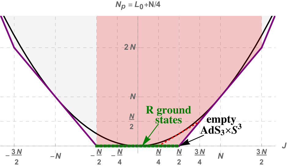 Figure 1
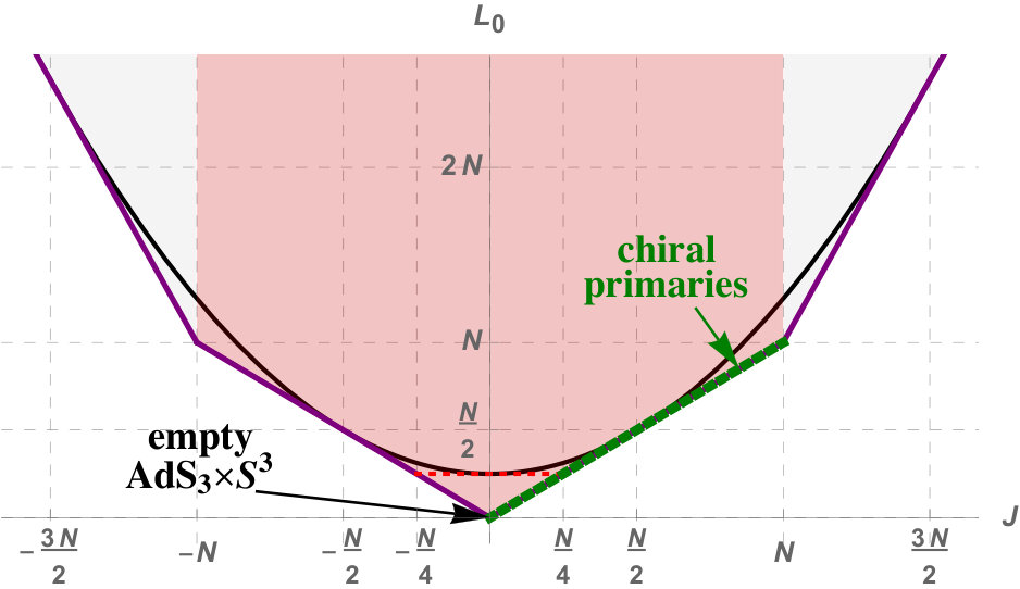 Figure 2
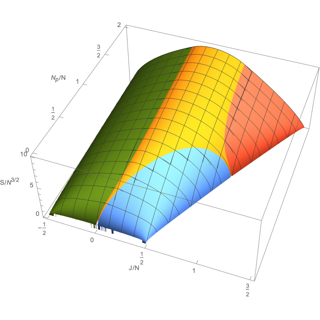 Figure 3
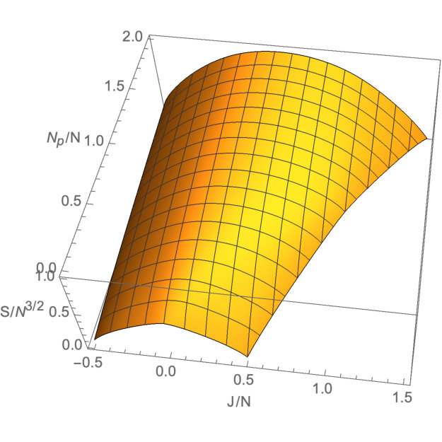 Figure 4
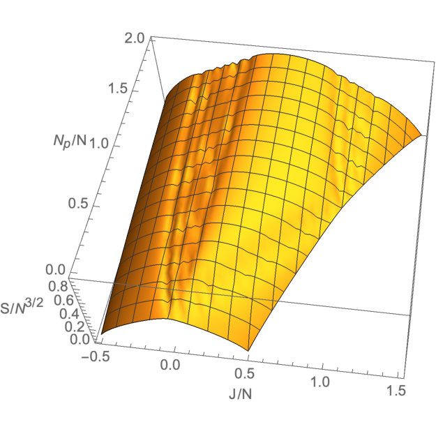 Figure 5
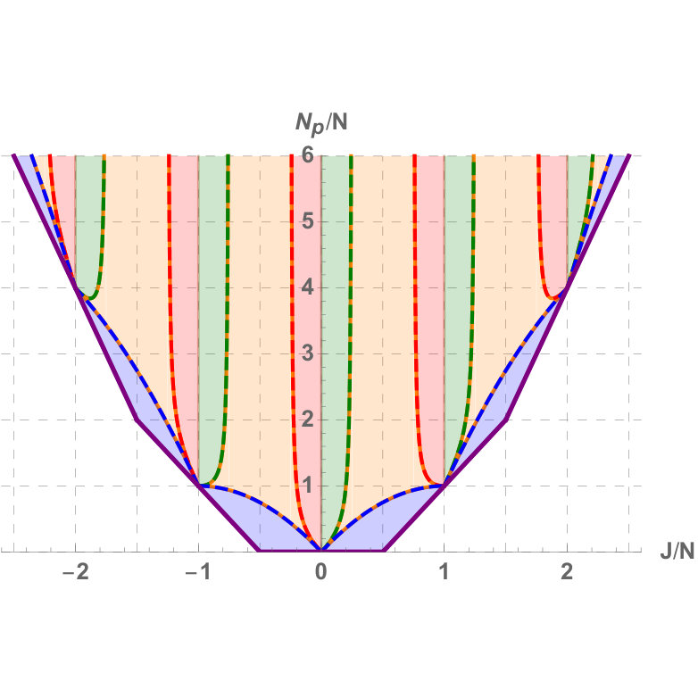 Figure 6
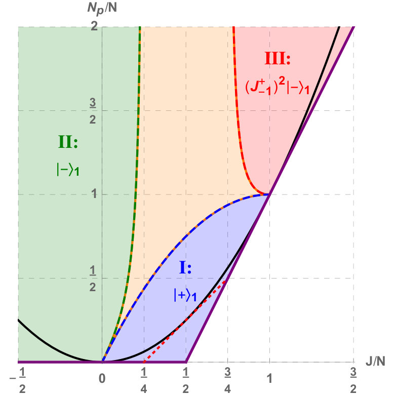 Figure 7
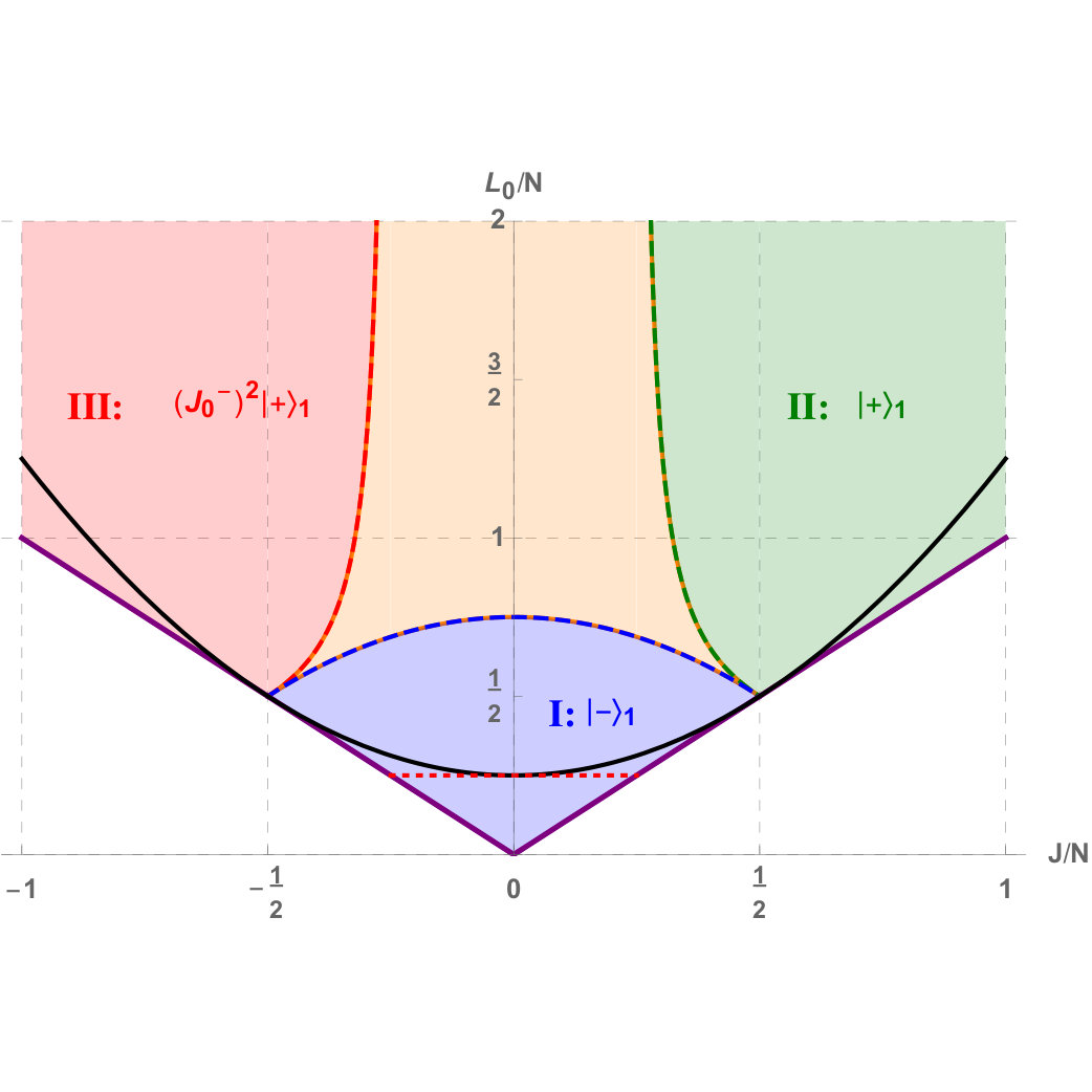 Figure 8
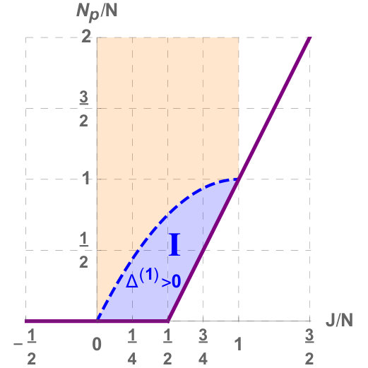 Figure 9
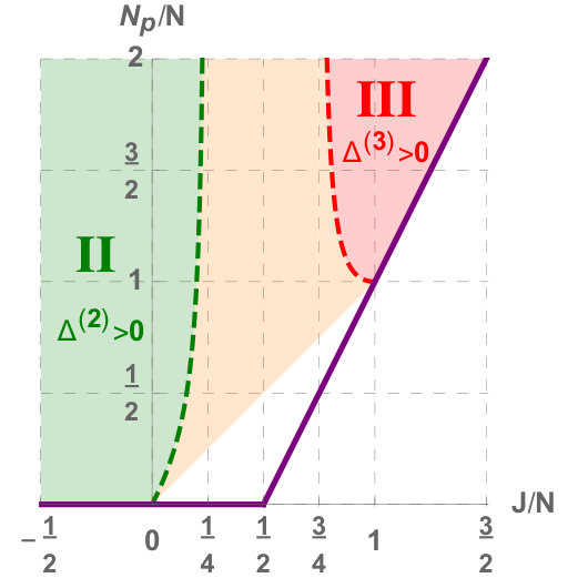 Figure 10
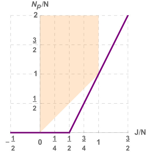 Figure 11
Peer Reviews
No public reviews on file for this paper yet. If you reviewed it on a platform where reviews are public (OpenReview, ICLR, NeurIPS, ICML), you can paste yours below so the community can read it here.
Videos
No videos yet. Explain this paper in a talk, walkthrough, or lecture? Add one.
YITP-19-61
Counting Superstrata
Masaki Shigemori
Department of Physics, Nagoya University, Furo-cho, Chikusa-ku, Nagoya 464-8602, Japan
and
Yukawa Institute for Theoretical Physics (YITP), Kyoto University
Kitashirakawa Oiwakecho, Sakyo-ku, Kyoto 606-8502 Japan
We count the number of regular supersymmetric solutions in supergravity, called superstrata, that represent non-linear completion of linear fluctuations around empty . These solutions carry the same charges as the D1-D5-P black hole and represent its microstates. We estimate the entropy using thermodynamic approximation and find that it is parametrically smaller than the area-entropy of the D1-D5-P black hole. Therefore, these superstrata based on are not typical microstates of the black hole. What are missing in the superstrata based on are higher and fractional modes in the dual CFT language. We speculate on what kind of other configurations to look at as possible realization of those modes in gravity picture, such as superstrata based on other geometries, as well as other brane configurations.
1 Introduction and summary
The D1-D5 system plays a central role in the string-theory understanding of microscopic physics of black holes. This system is obtained by compactifying type IIB string theory on with or K3 and wrapping D1-branes on and D5-branes on . If we add a third charge, units of Kaluza-Klein momentum (P) charge along , we have a 1/8-BPS, 3-charge black hole with a finite entropy which can be reproduced by microstate counting in the brane worldvolume theory [1]. More generally, we can also add left-moving angular momentum and the area entropy of the resulting 1/8-BPS black hole (the BMPV black hole [2]) is given by111 in our convention.
[TABLE]
Counting microstates in the brane worldvolume theory does not give us much information about their physical nature in the gravity (bulk) picture. Motivated by Mathur’s fuzzball conjecture [3, 4], a lot of endeavor has been made to construct microstates of black holes, especially of the D1-D5-P 3-charge black hole in the form of “microstate geometries”, namely, smooth horizonless solutions of classical supergravity.222Mathur’s conjecture per se does not claim that general microstates are describable within classical supergravity. The microstate geometry program is about how far one can go with classical supergravity. In this paper, we will restrict ourselves to BPS microstate geometries, which are in good theoretical control. In the 2-charge case where , the microstates can be realized in supergravity as the so-called Lunin-Mathur geometries [5, 6, 7, 8], which are parametrized by functions of one variable. The growth of the microscopic entropy, , can be reproduced by counting Lunin-Mathur geometries [9, 10], although the 2-charge system has vanishing area entropy at the classical level. In the 3-charge case, for which the area entropy is non-vanishing at the classical level, many families of microstates have been constructed based on the multi-center solutions [11, 12, 13, 14] (see [15, 16] about smooth multi-center solutions) and other methods, such as solution-generating technique, the matching technique, and BPS equations [17, 18, 19, 20, 21, 22, 23, 24, 25, 26, 27].
More recently, based on a linear structure of BPS equations in 6D supergravity [28], a new class of microstate geometries called superstrata was constructed [29, 30, 31, 32, 33, 34, 35, 36]. Superstrata are microstate geometries of the 3-charge D1-D5-P black hole, parametrized by functions of three variables, and their CFT duals are explicitly known. In essence, superstrata are non-linear completion of the linear excitations around empty AdS, which are sometimes called “supergravitons”. In other words, superstrata represent coherent states of the supergraviton gas with backreaction.
Because superstrata represent the largest known class of microstate geometries for the 3-charge black hole, it is of natural interest to count them and compute their entropy. In this paper, we carry out such computation and find an explicit formula for the entropy for large , . The explicit functional form of turns out to be quite complicated because, depending on the values of and , different bosons condense, which leads to different functional forms of . The explicit formulas are given in section 4.5. One interesting regime is the Cardy regime, .333Note that we have already taken the large limit. So, this means . In particular, for , we find that the entropy behaves as
[TABLE]
On the other hand, (1.1) gives
[TABLE]
which is parametrically larger than (1.2). Outside the Cardy regime, the behavior of the superstrata entropy is not simple, but its parametric growth for has the following universal form:
[TABLE]
Therefore, superstrata around AdS, although parametrized by functions of three variables, have parametrically smaller entropy than the 3-charge black hole. This is actually expected, because superstrata around AdS involve no higher or fractional modes that are important for reproducing the black-hole entropy [37, 29, 30].
The result (1.4) does not yet necessarily mean that supergravity solutions are insufficient for reproducing the black-hole entropy (1.1). What we counted in (1.4) are superstrata obtained by putting supergravitons in empty AdS, but there also exist superstrata that correspond to putting supergravitons in different backgrounds. In particular, in [30], superstrata on backgrounds were constructed, and those superstrata include some of fractional excitations, which we just said are important ingredients in order to reproduce the black-hole entropy in gravity picture. Therefore, the result (1.4) is better interpreted as suggesting where the microstate geometry program must go, for it to have any chance of succeeding in reproducing the black-hole entropy;444One could also consider superstrata on backgrounds with more than non-trivial 3-cycles but, according to the recent work [38], they would correspond to microstates of multi-center black holes, which do not exist everywhere in the moduli space and thus are not counted by a supersymmetric index. one must seriously look into solutions involving higher and fractional excitations, not only the ones in [30] but also more general ones. We will discuss what kind of configurations to look at in more detail in section 5.
Our working assumption in computing the entropy for superstrata is that their geometric quantization will exactly give the Hilbert space of supergravitons in the AdS background, with an appropriate stringy exclusion principle imposed. This is a very natural and safe assumption from the proposed holographic dictionary for superstrata [29, 31, 30], which is almost obvious from the construction and has passed some non-trivial test [39]. Under this assumption, we can count superstrata simply by counting states in the supergraviton Hilbert space, or equivalently, counting CFT states dual to them. More precisely, we compute the relevant partition function and estimate it for large using thermodynamic approximation, obtaining the result (1.4).
Let us very briefly recall the structure of the states of the D1-D5-P system. In the decoupling limit, the D1-D5 system is dual to a 2-dimensional boundary CFT called the D1-D5 CFT with central charge , as will be discussed in more detail later. We can talk about the microstates of the D1-D5-P system in the language of this CFT.
In the Ramond (R) sector of the CFT, on the - plane, states exist only in the region bounded below by the unitarity bound (the purple polygon in Figure -479). Here, and are Virasoro generators. This is only for the left-moving sector, but the right-moving sector is similar. The empty corresponds to the point . We can think of other states as excitation of this state. The 2-charge states corresponds to going horizontally to RR ground states on the interval , (the green dashed line in Figure -479). The 3-charge states correspond to going to . The 3-charge BMPV black hole exists only above the parabola , which is finitely away from the empty point. States representing superstrata obtained by exciting supergravitons on exist in the red shaded region in Figure -479.
We can map these states in the R sector into the ones in the Neveu-Schwarz (NS) sector by the spectral flow. We actually combine the spectral flow with the symmetry and use the map (2.9) to go between the R and NS sectors. The states in the R sector in Figure -479 are mapped into the NS sector in Figure -478 where the - diagram is shown. The empty corresponds to the ground state at the origin , while 2-charge states are chiral primaries on the line (green dashed line).
In the above, we talked about states in the range for the R sector and for the NS sector. However, by spectral flow we can get superstrata outside these ranges; see section 4.7 and appendix A for more detail.
The organization of the rest of the paper is as follows. In section 2, we review some relevant aspects of the D1-D5 CFT, in particular the structure of BPS states that can be interpreted as the states of a gas of supergravitons in the background. In section 3, we discuss superstrata solutions that have been explicitly constructed thus far, and argue that counting general superstrata in is the same as counting the states discussed in section 2. In section 4, we compute the partition function for the superstrata in and estimate its entropy in the large charge limit. We first compute the partial contributions that constitute the partition function and then put them together to construct the full partition function. See section 4.5 for the explicit formulas for the full entropy. We find that the entropy is parametrically smaller than the area-entropy of the D1-D5-P black hole. In section 5, we speculate on what kind of gravity configuration is relevant for the microstates of the D1-D5-P black hole.
2 CFT side
2.1 NS sector
Type IIB superstring on AdS, where or K3, is dual to a CFT called the D1-D5 CFT.555For reviews of the D1-D5 CFT, see e.g. [40, 41]. The symmetry group of this theory is , which is generated by the generators and their right-moving versions . Here, is a doublet index and is a triplet index for , while are their right-moving counterparts. The index is the doublet index for an additional symmetry group which acts as an outer automorphism on the superalgebra. In its moduli space, the D1-D5 CFT is believed to have an orbifold point where the theory is described by a supersymmetric sigma model with the target space being the symmetric orbifold .
In the NS-NS sector, the theory has one-particle chiral-primary states which are in one-to-one correspondence with the Dolbeault cohomology of [42, 43]. For , we have 16 species of states
[TABLE]
where . are doublet indices for an that is not part of the symmetry group of the theory. are the values of , while are those of . At the orbifold point, these states are twist operators of order ; namely, they intertwine copies of (out of copies). We refer to these copies, thus intertwined together, as a strand of length . Because spin is , the states are bosonic while are fermionic. The -invariant linear combination is denoted by . For K3, there are 24 species of one-particle chiral primary states and they are all bosonic:
[TABLE]
All these states (2.1), (2.2) preserve 8 supercharges, 4 from the left and another 4 from the right.666Except for the case with () and for which 8 left-moving (right-moving) supercharges are preserved. Conventionally, they are said to be 1/4-BPS, relative to the amount of supersymmetry (32 supercharges) of type IIB superstring in ten dimensions.
Among the states in (2.1), (2.2), the state is special because it has and represents the vacuum (of a single copy of ). All other states can be thought of as excitations and, via AdS/CFT, correspond to the possible excitations in linear supergravity around empty AdS, called supergravitons. In other words, each of the chiral primaries (2.1), (2.2) (except ) is in one-to-one correspondence with a particular one-particle, 1/4-BPS state of the supergraviton propagating in the bulk AdS background [44, 42, 45, 46].
The general chiral primary states, which are the most general 1/4-BPS states, are obtained by multiplying together one-particle chiral primary states as
[TABLE]
where runs over different species in (2.1) or (2.2). The general chiral primary state is specified by the set of numbers , which correspond to the number of strands of species and length . The values that can take are if and if is fermionic. The strand numbers must satisfy the constraint that the total strand length must be equal to :
[TABLE]
In the bulk, the states (2.3) correspond to multi-particle, 1/4-BPS states of supergravitons (“supergraviton gas”). Namely, the states (2.3) span the Fock space of 1/4-BPS supergravitons, modulo the constraint (2.4). When (where ), the bulk picture of supergravitons propagating in undeformed AdS is no longer valid but the geometry becomes deformed by backreaction.
The chiral primary states in (2.1) and (2.2) are the highest-weight states with respect to the rigid symmetry and more general, descendant states in the multiplet can be obtained by the action of the rigid generators and . To preserve supersymmetry, we will only consider descendants obtained by the action of the left-moving generators . If we start with a chiral primary with , which we denote by , we generate the following states:
[TABLE]
Here, means a state with . The states in the second line are doubly degenerate, because we can use with either or to descend from the first line to the second. The third line has no such degeneracy because we can only descend from the first line with . More precisely, to get a genuinely new state, we must act instead with where is the value of for the chiral primary [41, 35]. Moreover, the number corresponds to the number of times we act on the state with . We denote the states thus obtained building on by777These states are not normalized.
[TABLE]
If the chiral primary is bosonic (fermionic), the states (2.6a) and (2.6c) are bosonic (fermionic) while the state (2.6b) is fermionic (bosonic). These states break all left-moving supersymmetry but preserve 4 right-moving supercharges. In the bulk, they correspond to one-particle, 1/8-BPS supergraviton states obtained by the bulk action of the rigid generators. Actually, it is known that these states exactly reproduce the complete spectrum of linear supergravity around AdS [44, 42, 45, 46].
Just as in the 1/4-BPS case, we can multiply together one-particle, 1/8-BPS states to construct a more general 1/8-BPS state:
[TABLE]
where so it covers all the three kinds in (2.6). If the state is bosonic (fermionic), (). The state (2.7) corresponds in the bulk to a 1/8-BPS state of the supergraviton gas. Namely, (2.7) spans the Fock space of 1/8-BPS supergravitons, modulo the constraint on .
2.2 R sector
By spectral flow transformation, we can map all the above statements into the R sector. By spectral transformation, the charges of a state on a strand of length are transformed as follows:
[TABLE]
If we take the flow parameter , NS states get mapped into R states. However, to match the convention of charges to that in papers such as [29, 31, 33], we further flip the sign of the charge, as . So, the map from NS to R that we will be using is
[TABLE]
The same transformation to the right-moving sector is understood.
The map (2.9) transforms one-particle chiral primaries into R ground states on a strand of length . For example,
[TABLE]
The general R ground states, which are general 1/4-BPS states, are
[TABLE]
where runs over the species in (2.1) or (2.2), now understood as R ground states on a strand of length . Coherent superpositions of these supergraviton states are dual to smooth 1/4-BPS geometries called Lunin-Mathur geometries [5, 6, 7, 8], as mentioned in the introduction.
The 1/8-BPS states in the NS sector, (2.7), map into the R states of the following form:
[TABLE]
where now the one-particle supergraviton states are given by
[TABLE]
The operators acting on the R ground states have charges that have been shifted and sign-flipped due to spectral flow. The states (2.12) are realized as superstrata in the bulk, as we will expand in the next section.
2.3 Higher and fractional modes
From CFT, it is clear that the states (2.7) (or the R version (2.12)) we constructed above are not the most general 1/8-BPS states, because we used only the rigid generators, . We could act with higher generators with . On a stand of length , we could also act with fractional generators . However, these are not included in the states (2.7) (or (2.12), with the mode numbers of the generators appropriately shifted). Actually, it is known that, once we turn on perturbation and leave the orbifold point of the D1-D5 CFT [47], many of such higher/fractional states lift (see [48] for a more recent discussion) and disappear from the BPS spectrum. Nevertheless, there are ones that do not lift and are important to account for the entropy of the 3-charge black hole.
Actually, we can ask if the supergraviton states (2.7) (or (2.12)) also disappear when we leave the orbifold point of the D1-D5 CFT. For , we can see that these supergraviton states do not lift because they make non-vanishing contribution to the supersymmetric index (elliptic genus) [49]. This in particular means that, at any point in the moduli space of K3 surfaces,888The moduli space of K3 surfaces is part of the moduli space of the D1-D5 CFT, which also includes moduli corresponding to the NS-NS and RR fields through the K3. there are 1/8-BPS supergravitons in linear supergravity around . For , on the other hand, we cannot use an argument based on the supersymmetry index (the modified elliptic genus) because supergravitons do not contribute to it (at least for ) [50]. However, recall that, at the orbifold points in the moduli space of K3 surfaces, K3 is realized as () [51].999These orbifold points in the moduli space of K3 surfaces are not to be confused with the orbifold points in the moduli space of the D1-D5 CFT where the CFT target space is a symmetric orbifold of the K3 surface. As we just mentioned, the BPS spectrum of linear supergravity for this is non-empty. This means that the BPS spectrum of linear supergravity for the parent is also non-empty and presumably completely unlifted.101010Some modes (the ones associated with the fermionic chiral primaries) in the spectrum gets projected out by the orbifold action, while the K3 spectrum contains extra modes that come from the 16 collapsed 2-cycles at the fixed points of the orbifold. The overlap in the spectra (the modes associated with the bosonic chiral primaries of ) do not lift. The fact that the modified elliptic genus for vanishes most likely means that the modes associated with the fermionic chiral primaries do not lift either, responsible for the cancellation. Namely, even for , there exist BPS supergravitons and thus superstrata that are counted in this paper, even away from the orbifold point, for the values of the moduli for which can be orbifolded to give K3 [51].
3 Superstrata
Superstrata are regular horizonless 1/8-BPS solutions of supergravity that describe microstates of the D1-D5-P black hole. They are dual to coherent superpositions of the 1/8-BPS states (2.12) of the supergraviton gas and fully take into account the backreaction for .
More precisely, the superstrata that have been explicitly constructed thus far are believed to involve macroscopic excitation of the following species of one-particle supergravitons:111111Actually, there are superstrata that do not correspond to supergraviton states (2.12) obtained by exciting supergravitons around AdS. In [30], superstrata solutions were written down that are obtained by exciting supergravitons around an orbifold background . The dual CFT states involve certain fractional generators and cannot be written in the form (2.12).
- •
: the “original” superstratum [29, 31, 33].
- •
: “style 1” [30].
- •
: superstratum with internal excitations[34].
- •
: supercharged superstratum [35].
- •
: “hybrid” superstratum [36].
In addition, these all involve which corresponds to the vacuum in the NS sector.
These superstrata solutions were constructed relying on a linear structure that the BPS equations of 6D supergravity possess [28]. In particular, these solutions have a flat four-dimensional base on which the BPS equations are defined. If one considers more general species, such as , the base gets deformed and it becomes more difficult to construct backreacted supergravity solutions by making use of the linear structure. However, this is only a technical issue, and it is physically natural to expect that, for every species , there exists a smooth backreacted solution (superstratum) that corresponds to a macroscopic, coherent excitation of the corresponding supergraviton. Below, we assume that we can identify the states (2.12) with such general superstrata, and that geometric quantization of the latter will reproduce the Hilbert space of states (2.12). Under the assumption, we now count superstrata by counting the states (2.12).
Note that the “stringy exclusion principle” constraint [42] such as the second equation of (2.12) has been observed to be automatically imposed in fully backreacted geometries, such as superstrata [29], as regularity constraint [52]. Therefore, we assume that counting the states (2.12) including the constraint is the same as counting all regular superstrata.
4 Counting
In this section, we carry out the counting of the number of states (2.12), which we assume to be the same as counting the dual superstrata solutions. More precisely, we will compute the 1/8-BPS grand-canonical partition function
[TABLE]
where and the trace is over the Fock space states in the R sector, (2.12), for given . We do not have to consider the constraint on the total strand length in the grand-canonical partition function since it is taken care of by the strand-length counting parameter . Note that, due to the shift by in the definition (4.1), the power of records not the value of but
[TABLE]
which vanishes for R ground states.
4.1 The partition function
To compute , it is perhaps easiest to go back to the NS sector and start with the contribution of the states in (2.5) to an NS sector grand-canonical partition function. If the chiral primary is a bosonic state, the contribution to the partition function from it and from its descendants is
[TABLE]
The two factors in the denominator come from the first and third lines of (2.5), while the numerator comes from the second line of (2.5). The product over comes from the action of and the product of from the action of . This (4.3) represents the contribution of multi-particle states of supergravitons, built on with the particular string length, . By using the standard technique of taking the logarithm and using the formula , we can carry out the summation over and , obtaining
[TABLE]
Note that this does not depend on . This expression is valid for states built on bosonic chiral primaries in (2.1) and (2.2), namely , , and , which have
[TABLE]
Summing over all possible strand length, , we obtain the contribution from the states of species :
[TABLE]
Here, we used the notation because this depends only on the value of of the chiral primary. We will often suppress the right-moving part of the states, which is irrelevant, and write e.g. as and as .
Let us translate this into the R sector. By inspecting the transformation (2.9), one sees that the NS partition function can be converted into the R partition function by the replacement
[TABLE]
Here, we have also taken into account the fact that we have defined the R partition function (4.1) with the shift . By applying this to (4.6), we find that the contribution to from states built on the bosonic R ground state with is
[TABLE]
where we omitted the superscript “R” for the R sector, because we will only be discussing R sector quantities henceforth.
Similarly, if the R ground state is fermionic and has , the contribution from states built on it is
[TABLE]
Summing (4.8) and (4.9) over all the species in (2.1) and (2.2), we finally obtain the grand-canonical partition function for and K3 as follows:
[TABLE]
Our goal is to estimate these partition functions to estimate the number of states.
4.2 Thermodynamic approximation
Let us expand the partition function as
[TABLE]
What we would like to know is the behavior of the coefficient in the large charge limit,
[TABLE]
Note that and are large and positive, while can be as large as . So, can be either positive, negative, or zero. We introduce the chemical potentials by
[TABLE]
where while can be positive, negative, or zero. In the limit (4.12), we have
[TABLE]
where indicates how fast are going to zero. In the large charge limit, we can use thermodynamic approximation, within which we have
[TABLE]
and entropy is given by
[TABLE]
4.3 Warm-up: a 2-charge system with angular momentum
Before estimating the 3-charge partition function of supergravitons, it is instructive to look at 2-charge partition function to gain an idea.
Consider a 2-charge ensemble made of states of the form
[TABLE]
Namely, we have only one species of strands, carrying angular momentum , with no excitation on top. The partition function for this system is
[TABLE]
If we also included strands, this could be related to theta functions and could be estimated using modular properties of theta functions [53], but we will not do so but take a thermodynamic approach.
As before, (4.18) can be written as
[TABLE]
In the large limit where , one may wonder if we can simply plug in (4.13) to obtain
[TABLE]
However, this is incorrect as the formula (4.15) would always give .
What went wrong is physically clear: if , the strand condenses, because that is the most economical way to carry angular momentum. This is manifested in (4.19) in the fact that the sum diverges if , which happens if . If we extract the dangerous contribution from the partition function (4.18) and rewrite the rest as an -sum, we find
[TABLE]
Note that is not dangerous even if . Then, by a straightforward application of the thermodynamic formulas, we find
[TABLE]
Therefore, , while . The entropy is
[TABLE]
where we dropped subleading terms (such as ). This is a well-known 2-charge entropy formula [54].
Some comments are in order. (i) In this example, because all strands have , there is no state with and therefore it must be that as . However, this is invisible in (4.23), which is valid only in the large limit. (ii) We said that a condensate of absorbs . Strictly speaking, we do not have but with . The remaining strand-length budget of order is occupied by strands of average length and is responsible for the entropy. The spin carried by these strands () is negligible compared to that of the condensate (). One can show that . (iii) More generally, if we have species of carrying and species of with , entropy becomes , . Depending on , the strand condenses.
4.4 Estimating building blocks
Now let us come back to the estimation of the 3-charge partition function of superstrata/supergravitons. Before estimating the entropy for the full partition function (4.10), it is useful to first estimate the individual contributions, such as .
4.4.1 Case 1:
Let us start with . Namely, we expand as
[TABLE]
and want to estimate the behavior of in the large charge limit.
If we set in (4.8), plug in (4.13), and expand the summand according to (4.14), we obtain
[TABLE]
Ignoring the terms and carrying out the summation over , we obtain
[TABLE]
where we have defined
[TABLE]
If we introduce conjugate to by
[TABLE]
then the thermodynamic relations (4.15) and (4.16) become
[TABLE]
and
[TABLE]
In the present case, using (4.26) and (4.29), we find
[TABLE]
and the entropy is
[TABLE]
Because , in order for the entropy to be positive, we need and therefore . It is also clear that . In terms of , we need
[TABLE]
See Fig. -477 for the region where .
The relations (4.31) can be solved for as
[TABLE]
which gives the entropy of in terms of charges to be
[TABLE]
4.4.2 Case 2:
Let us turn to . Just as in the 2-charge case studied in section 4.3, in an ensemble of strands with angular momentum, condensation of the shortest-length strand is expected when is large (see [55, 54]). We will indeed see such condensation in this case.
By setting in (4.8), we find
[TABLE]
If we naively do small- expansion of the summand, as we did for , then we get the same expression (4.26) and the same entropy (4.35). However, such expansion is not always valid. In the numerator of (4.36), we have . So, for the series to converge, we need
[TABLE]
where in the “” we used (4.34). However, this inequality is not always satisfied.121212On the other hand, if it is satisfied, other quantities in the numerator, such as are all strictly smaller than one and the series converges.*,*131313More precisely, the left-hand side can go to zero faster than , just as for the 2-charge case studied in section 4.3. When the left-hand side of (4.37) becomes very small, the expansion of the summand that led to (4.26) is no longer valid. This is because the state counted by , namely, , condenses.
Let us focus on the first term in (4.36) and extract terms that become large when the left-hand side of (4.37) becomes very small. Using , we can rewrite it as
[TABLE]
The second term on the right is safe, as long as . On the other hand, the first term can be rewritten as
[TABLE]
The terms give:
[TABLE]
while other () terms give contributions which are subleading compared to (4.26). The remaining terms in (4.36) and the second term in (4.38) give (4.26), just as for the case with . So, the partition function is given by
[TABLE]
Using thermodynamic relations (4.29), we obtain
[TABLE]
where
[TABLE]
The two terms on the right-hand side of (4.42) are of the same order if
[TABLE]
The entropy is computed to be
[TABLE]
where we have dropped subleading terms, including the term that comes from the first term in (4.41).
Looking at the definition of in (4.28), we see that the existence of the terms in (4.42) change by and by . This means that we have the following condensate:
[TABLE]
In order to express the entropy in terms of charges, let us define
[TABLE]
Then (4.42) become
[TABLE]
which have the same form as (4.31) and we immediately obtain
[TABLE]
and
[TABLE]
On the other hand, the condition means that
[TABLE]
which we can solve to find in terms of . The solution is
[TABLE]
With this sign choice in front of the square root, the region in which is
[TABLE]
We also included inequalities (the second and third ones) which come from the condition required for the entropy to be positive, as in the case for . This region (4.53) is in the complement of the region given by (4.37). The condensate vanishes when the first inequality in (4.53) is saturated. In Fig. -476, region I is displayed in blue.
One may wonder that, if we send in the entropy formula (4.50), we can recover the 2-charge entropy (4.23). However, this does not happen because the regime of parameters is different; the 3-charge formula (4.50) is valid only for , while the 2-charge formula (4.23) is valid only for .
4.4.3 Case 3:
In this case, we expect that condenses. The partition function is, from (4.8),
[TABLE]
This time, the naive small- expansion of the summand and the results (4.26) and (4.35) becomes invalid if is too close to . So, the validity region of the naive result is
[TABLE]
If the left-hand side becomes very close to zero, the strand counted by , namely , condenses. By a computation very similar to the case for , we find
[TABLE]
Using (4.29), we get
[TABLE]
where now
[TABLE]
The terms in (4.57) change by and by . This means that we have the following condensate:
[TABLE]
If we define, just as in (4.47),
[TABLE]
then are given by (4.49), with the superscript “(1)” replaced by “(2)”. Again, is determined by the condition , which amounts to
[TABLE]
This gives
[TABLE]
A choice for the sign has been made just as for the case with . The region in which is in the complement of the region given by (4.55), namely,
[TABLE]
Here, we also included inequalities that come from the condition . In Fig. -475, region II is displayed in green. The entropy in this region is given by the same expression as before, Eq. (4.50), with “(1)” replaced by “(2)”.
We just found that condensation occurs in the region with . Recall that we have spectral flow symmetry (2.8) and the charge-flipping symmetry . Combining these, we can show that there is symmetry that maps states with into those with . More precisely, flowing from the R sector to the NS sector, flipping the sign of there, and then flowing back to the R sector, we have the following map on a strand of length :
[TABLE]
Under this map, with goes to with . This means that, there must be a region with where condenses.141414In the NS sector, corresponds to a chiral primary with , while corresponds to an anti-chiral primary with .
The map (4.64) can be realized in the partition function by the replacement
[TABLE]
It is straightforward to show that (4.54) is invariant under this. In particular, the very first term involving , which led to condensation of , is mapped into . When this is very close to one, the partition function is
[TABLE]
So, this time,
[TABLE]
where now
[TABLE]
The terms in (4.67) change by , by , and by . This means that we have the following condensate:
[TABLE]
If we define
[TABLE]
then are given by (4.49), with the superscript “(1)” replaced by “(3)”. is determined by the condition , which amounts to
[TABLE]
This gives
[TABLE]
The region in which is given by
[TABLE]
Here, we also included inequalities that come from the condition . In Fig. -475, region III is displayed in red. The entropy in this region is given by Eq. (4.50), with “(1)” replaced by “(3)”.
4.4.4 Case 4:
Lastly let us consider the fermionic case. Because the terms that were dangerous for the bosonic case, namely the very first term and the very last term in (4.8), come with alternating signs in the fermionic partition function (4.9), these terms do not lead to divergences. This means that the naive small- expansion of the summand of the fermionic partition function (4.9) is always justified and we obtain
[TABLE]
independent of the value of . Note that this is identical to the “bosonic” result, (4.26), without that one might have expected for a “fermionic” partition function. This is because the descendant states we are counting always include both bosonic and fermionic states, whether the R ground state on which these states are built is bosonic or fermionic. Namely, if is bosonic (fermionic), the first and third lines of (2.13) are bosonic (fermionic) and the second line of (2.13) are fermionic (bosonic).
4.5 Entropy for the full partition function
Let us put together the pieces obtained above and estimate the entropy for the full partition function (4.10). A naive small- expansion of the summand gives
[TABLE]
where was defined in (4.26) and
[TABLE]
Just as for discussed in section 4.4.1, the entropy is computed to be
[TABLE]
where were defined in (4.28). However, this expression is not valid for all values of , due to condensation of certain length-one strands.
In region I defined by (4.53), (more precisely, the left-hand side becomes ) due to the condensation of the strand . The partition function in this case is modified from (4.75) as
[TABLE]
The condensate has the following form:
[TABLE]
where we defined
[TABLE]
(the factor as compared to (4.43) is due to the 2 in front of in (4.10)). The entropy in region I is
[TABLE]
where are defined by (4.47) and is given by (4.52).
In region II defined by (4.63), due to the condensation of the strand . The partition function in this case is
[TABLE]
The condensate is
[TABLE]
The entropy in region II is
[TABLE]
where are defined by (4.60) and is given by (4.62).
In region III defined by (4.73), due to the condensation of the strand . The partition function in this case is
[TABLE]
The condensate is
[TABLE]
The entropy in region III is
[TABLE]
where are defined by (4.70) and is given by (4.72).
In Fig. -474, different regions on the - plane are displayed. In regions I–III, certain condensate forms and one must use different formulas (Eqs. (4.77), (4.81), (4.84), and (4.87)). In Fig. -473, a plot of the entropy is given, for the case with . As one can see, the entropy as a function of is smooth across the boundary of different regions. The case is identical, except for the overall factor due to difference in the value of .
The general formulas for entropy are complicated, but for some special cases they simplify. For large ,151515 See footnote 3. region I becomes irrelevant while regions II and III become vertical strips on the - plane. The entropy for this regime is given by
[TABLE]
One can also consider the entropy for . This is entirely in region II and the entropy is
[TABLE]
This behaves for small and large as161616Because we have already taking the large limit, this means that and .
[TABLE]
4.6 Comparison with the black-hole entropy
In the above, we derived the entropy of the ensemble of supergravitons, or equivalently, superstrata. Although the precise functional form depends on the region on the - plane, we universally have
[TABLE]
This is parametrically smaller than the black-hole entropy,
[TABLE]
Namely, as expected, superstrata obtained by non-linear completion of supergraviton gas states around empty AdS have much less entropy than the black hole.
In (4.88), we estimated the entropy for . In that case, we obtain
[TABLE]
while, in the same regime,
[TABLE]
So, the superstrata are too few because of the smaller power of .
In [12], the entropy of the possible microstate geometries in the D1-D5 system was estimated based on the entropy enhancement mechanism. This mechanism says that the entropy carried by supertubes is strongly enhanced by putting them in the throat of a smooth multi-center solution [15, 16]. Because supertubes can become smooth geometries upon backreaction [5, 6], the entire configuration is expected to become a smooth geometry. This mechanism is expected to lead to microstate geometries with a large entropy. The estimate of [12, Eq. (6.18)] is that, if then the entropy is . This agrees with (4.93) if we set . However, the scaling regime appear to be different and it is not clear if this is a sensible comparison. We leave for future research a further investigation into this interesting issue.
4.7 Spectral flows
In the above, we considered the states of the form (2.12), which are within the range . However, by spectral flow (2.8), we can map these states into other range. For example, by spectral flow with , we obtain states that sit within the range . More generally, the states spectral-flowed by parameter sit in the range . These states do not describe fluctuations around empty AdS but are fluctuations around spectral flows of empty AdS. However, the corresponding superstrata solutions do represent microstate geometries as the original (unflowed) superstrata do and their entropy must also be taken into account. The entropy of the spectral-flowed states can be easily obtained by applying the spectral flow (2.8) to the entropy formulas obtained in section 4.5. Let us discuss how the phase diagram in Fig. -474 changes if we consider such spectral-flowed states.
The interval overlaps with in the range . In the overlapping region, one can show that the entropy of the -flowed states is dominant in while the entropy of the -flowed states is dominant in . This means that the -flowed states are dominant for . Actually, if we take the symmetry also into account, the boundary between different regions of dominance can not be anywhere else than , .
The regions of dominance on the - plane, taking into account flowed states, are shown in Fig. -472. The meaning of the colors is the same as that in Fig. -474. In the flows of regions I, II, and III (blue, green, and red), the flows of the states , , and condense, respectively.
5 Discussion
In this paper, we evaluated the partition function of CFT states that correspond to superstrata in the bulk. These superstrata can be thought of as non-linear completion of supergravitons around empty AdS, and represent a certain class of microstates of the D1-D5-P black hole. We found that the entropy computed from the partition function is parametrically smaller than the entropy of the black hole with the same charges. Therefore, these superstrata based on are not typical microstates of the black hole.
Our result is similar to [52], in which gravity microstates (multi-center solutions) of a certain 4-charge system were counted and the entropy was found to be parametrically smaller than the corresponding black-hole entropy. Instead, the entropy was found to be equal to that of the supergraviton gas in an AdS3 background. However, what is different in our setup compared to that in [52] is that we have a boundary CFT which is in a better theoretical control and gives us hints as to what kind of state we are missing. The ingredients that the superstrata counted in this paper lack are higher and fractional modes. The superstrata constructed in [30] involve some fractional modes because they are not based on but on the orbifold . It would be interesting to generalize the counting of the current paper to include such superstrata.171717One would have to be careful to the fact that some supergravitons on with different values of actually represent the same state. However, the class of fractional modes that these superstrata [30] involve are restricted and we must look for the bulk realization of states involving more general fractional modes and also higher modes.
At the orbifold point of the D1-D5 CFT, it is clear how to construct BPS states that involve higher and fractional modes. On a strand of length , we have modes such as with (in the NS sector) and we are free to excite them as long as the total on the strand is an integer. If we go away from the orbifold point, many of these states are known to lift and become non-BPS [47, 48]. The strand excited by generators with general mode numbers is conjectured to correspond to a string propagating in with string oscillators excited on it [56, 57, 47] (see also [58]). On the other hand, the modified elliptic genus for computed from CFT gets contribution only from “identical-strand” states, namely, one must have length- strands with identical excitations on every one of them [50]. This suggests that, a single string with oscillators excited on it is non-BPS away from the orbifold point but, if we have as many copies of the same string as is allowed by the stringy exclusion principle, they give rise to a BPS state because the binding energy cancels the excitation energy of the string oscillators (this statement was confirmed by an explicit CFT computation for a particular excited strand in [48]).
This seems to suggest that states involving general (higher and fractional) modes are represented in gravity picture by non-BPS strings propagating in some background. However, that is a picture valid for a small number of strings. If we have such strings, all in the same state, they are likely to have an alternative description in terms some puffed-out branes or backreacted geometries, by polarization due to Myers’ effect [59] or the supertube effect [60].181818Examples of such phenomena are common in string theory, including giant gravitons [61], which are gravitons polarizing into D-branes, or Wilson loops [62], which are fundamental strings on top of each other, being better described in terms of D-branes. Those D-brane configurations have a gravity description in terms of smooth geometries [63, 64]. Such brane configurations or microstate geometries may still be non-BPS, as the original (unpuffed-out) string, but it is logically possible that they actually become BPS in this alternative description in certain situations. Indeed, recall that, it was observed [55] that there is some correspondence between states that are BPS at the orbifold point of the D1-D5 CFT but become non-BPS away from the orbifold point, and solutions in supergravity that are BPS when moduli are trivial (internal NS-NS and RR fields vanish) but become non-BPS when generic moduli are turned on [65, 38]. Because these string states are BPS at the orbifold point, it is conceivable that the puffed-out strings are represented by some BPS configurations in supergravity when moduli are trivial. In this view, it would be interesting to study possible relations between such puffed-out branes and known BPS brane configurations in the D1-D5 system [66].
Another interesting background to look at is . It has been argued that the bulk microstates of BPS black holes live in the close vicinity of the horizon and are represented by asymptotically AdS2 configurations with vanishing angular momentum [67, 68, 69]. In the language of quiver quantum mechanics, they correspond to states in the so-called pure Higgs branch [70]. Recently, some pieces of evidence have been found for the relevance of microstate geometries with AdS2 asymptotics for black-hole microstates. In [71], certain configurations of codimension-two branes were explicitly constructed as candidates for black-hole microstates. Interestingly, such solutions can exist only with AdS asymptotics, due to the monodromic structure of the harmonic functions required of the codimension-two branes. These states have vanishing angular momentum due to a cancellation mechanism by interaction between branes. In a more recent paper [72], an exhaustive search for smooth multi-center solutions of type [15, 16] with minimum possible charges was carried out and, it was found that the bubble equations allow exactly as many solutions as predicted by the quiver quantum mechanics living on the branes [68, 69]. These solutions have no angular momentum and are all asymptotically AdS, which appears to suggest that states in the pure Higgs branch are represented by asymptotically AdS2 configurations in the bulk. Therefore, it would be highly interesting to study gravity microstates with D1-D5-P charges (superstrata or any other configurations, with or without supergravity description) imposing a strict AdS2 boundary condition at infinity. Having no AdS3 region makes it difficult to identify the corresponding dual state in the D1-D5 CFT, but considering an AdS2 limit of superstrata solutions with known CFT duals, such as [73], can be useful for that purpose.
In the current paper, we computed the partition function of supergravitons (or equivalently, superstrata). Another very interesting quantity to investigate is the (modified) elliptic genus. It was shown by de Boer [49] that the elliptic genus computed from CFT agrees with the elliptic genus computed by enumerating (with signs) supergravitons, for for K3 (for the modified elliptic genus for , the bound is [50]). This de Boer bound is shown as red dashed lines in Fig. -479 and other Figures. Above this bound, new primary states appear, which are responsible for the black-hole entropy. Above this bound and below the black-hole bound, , the CFT elliptic genus is different from the supergraviton elliptic genus but does not yet show a black-hole growth. It is quite interesting to study the behavior of the elliptic genera in this intermediate region to understand the nature of states that are not captured by supergravitons. The supergraviton elliptic genus is obtained simply by changing some signs in partition functions such as (4.3). However, because the coefficients of elliptic genus can be positive or negative, unlike partition function, we cannot use a thermodynamic approximation we used in this paper to estimate its growth. We probably need a more sophisticated way to rewrite the elliptic genus to be able to accurately estimate it, such as the one in [74] or its relation to four-dimensional indices [75]. In Fig. -471, we plotted the supergraviton partition function and the supergraviton elliptic genus for K3 for . We can see that the elliptic genus has structure more non-trivial than the partition function. If would be interesting to understand this structure.
Acknowledgments
I thank Iosif Bena, Jan de Boer, Pierre Heidmann, Stefano Giusto, Emil Martinec, David Turton, Rodolfo Russo and Nick Warner for useful discussions. The work of MS was supported in part by JSPS KAKENHI Grant Numbers 16H03979, and MEXT KAKENHI Grant Numbers 17H06357 and 17H06359.
Appendix A The NS sector
In the main text, we studied the entropy of the R states of the form (2.12), because bulk states naturally live in the R sector. In this Appendix, we discuss the NS sector formulas, which are obtained by applying the map (2.9) to the R formulas. Some formulas are simpler in the NS sector because of the symmetry.
If nothing condenses, the entropy in the R sector is given by (4.77), which becomes, in the NS sector,
[TABLE]
Region I, which was defined for the R sector by (4.53), is defined in the NS sector by
[TABLE]
and the entropy there is
[TABLE]
In region I, what condenses is , but this is nothing but the vacuum (of a single copy of ). So, in the NS sector, it is more appropriate to say that, in this region, the excitations have not yet fully occupied the copies.
Regions II and III, which were given for the R sector by (4.63) and (4.73), are defined in the NS sector by
[TABLE]
where the () sign is for region II (III). The entropy is
[TABLE]
See Fig. -470 for the phase diagram on the - plane in the NS sector.
If we take into account of the spectral flows, only the states above in the range are dominant. In the range , , the spectral-flowed states by the parameter are dominant.
The reference list from the paper itself. Each links out to its DOI / PubMed record.
- 1[1] A. Strominger and C. Vafa, “Microscopic origin of the Bekenstein-Hawking entropy,” Phys. Lett. B 379 , 99 (1996) doi:10.1016/0370-2693(96)00345-0 [hep-th/9601029].
- 2[2] J. C. Breckenridge, R. C. Myers, A. W. Peet and C. Vafa, “D-branes and spinning black holes,” Phys. Lett. B 391 , 93 (1997) doi:10.1016/S 0370-2693(96)01460-8 [hep-th/9602065].
- 3[3] S. D. Mathur, “The Fuzzball proposal for black holes: An Elementary review,” Fortsch. Phys. 53 , 793 (2005) doi:10.1002/prop.200410203 [hep-th/0502050].
- 4[4] S. D. Mathur, “The Information paradox: A Pedagogical introduction,” Class. Quant. Grav. 26 , 224001 (2009) doi:10.1088/0264-9381/26/22/224001 [ar Xiv:0909.1038 [hep-th]].
- 5[5] O. Lunin and S. D. Mathur, “Ad S / CFT duality and the black hole information paradox,” Nucl. Phys. B 623 , 342 (2002) doi:10.1016/S 0550-3213(01)00620-4 [hep-th/0109154].
- 6[6] O. Lunin, J. M. Maldacena and L. Maoz, “Gravity solutions for the D 1-D 5 system with angular momentum,” hep-th/0212210.
- 7[7] M. Taylor, “General 2 charge geometries,” JHEP 0603 , 009 (2006) doi:10.1088/1126-6708/2006/03/009 [hep-th/0507223].
- 8[8] I. Kanitscheider, K. Skenderis and M. Taylor, “Fuzzballs with internal excitations,” JHEP 0706 , 056 (2007) doi:10.1088/1126-6708/2007/06/056 [ar Xiv:0704.0690 [hep-th]].