Continuous time random walk and diffusion with generalized fractional Poisson process
Thomas M. Michelitsch, Alejandro P. Riascos

TL;DR
This paper analyzes the generalized fractional Poisson process (GFPP), develops related fractional diffusion equations, and explores its applications in modeling anomalous transport and complex system dynamics.
Contribution
It introduces a comprehensive analysis of GFPP, generalizes fractional Poisson models, and derives a new fractional diffusion equation for continuous time random walks.
Findings
GFPP includes Laskin's fractional Poisson as a special case
Derived a generalized fractional diffusion equation
Showed subdiffusive behavior with mean-square displacement ~ t^β
Abstract
A non-Markovian counting process, the `generalized fractional Poisson process' (GFPP) introduced by Cahoy and Polito in 2013 is analyzed. The GFPP contains two index parameters , and a time scale parameter. Generalizations to Laskin's fractional Poisson distribution and to the fractional Kolmogorov-Feller equation are derived. We develop a continuous time random walk subordinated to a GFPP in the infinite integer lattice . For this stochastic motion, we deduce a `generalized fractional diffusion equation'. In a well-scaled diffusion limit this motion is governed by the same type of fractional diffusion equation as with the fractional Poisson process exhibiting subdiffusive -power law for the mean-square displacement. In the special cases with the equations of the Laskin fractional Poisson process and for…
Click any figure to enlarge with its caption.
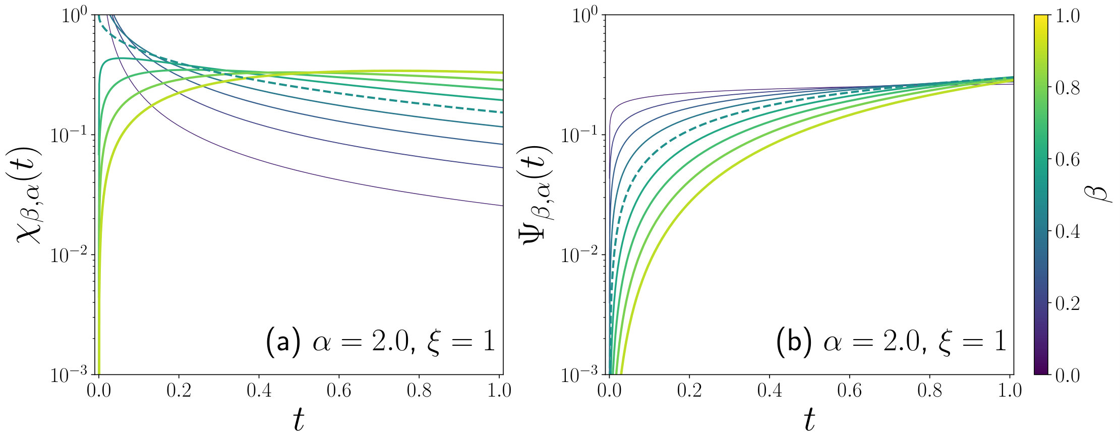 Figure 1
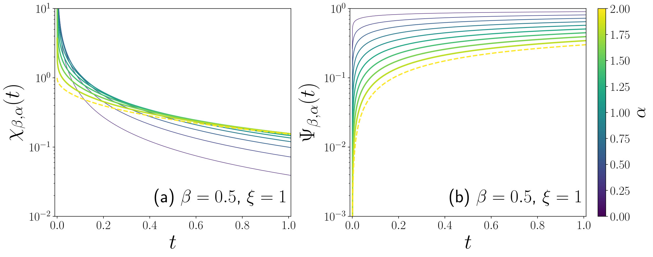 Figure 2
Peer Reviews
No public reviews on file for this paper yet. If you reviewed it on a platform where reviews are public (OpenReview, ICLR, NeurIPS, ICML), you can paste yours below so the community can read it here.
Videos
No videos yet. Explain this paper in a talk, walkthrough, or lecture? Add one.
Continuous time random walk and diffusion with generalized fractional Poisson process
Thomas M. Michelitsch1111Corresponding author, e-mail : [email protected] , Alejandro P. Riascos2
1 Sorbonne Université
Institut Jean le Rond d’Alembert, CNRS UMR 7190
4 place Jussieu, 75252 Paris cedex 05, France
2 Instituto de Física, Universidad Nacional Autónoma de México,
Apartado Postal 20-364, 01000 Ciudad de México, México
Accepted for publication in Physica A
Abstract
A non-Markovian counting process, the ‘generalized fractional Poisson process’ (GFPP) introduced by Cahoy and Polito in 2013 is analyzed. The GFPP contains two index parameters , and a time scale parameter. Generalizations to Laskin’s fractional Poisson distribution and to the fractional Kolmogorov-Feller equation are derived. We develop a continuous time random walk subordinated to a GFPP in the infinite integer lattice . For this stochastic motion, we deduce a ‘generalized fractional diffusion equation’. In a well-scaled diffusion limit this motion is governed by the same type of fractional diffusion equation as with the fractional Poisson process exhibiting subdiffusive -power law for the mean-square displacement. In the special cases with the equations of the Laskin fractional Poisson process and for with the classical equations of the standard Poisson process are recovered. The remarkably rich dynamics introduced by the GFPP opens a wide field of applications in anomalous transport and in the dynamics of complex systems.
*Keywords
Renewal process, fractional Poisson process and distribution, fractional Kolmogorov-Feller equation,
continuous time random walk, generalized fractional diffusion.*
1 Introduction
In many complex systems, one has empirically observed asymptotic power laws instead of the classical exponential patterns. One finds such characteristic behavior for instance in anomalous transport and diffusion [1, 2, 3, 4, 5, 6, 7]. In the description of these phenomena the celebrated Montroll-Weiss continuous time random walk (CTRW) model [2, 8, 9, 10] has become a major approach where the empirical power laws lead to descriptions that involve fractional calculus.
Meanwhile, the CTRW of Montroll and Weiss has been applied to a vast number of problems in various contexts especially to model anomalous diffusion and transport phenomena [2, 10, 11] including stochastic processes in protein folding [12], the dynamics of chemical reactions [13], transport phenomena in low dimensional chaotic systems [14], ‘Aging Continuous Time Random Walks’ [15, 16], CTRW with correlated memory kernels have been introduced [17], and many further applications of the CTRW exist. In the classical picture, CTRWs are random walks subordinated to a Poisson renewal process with exponentially decaying waiting time densities and the Markovian property [5, 6, 18]. However, one has found that many complex systems are rather governed by non-Markovian fat-tailed waiting time densities not compatible with the classical Poisson process picture [3, 5, 19, 20].
Based on a renewal process to our present knowledge first introduced by Repin and Saichev [21], Laskin developed a non-Markovian fractional generalization of the Markovian Poisson process. He called this process ‘fractional Poisson process’ [19] and demonstrated various important applications [22]. The fractional Poisson process is of utmost importance as it produces power-law patterns as observed in anomalous subdiffusion due to fat-tailed waiting time densities. Meanwhile, a large literature exists that analyze fractional Poisson processes and related random motions [4, 6, 23, 24, 25, 26, 27].
In the present paper, our aim is the development of a stochastic motion based on a generalization of the Laskin’s fractional Poisson process. This process was introduced by Cahoy and Polito in 2013 [28] and several features were analyzed in that paper. In the present paper, our goal is to complement that analysis and to investigate related stochastic motions. We call this renewal process ‘generalized fractional Poisson process’ (GFPP). Both the GFPP like the fractional Poisson process are non-Markovian and introduce long-memory effects. We will come back to this issue subsequently.
The present paper is organized as follows. In the first part (Section 2) we briefly outline general concepts of renewal theory and the CTRW approach by Montroll and Weiss [8, 9]. In Section 3 we briefly discuss essential features of Laskin’s fractional Poisson counting process and of the fractional Poisson distribution. In Section 4 we generalize the Laskin process and define the ‘generalized fractional Poisson process’ (GFPP). We derive its waiting time density and related distributions. In Section 5 the probability distribution of arrivals in a GFPP is deduced. We refer this distribution to as ‘generalized fractional Poisson distribution’ (GFPD).
We derive in Section 6 the expected number of arrivals in a GFPP and analyze its asymptotic power law features. The GFPP contains two index parameters and and one additional parameter () that defines a characteristic time scale of the process. The Laskin fractional Poisson process is a special case for and of the GFPP, as well as the standard Poisson process (recovered for and ). Further the case and produces an Erlang type process.
As an application, in Sections 7-9, we consider a random walk subordinated to a GFPP on undirected networks and multidimensional infinite lattices in the framework of Montroll-Weiss CTRW. We derive ‘generalized fractional Kolmogorov-Feller equations’ and for the resulting diffusion process a ‘generalized fractional diffusion equation’. We show explicitly that for () these equations reproduce their fractional counterparts [3] of the Laskin fractional Poisson process and for , the classical equations of standard Poisson. Finally we analyze the ‘well-scaled’ diffusion limit and obtain the same type of fractional diffusion equation as in walks subordinated to Laskin’s fractional Poisson process.
As a major analytical tool in this paper, we utilize Laplace transforms where we deal with causal non-negative probability distributions (non-negative probability measures) in the distributional sense of Gelfand and Shilov generalized functions [29]. The Laplace transform of a causal function is defined by, e.g. [29]222We denote as .
[TABLE]
where indicates the Heaviside step function defined by for and for , especially . However, we emphasize that () is vanishing as the lower integration limit since () is infinitesimally negative. The essential point is that the Laplace transform captures the entire nonzero contributions of a causal distribution . We utilize throughout this paper definition (1) for Laplace transforms since it especially convenient when dealing with causal probability measures and causal operators. The Laplace inversion is performed by
[TABLE]
with suitably chosen . We only mention here the important property for causal functions
[TABLE]
i.e. Laplace inversion of captures in the derivatives the Heaviside step function333We notice the distributional representation (See Appendix A):
, where is denoted .. This allows covering causal distributions that exhibit discontinuities especially when they are ‘switched on’ at . We emphasize property (3) as it allows us later to determine the appropriate fractional derivative kernels (See especially Appendix A). In our demonstration when no derivatives are involved we often skip the Heaviside step function in expressions of causal distributions. However, for clarity, we include the notation “” in all cases such as (3) where time derivatives are involved. We mention further with the above definition of Laplace transform (1), that the Dirac’s -function is entirely captured. This is expressed by . Further properties are discussed in Appendix A. We avoided in the present paper too extensive mathematical derivations which can be found in a complementary paper [30].
Contrary to the version of the present paper to appear in Physica A, in the present version we have analyzed in Section 9 a ‘well-scaled’ diffusion limit which yields the time fractional diffusion equation (87.B).
2 Renewal process and CTRW
Let us briefly outline some basic features of renewal processes and waiting time distributions (See e.g. [4]) as a basis of the CTRW approach of Montroll and Weiss [8]. We assume that a walker makes jumps at random times . The non-negative random times when jumps occur we also refer to as ‘arrival times’ . We start the observation of the walk at time where the walker is sitting on his initial position until making the first jump at (arrival of the first jump event) and so forth. The waiting times between two successive (jump-) events are assumed to be drawn for each jump from the same probability density distribution (PDF) which we refer to as ‘waiting time density’ or ‘jump density’. The waiting times then are independent and identically distributed (IID) random variables. indicates the probability that the first jump event (first arrival) happens exactly at time . The probability that the walker at least has jumped once within the time interval is given by the cumulative probability distribution
[TABLE]
with initial condition . The probability that the walker within still is waiting on its departure site is given by
[TABLE]
The cumulative probability distribution (5) that the walker during still is waiting on its initial site also is called ‘survival probability’ and indicates the probability that the waiting time . We notice that the jump densities444We abbreviate probability density functions or short ‘densities’ by ‘PDF’. such as have dimension whereas the cumulative distributions (4), (5) are dimensionless probabilities. In addition, the waiting time density is normalized (see (4)) which is reflected by the property of its Laplace transform. It follows that the survival probability (5) tends to zero as time approaches infinity . The PDF that the walker makes its th jump exactly at time then is555We refer this density also to as -jump density.
[TABLE]
having the Laplace transform
[TABLE]
which by putting yields the normalization condition as a consequence of the normalization of the one-jump density .
The probability that a walker within the time interval has made steps then is related with (6) by the convolution
[TABLE]
where we account for that the walker makes its th jump at a time with probability and waits during with probability where over all combinations from to is integrated. The probabilities (8) are dimensionless distributions whereas the -jump densities (7) have dimension . We mention the normalization condition shown later
[TABLE]
We observe then the recursive relations
[TABLE]
We then get for the Laplace transform of (8)
[TABLE]
recovering when we account for with . Introducing a generating function in the Laplace domain as666This series is converging for when and for when as consequence of (equality for ).
[TABLE]
where proving then normalization condition (9). A quantity of great interest in the following analysis is the (dimensionless) expected number of arrivals (expected number of jumps) that happen within the time interval . This quantity is obtained by
[TABLE]
For further discussions of renewal processes we refer to the references [25, 26, 31].
With these general remarks on renewal processes, let us briefly discuss in the following section Laskin’s fractional Poisson process in order to generalize this process in Section 4.
3 Fractional Poisson distribution
The fractional Poisson process was introduced by Laskin and several aspects of this process were thoroughly analyzed in several papers [3, 19, 20, 22]. The Laskin fractional Poisson process is defined by a renewal process with a Mittag-Leffler waiting time density777We employ throughout this paper as equivalent notations for the -function.
[TABLE]
where we introduced the Mittag-Leffler function of order [4, 19, 25, 32]
[TABLE]
and the generalized Mittag-Leffler function
[TABLE]
where . Since the argument of the Mittag-Leffler function is dimensionless, is a characteristic parameter of physical dimension . It is straight-forward to show that the Mittag-Leffler jump density (14) has the Laplace transform
[TABLE]
converging for . For , (14) recovers the exponential jump density of the standard Poisson process. The survival probability in the fractional Poisson process is then of the form of a Mittag-Leffler function
[TABLE]
where for the standard Poisson process with survival probability is recovered. The fractional Poisson distribution is defined as the probability of exactly arrivals within time interval for a renewal process with jump density (14) and is obtained as [19]
[TABLE]
For the fractional Poisson distribution and , recovers the standard Poisson distribution
[TABLE]
4 Generalization of the fractional Poisson process
We now analyze a counting process that generalizes the fractional Poisson process. The waiting time density of this generalized process has the Laplace transform
[TABLE]
and was introduced by Cahoy and Polito [28]. The goal of the remaining parts is to complement their analysis of the process and to develop a CTRW that is governed by this process to derive generalizations of the fractional Kolmogorov- and diffusion equations. We see that (21) generalizes (17) of the Laskin fractional Poisson process where any non-negative power is admissible in (21). We call the renewal process with waiting time density defined by (21) the generalized fractional Poisson process (GFPP). The characteristic dimensional constant in (21) has physical dimension and defines a characteristic time scale. Per construction reflecting normalization of the waiting time density. The GFPP recovers for , the fractional Poisson process, for , an Erlang type process (See [26]) allowing also fractional powers , and for , the standard Poisson process.
We observe in (21) that the jump density has for and for all diverging mean (diverging expected time for first arrival), namely , and a finite mean first arrival time in the Erlang regime for with .
Beforehand we observe two limiting cases of ‘extreme’ behaviors: For infinitesimally small we have and hence , i.e. the smaller the more the jump density becomes localized around and taking for the shape of a -peak. In this limiting case the first arrival happens ‘immediately’ when the observation starts at with an extremely fast jump dynamics (Eqs. (29)). On the other hand in the limit the Laplace transform of the jump density is equal to one at and nonzero extremely localized around dropping to zero immediately at . As a consequence in this limit the jump density becomes extremely delocalized with quasi-equally distributed waiting times for all thus extremely long waiting times may occur (shown subsequently by Eq. (35)). In order to determine the time domain representation of (21) it is convenient to introduce the Pochhammer symbol which is defined as [33]
[TABLE]
Despite is singular at the Pochhammer symbol can be defined also for by the limit which is also fulfilled by the right hand side of (22). Then is defined for all . The jump density defined by (21) can be evaluated by accounting for
[TABLE]
The time domain representation of the jump density of the GFPP is then obtained by using Laplace inversion (106), namely (See also [28])
[TABLE]
In expression (24) appears a generalization of the Mittag-Leffler function which was introduced by Prabhakar [34] defined by
[TABLE]
where with we have . The generalized Mittag-Leffler function (25) was analyzed by several authors [33, 35, 36, 37]. This series converges absolutely in the entire complex -plane. For small the jump density behaves as
[TABLE]
The power-law asymptotic behavior occurring for small is different from the fractional Poisson process which has and is reproduced for (See the order in the Mittag-Leffler density (14)). The GFPP jump density allows exponents where the jump density approaches zero for . This behavior does not exist in the case of the fractional Poisson process.
We see in the Figures 1 and 2 that occurs in the regime . The jump density in this regime is extremely high at short observation times, where this tendency is amplified for with -peak localized jump densities. Further we observe in Figure 1 the ‘phase transition’ at separating the behaviors of Eq. (26) for . On the other hand for the jump density exhibits an extremely broad distribution of waiting times.
For the density (24) recovers the Mittag-Leffler type jump density of the fractional Poisson process (14), and for , is an Erlang type density where non-integer are allowed (See Eq. (33)). For , the jump density of the standard Poisson process is reproduced. For the expression of the jump density (24) recovers the jump density (14) of the fractional Poisson process. Integrating (24) yields the cumulated distribution (4) of first arrivals
[TABLE]
The probability distribution (27) is plotted for different values of , and in Figure 1 and for different values in Figure 2 for . For small , this distribution is dominated by order , namely
[TABLE]
We see in this relation that in the admissible range , the initial condition is always fulfilled. We hence observe the following distributional properties
[TABLE]
and similar relations are obtained in the limit . This behavior is consistent with the observation that in the Laplace domain for behaves as . The -power-law behavior can be observed in the Figures 1 and 2. The smaller the more (28) approaches a Heaviside step function shape where for small observation times an extremely high jump frequency occurs so that rapidly approaches maximum value one. The survival probability then is given by
[TABLE]
with . For (30) becomes
[TABLE]
reproducing the Mittag-Leffler survival probability (18) of the fractional Poisson process Mittag-Leffler jump density
[TABLE]
coinciding with the known results [19]. On the other hand let us consider and which gives
[TABLE]
i.e. for the jump density is light-tailed with exponentially evanescent behavior for , but for we get power-law behavior . The density (33) is the so-called Erlang density and the renewal process generated with this density is referred to as Erlang process [26]. For the Erlang density (33) again recovers the density of the standard Poisson process.
Let us now consider the behavior for large times . Expanding (21) for small yields888The large time behavior emerges for (or equivalently for small ) in (21).
[TABLE]
which yields for large observation times for , fat-tailed behavior999Where .
[TABLE]
where the exponent does not depend on .
5 Generalized fractional Poisson distribution
In this section we derive the generalized counterpart to Laskin’s fractional Poisson distribution (19), i.e. the probabilities for arrivals101010See Eq. (8). within in a GFPP. For the evaluation we utilize the general relation (11) together with (21), namely
[TABLE]
where . We then obtain by using Eq. (24)
[TABLE]
With this result, from (36) we obtain the probability of exactly arrivals within as
[TABLE]
where denotes the generalized Mittag-Leffler function defined in Eq. (25). This expression was also obtained in Ref. [28] (Eq. (2.8) in that paper). We call the distribution in Eq. (38) the generalized fractional Poisson distribution (GFPD). In the second line of Eq. (38) we have taken into account that cumulated probabilities indicate the probability for at least arrivals within . The are determined by Eq. (27) by replacing there . The case is also covered in relation (38) and yields of Eq. (30). We can then write distribution (38) in the following compact form
[TABLE]
with
[TABLE]
for and . The GFPD is a dimensionless probability distribution depending only on the dimensionless time where has dimension of time and defines a characteristic time scale in the GFPP. It follows that for small (dimensionless) times the GFPD behaves as
[TABLE]
which is the inverse Laplace transform of , i.e. of the order in the expansion (37). It follows that the general relation
[TABLE]
is fulfilled, i.e. at per construction the walker is on his departure site. Further of interest is the asymptotic behavior for large (dimensionless) times . To this end, let us expand the Laplace transform for small in (36) up to the lowest non-vanishing order in to arrive at
[TABLE]
where this inverse power law holds universally for all for and is independent of the number of arrivals and contains the Laskin case . That is all ‘states’ exhibit for the same (universal) inverse power-law decay. We conjecture that the asymptotic equal-distribution (43) in a wider sense can be interpreted as quasi-ergodic property of the GFPP.
Now let us consider the important limit for the GFPD in more details. Then the functions (40) become time independent coefficients, namely
[TABLE]
and for the oder we have \frac{1}{\Gamma(n\beta+1)}=\left(\frac{(n+m)!}{n!m!}\frac{1}{\Gamma(\beta(m+n)+1)}\right)\big{|}_{m=0} thus we get for the GFPP (39) for the expression
[TABLE]
which we identify with Laskin’s fractional Poisson distribution of Eq. (19) [19, 22].
6 Expected number of arrivals in a GFPP
Here we analyze the asymptotic behavior of the average number of arrivals within the interval of observation . To this end we consider the generating function
[TABLE]
with
[TABLE]
The expected number the walker makes in is obtained from with the Laplace transform [28]
[TABLE]
The Laplace transform behaves as for . We obtain hence the asymptotic behavior for large
[TABLE]
This result includes the Erlang regime where for all the average number of arrivals increases linearly for large and recovers the well-known result of the standard Poisson process, e.g. [26]. On the other hand, we obtain the asymptotic behavior for small when we expand with for and obtain
[TABLE]
It is important to note that both asymptotic expressions (49) and (50) coincide for recovering the known expression of the fractional Poisson process.
7 Montroll-Weiss CTRW on undirected networks
As an application we consider a random walk on an undirected network subordinated to a GFPP and derive the generalization of the fractional Kolmogorov-Feller equation. Then in subsequent Section 8 we develop this process for the infinite -dimensional integer lattice and analyze the resulting ‘generalized fractional diffusion’. To this end let us briefly outline the Montroll-Weiss CTRW on undirected networks. We assume an undirected connected network with nodes which we denote with . For our convenience we employ Dirac’s notation. In an undirected network the positive-semidefinite Laplacian matrix characterizes the network topology and is defined by [38, 39, 40]
[TABLE]
where denotes the adjacency matrix having elements one if a pair of nodes is connected and zero otherwise. Further we forbid that nodes are connected with themselves thus . In an undirected network adjacency and Laplacian matrices are symmetric. The diagonal elements of the Laplacian matrix are referred to as the degrees of the nodes counting the number of neighbor nodes of a node with . The one-step transition matrix relating the network topology with the random walk then is defined by [38, 39]
[TABLE]
which generally is a non-symmetric matrix for networks with variable degrees . The one-step transition matrix defines the conditional probability that the walker which is on node jumps in one step to node where in one step only neighbor nodes with equal probability can be reached.
We consider now a random walker that performs a CTRW with IID random steps at random times on the network where the observation starts at . Each step of the walker from one to another node is associated with a jump event or arrival in a CTRW with identical transition probability for a step from node to node . We introduce the transition matrix indicating the probability to find the walker at time on node under the condition that the walker was sitting at node at time when the observation starts.
The transition matrix fulfills the normalization condition and stochasticity of the transition matrix implies that . We restrict us on connected undirected networks and allow variable degrees. In such networks the transition matrix is non-symmetric (See [38] for a detailed analysis). Assuming the initial condition , then the probability to find the walker on node at time is given by a series of the form [25, 26, 31]
[TABLE]
where the indicate the probabilities of arrivals, i.e. that the walker made steps within interval of relation (8). It is straight-forward to see in (53) that the normalization condition is fulfilled during the entire observation time . The convergence of this series is proved by using that has uniquely eigenvalues [38] together with for the Laplace transforms of the jump density. Let us assume that at the walker is sitting on its departure node , then the Laplace transform of (53) writes
[TABLE]
Let us take into account the canonic representation of the one-step transition matrix [38]
[TABLE]
where we have always a unique eigenvalue 111111reflecting row-normalization . () [38]121212In this demonstration we ignore the cases of bipartite graphs where a unique eigenvalue occurs.. In Eq. (55) we have introduced the right- and left right eigenvectors and of , respectively. The first term that corresponds to in indicates the stationary distribution. We can then write the canonic representation of (54) in the form
[TABLE]
where has the eigenvalues
[TABLE]
This expression is the celebrated Montroll-Weiss formula [8]. Since we see that thus the stationary amplitude always is of the form .
8 Generalized fractional Kolmogorov-Feller equation
With the general remarks on CTRWs of the previous section we now analyze a random walk on an undirected network which is subordinated to a GFPP. For this diffusional process we derive a generalization of the fractional Kolmogorov-Feller equation [3, 19]. To this end let us first consider the Laplace transforms of the GFPD (See Eq. (36))
[TABLE]
where
[TABLE]
and especially for we have
[TABLE]
These Laplace transforms fulfill
[TABLE]
and for we have
[TABLE]
In the time domain these equations write
[TABLE]
and
[TABLE]
where has to be read as a convolution.
Now the goal is to derive the generalized counterpart to the fractional Kolmogorov-Feller equation [3, 19]. A major role is played by the kernel
[TABLE]
This kernel has the explicit representation [30] (and see also Appendix A)131313Where we introduce .
[TABLE]
In this expression we introduced the ceiling function indicating the smallest integer greater or equal to . In (66) occurs a generalized Mittag-Leffler type function which is related with the generalized Prabhakar Mittag-Leffler function (25) and given by
[TABLE]
The second kernel of equation (64) is then explicitly obtained as [30]
[TABLE]
The transition probability matrix (53) of the GFPP walk then writes
[TABLE]
Then we obtain with relations (63), (64) the convolution equation141414Read .
[TABLE]
We call equation (70) the generalized fractional Kolmogorov-Feller equation. It has for the explicit representation
[TABLE]
Let us next consider the cases of Laskin’s fractional Poisson process, and of , representing the standard Poisson process.
We first consider (71) in the fractional Poisson process limit and . Then we get for the kernel (68)
[TABLE]
with
[TABLE]
Only the orders and in are nonzero. Then with we get for (71)
[TABLE]
which takes with (72) and (73) the form ()
[TABLE]
On the left hand side we identify with the Riemann-Liouville fractional derivative of order . The second term on the left hand side yields . Hence we can write (75) in the form
[TABLE]
We identify this equation with the fractional Kolmogorov-Feller equation [3, 19]. In this way we have proved that the generalized fractional Kolmogorov-Feller equation (70) for recovers the fractional Kolmogorov-Feller equation introduced in [3] and see also the references [25, 26, 27, 41].
In the fractional Kolmogorov-Feller equation (76) occurs the ‘memory term’ which reflects the slow power-law decay of the influence of the initial condition. Generally for the GFPP the long-time memory (non-markovianity) is a consequence that the jump density is fat-tailed , see Eq. (35). Let us demonstrate briefly that the same memory effect occurs in walks subordinated to GFPPs for any . To this end it is instructive to consider the generalized fractional Kolmogorov-Feller equation (70) in the Laplace domain
[TABLE]
For small this equation takes the representation
[TABLE]
Transforming Eq. (78) into the time domain yields fractional Kolmogorov-Feller equation (76) as the the asymptotic limit for of the generalized fractional fractional Kolmogorov-Feller equation (70) (with ). It follows that the GFPP generates asymptotically the same memory effect as the fractional Poisson process with the memory term () which is independent of . The memory effect becomes especially pronounced when with extremely slow decay. On the other hand in the limit the memory term takes -representation thus the walk then becomes memoryless.
Finally we consider the limit and of standard Poisson. Then Eqs. (61) and (62) take in the time domain the form
[TABLE]
and
[TABLE]
where these relations define the standard Poisson process and are easily confirmed to be fulfilled by the Poisson distribution (20). Plugging the last two equations into (70) for and yields relation
[TABLE]
which is known as the Kolmogorov-Feller equation of the standard Poisson process [19, 25, 26]. One can also recover the Kolmogorov Feller equation (81) from Eq. (76) in the limit .
9 Generalized fractional diffusion in
In this section we analyze the features of a random walk subordinated to a GFPP in the infinite -dimensional integer lattice . We refer the resulting diffusion process to as ‘generalized fractional diffusion’. The eigenvalues of the one-step transition matrix (55) for the -dimensional infinite lattice are given by the Fourier transforms [38, 42]
[TABLE]
Here denote the eigenvalues of the Laplacian matrix (51) of the lattice. In this walk the walker in one jump can reach only connected neighbor nodes. Such walk refers to as ‘normal walk’ [39]. In the present section we subordinate a normal walk on the to a GFPP. In this lattice the eigenvectors become Bloch-waves . The Laplace transform (56) of the transition matrix is then obtained as
[TABLE]
The eigenvalues (82) for (where ) then take the form
[TABLE]
The Laplace transformed eigenvalues of the transition matrix then are obtained from canonic representation (83). For small with (84) the Montroll-Weiss equation takes the form
[TABLE]
We employ now the Montroll-Weiss equation (85) as point of departure to derive a diffusional equation governing a CTRW subordinated to a GFPP with the waiting time density described by Laplace transform (21). After some elementary manipulations we can rewrite the Montroll-Weiss Eq. (85) in the Fourier-Laplace domain in the form
[TABLE]
The first line is an exact equation which leads to the second line holding asymptotically for small . We introduced in the second line a new wave vector . Then for any finite we can choose sufficiently small that thus the left-hand side of the second line tends to zero when . To maintain the second line of relation (86) ‘small’ requires that for . Hence we can expand to arrive at
[TABLE]
Assuming that is kept constant when leads to the scaling . Eq. (86.B) describes the diffusion limit and reflects the asymptotic GFPP behavior for large dimensionless times discussed previously (See Eq. (78)). The constant has physical dimension and can be interpreted as a generalized fractional diffusion constant (recovering for the units of normal diffusion). We observe that the index enters in Eq. (86.B) only as a scaling parameter.
Transforming the first line of Eq. (86) into the causal space-time domain yields (See also general relation (54))
[TABLE]
This relation is written in matrix form where denotes the Laplacian and the unit matrix in indicating the initial condition that the walker at is sitting in the origin . Eq. (87) describes generalized fractional diffusion in . Its diffusion limit ( and ) is given by the space-time representation of relation (86.B) and yields151515 denotes the Laplace operator of the , indicate rescaled quasi-continuous spatial coordinates, and with the transition probability kernel having physical units . For more details about diffusive or long-wave limits, see e.g. [38, 25].
[TABLE]
where denotes Dirac’s -function in and are the rescaled quasi-continuous coordinates. indicates the Riemann-Liouville fractional derivative of order (See Appendix A). We refer the exact Eq. (87) to as generalized fractional diffusion equation having Eq. (87.B) as ‘well-scaled’ diffusion limit. Rewriting Eq. (87) in the Fourier-time domain yields
[TABLE]
showing equivalence with the generalized fractional Kolmogorov-Feller equation (70) by accounting for the eigenvalues of where we used initial condition that the walker sits on the origin at . The kernels and were given explicitly in Eqs. (66) and (68), respectively.
Now let us consider the fractional Poisson limit with . Then Eq. (87.B) takes the form
[TABLE]
Eqs. (89) and (87.B) coincide with the fractional diffusion equation given by Metzler and Klafter [6] (Eq. (10) in that paper).
The fractional diffusion equation of the diffusion limit (87.B) represents also the asymptotic limit of the generalized fractional diffusion equation (87) with the memory term (where ) describing the slow power-law decay of the contribution of the initial condition (See also Eq. (86) for small).
Finally we consider the standard Poisson limit and . Then Eq. (87) yields161616The Fourier-Laplace domain representation of Eq. (90) is with (86) given by: .
[TABLE]
where indicates the diffusion constant of standard (normal-) diffusion. It is important here that we take into account the -function ‘under the derivative’. Then by using
[TABLE]
with (), Eq. (90) recovers then Fick’s second law of normal diffusion
[TABLE]
Finally let us consider the mean squared displacement in generalized fractional diffusion. Then we obtain for the Laplace-Fourier transform of the mean squared displacement from the general relation
[TABLE]
where indicates the expected number of arrivals of Eq. (48). For the GFPP the asymptotic behavior of the expected arrival number was also obtained in relation (49). We hence obtain for the mean square displacement the behavior
[TABLE]
We obtain for and for all including fractional Poisson sublinear power-law behavior corresponding to fat-tailed jump density (35). The sublinear power law () represents the universal limit for of fat-tailed jump PDFs. Such behavior is well known in the literature for anomalous subdiffusion () [5].
In contrast for for all (Erlang regime which includes the standard Poisson , ) we obtain normal diffusive behavior with linear increase of the mean squared displacement. This behavior can be attributed to normal diffusion [5]. The occurrence of universal scaling laws for large reflects the asymptotic universality for time fractional dynamics shown by Gorenflo and Mainardi [24].
10 Conclusion
We have analyzed a generalization of the Laskin fractional Poisson process, the so called generalized fractional Poisson process introduced for the first time to our knowledge by Polito and Cahoy in 2013 [28]. We developed the stochastic motions on undirected networks and -dimensional infinite integer lattices for this renewal process. We derived the probability distribution for arrivals within time interval (Eq. (38)) which we call the ‘generalized fractional Poisson distribution’ (GFPD).
The GFPP is non-Markovian and introduces long-time memory effects. The GFPP contains two index parameters and and a characteristic time scale controlling the dynamic behavior. The GFPP recovers for and the Laskin fractional Poisson process, for , the Erlang process, and for , the standard Poisson process. We showed that for and the GFPD recovers Laskin’s fractional Poisson distribution (19) and for with the standard Poisson distribution. For small dimensionless observation times two distinct regimes emerge, with ‘slow’ jump dynamics and with ‘fast’ jump dynamics with a transition at (See Eq. (26), and Figures 1 and 2).
Based on the Montroll-Weiss CTRW approach we analyzed the GFPP on undirected networks and derived a ‘generalized fractional Kolmogorov-Feller equation’. We analyzed for the resulting stochastic motion in -dimensional infinite lattices the ‘well-scaled’ diffusion limit of the ‘generalized fractional diffusion equation’ representing a network variant of the ‘generalized fractional Kolmogorov-Feller equation’.
We showed that the generalized Kolmogorov-Feller equation for and recovers the fractional Kolmogorov-Feller equation. For , the classical Kolmogorov-Feller equations with Fick’s second law as diffusion limit of the standard Poisson process are reproduced.
An essential feature of generalized fractional diffusion is the emergence of subdiffusive behavior in the diffusion limit governed by the same type of fractional diffusion equation (87.B) as occurring with the purely fractional Poisson process ( and ). Generalized fractional diffusion turns into normal diffusion in the Erlang regime , with (Eq. (93) for ).
We mention that further generalizations of the fractional Poisson process are of interest. For instance we can define a renewal processes which generalize the GFPP waiting time density (21) by [43]
[TABLE]
where (normalization) and recovers for a GFPP with waiting time density, then for with the fractional Poisson process and finally for the standard Poisson process. The advantage of generalizations such as (94) is that it introduces three index parameters , and two time scale parameters, ( having physical dimension , and is of dimension ). Such generalizations offer a great flexibility to fit various real-world situations such as occurring in various problems of anomalous diffusion, e.g. [44] where power law asymptotic features occur. The analysis of the process defined by (94) is beyond the scope of the present article and will be presented in a follow-up paper [43].
Our results suggest that the GFPP and further generalizations have huge potentials of applications in anomalous diffusion and transport phenomena including turbulence, non-Markovian dynamics on networks, and in the dynamics of complex systems.
11 Acknowledgment
We thank Federico Polito for his valuable comments and to have drawn our attention to Ref. [28].
Appendix A Appendix: Laplace transforms of causal distributions and fractional operators
Here we discuss some properties of Laplace transforms that we use in the present paper. The Laplace transform of the th time derivative of convolution of two causal functions and is given by
[TABLE]
The last relation is crucial to define in our analysis ‘good’ fractional derivatives and integrals.
Let us consider here property (3) in more details, namely
[TABLE]
where is denoted . Then integrating by parts these terms and using we arrive at
[TABLE]
We emphasize that the -function is entirely captured thus in (97) occur only initial values at (not at ). Then by substituting (97) into (96) yields the well known relation
[TABLE]
We often will meet in our analysis the inverse Laplace transform ,() which we evaluate here in details. To this end it is useful to introduce the ceiling function indicating the smallest integer greater or equal to , i.e. for we have and if . We can represent as Fourier integral, namely
[TABLE]
We see that for integer integral (99) yields i.e. the convolution operator of the integer order derivative . Let us now consider the case and . Then we take into account that
[TABLE]
where it is important to notice that we write in the form (100) since the -integral converges as and the Heaviside -function guarantees that the integral starts from . Then we further use the simple relation
[TABLE]
Then by substituting this relation into integral (100) yields
[TABLE]
where in the second line partial integrations have been performed and the boundary terms \frac{d^{k}}{d\tau^{k}}(\Theta(\tau)\tau^{\lceil\gamma\rceil-\gamma-1}\ldots)\big{|}_{-\infty}^{\infty} are all vanishing. In this relation is important that the Heaviside is included within the differentiation. With representations in (102) the Laplace inversion (99) then yields
[TABLE]
For fractional we identify the kernel of the Riemann-Liouville fractional derivative of order , e.g. [45, 46] and many others, and for we get the distributional kernel producing integer derivatives of order . The Riemann-Liouville fractional derivative acts on causal functions as
[TABLE]
We emphasize that (103) requires causality and definition of the Laplace transform (1) that captures the entire non-zero contributions of the causal distribution with lower integration limit where all boundary terms at are vanishing. The same result (103) for the Riemann-Liouville fractional derivative kernel is obtained in the following short way
[TABLE]
In the same way as above one can derive the Laplace inversion of , which yields
[TABLE]
as a fractional generalization of integration and indeed can be identified with the Riemann-Liouville fractional integral kernel of order , e.g. [45, 46].
The reference list from the paper itself. Each links out to its DOI / PubMed record.
- 1[1] G. M. Zaslavsky, Chaos, fractional kinetics, and anomalous transport, Phys. Rep 371 (6), 461-580 (2002).
- 2[2] M. Shlesinger, Origins and applications of the Montroll-Weiss continuous time random walk, Eur. Phys. J. B (2017) 90: 93.
- 3[3] A.I. Saichev, G.M. Zaslavsky, Fractional kinetic equations: solutions and applications. Chaos 7, pp. 753-764 (1997).
- 4[4] R. Gorenflo, E. A.A. Abdel Rehim, From Power Laws to Fractional Diffusion: the Direct Way, Vietnam Journ. Math. 32 (SI), 65-75, 2004.
- 5[5] R. Metzler, J. Klafter, The Random Walk’s Guide to Anomalous Diffusion : A Fractional Dynamics Approach, Phys. Rep 339, pp. 1-77 (2000).
- 6[6] R. Metzler, J. Klafter, The restaurant at the end of the random walk: recent developments in the description of anomalous transport by fractional dynamics, J. Phys. A: Math. Gen. 37 R 161-R 208 (2004).
- 7[7] E. Barkai, R. Metzler, and J. Klafter, From continuous time random walks to the fractional Fokker-Planck equation, Phys. Rev. E 61, No. 1 (2000).
- 8[8] E. W. Montroll and G. H. Weiss, Random walks on lattices II., J. Math. Phys, Vol. 6, No. 2, 167-181 (1965).