Some isoperimetric inequalities with respect to monomial weights
Angelo Alvino, Friedemann Brock, Francesco Chiacchio, Anna Mercaldo,, Maria Rosaria Posteraro

TL;DR
This paper establishes isoperimetric inequalities for weighted measures in the upper half-plane, identifying explicit minimizers and deriving implications for weighted Cheeger constants and eigenvalue bounds.
Contribution
It provides explicit solutions to a class of weighted isoperimetric problems with monomial weights, extending classical results to weighted settings.
Findings
Weighted perimeter minimized by symmetric sets
Explicit form of optimal sets derived
Implications for Cheeger constants and eigenvalues
Abstract
We solve a class of isoperimetric problems on with respect to monomial weights. Let and be real numbers such that , . We show that, among all smooth sets in with fixed weighted measure , the weighted perimeter achieves its minimum for a smooth set which is symmetric w.r.t. to the --axis, and is explicitly given. Our results also imply an estimate of a weighted Cheeger constant and a lower bound for the first eigenvalue of a class of nonlinear problems.
Click any figure to enlarge with its caption.
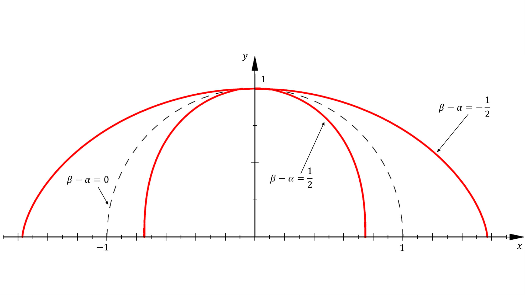 Figure 1
Peer Reviews
No public reviews on file for this paper yet. If you reviewed it on a platform where reviews are public (OpenReview, ICLR, NeurIPS, ICML), you can paste yours below so the community can read it here.
Videos
No videos yet. Explain this paper in a talk, walkthrough, or lecture? Add one.
11footnotetext: Università di Napoli Federico II, Dipartimento di Matematica e Applicazioni “R. Caccioppoli”, Complesso Monte S. Angelo, via Cintia, 80126 Napoli, Italy;
e-mail: [email protected], [email protected], [email protected], [email protected]: Department of Mathematics, Computational Foundry, College of Science, Swansea University, Bay Campus, Fabian Way, Swansea SA1 8EN, Wales, UK, e-mail: [email protected]
Some isoperimetric inequalities
with respect to monomial weights
A. Alvino1
,
F. Brock2
,
F. Chiacchio1
,
A. Mercaldo1
and
M.R. Posteraro1
Abstract.
We solve a class of isoperimetric problems on with respect to monomial weights. Let and be real numbers such that , . We show that, among all smooth sets in with fixed weighted measure , the weighted perimeter achieves its minimum for a smooth set which is symmetric w.r.t. to the –axis, and is explicitly given. Our results also imply an estimate of a weighted Cheeger constant and a lower bound for the first eigenvalue of a class of nonlinear problems.
Key words: isoperimetric inequality, weighted Cheeger set, eigenvalue problems
2000 Mathematics Subject Classification: 51M16, 46E35, 46E30, 35P15
1. Introduction
The last two decades have seen a growing interest in isoperimetric inequalities with respect to weights.
In most cases, volume and perimeter in those inequalities carried the same weight, because such a setting corresponds to manifolds with density. However, most research dealt with inequalities where both the volume functional and perimeter functional carry the same weight, see for instance [5], [7], [8], [11], [24], [14], [15], [16], [17], [20], [23], [32], [33], [36], [37], [38] and the references therein.
More recently, also problems with different weight functions for perimeter and volume were studied, see for example [2], [3], [4], [6], [22], [25], [26], [29], [34], [35], [40] and the references therein. However, there is only a sparse literature on situations where the isoperimetric sets are not radial, see [26], [19], [1].
In this paper we study the following isoperimetric problem:
Minimize among all smooth sets satisfying
or equivalently
[TABLE]
Our main result, proved in Section 2, is the following:
Theorem 1.1**.**
Assume that
[TABLE]
and
[TABLE]
Then problem (P) has a minimizer which is given by
[TABLE]
Moreover, we have
[TABLE]
where and denotes the Beta function. In particular,
[TABLE]
Remark 1.1**.**
(a) First observe that is the half-circle when . Therefore Theorem 1.1 includes the result obtained by Maderna and Salsa in [33] (see also [14], [10]).
(b) Let . It is elementary to verify that,
1. if then ,
2. if then ,
3. if then ; see Figure 1.
Theorem 1.1 also allows to obtain a Faber-Krahn - type inequality for the so-called weighted Cheeger constant, and in turn a lower bound for the first eigenvalue for a degenerate elliptic operators. For similar results see also [9], [12], [13], [18], [30], [39], [41].
2. Isoperimetric inequality in the upper half plane
Let . Throughout this paper, we assume that and
[TABLE]
If is measurable, we set
[TABLE]
Further, we define the weighted area of by
[TABLE]
and the weighted relative perimeter of as
[TABLE]
It is well-known that, if is an open, rectifiable set, then the following equality holds
[TABLE]
( denotes -dimensional Hausdorff-measure.)
Remark 2.1**.**
The following properties of the perimeter are well-known:
Let be measurable with and .
Then there exists a sequence of open, rectifiable sets with and
[TABLE]
Further, we have
[TABLE]
for any sequence of open, rectifiable sets satisfying .
We define the ratio
[TABLE]
Remark 2.2**.**
We have for every .
We study the following isoperimetric problem:
[TABLE]
Our first aim is to reduce the class of admissible sets in the isoperimetric problem (P).
Throughout our proofs let denote a generic constant which may vary from line but does not depend on the other parameters.
The first two Lemmata give necessary conditions for a minimizer to exist.
Lemma 2.1**.**
If , then
[TABLE]
and (P) has no minimizer.
Proof: Let , (). Then
[TABLE]
Hence
[TABLE]
and the assertion follows.
Lemma 2.2**.**
Assume . Further, let be a nonempty, open and rectifiable set, which is not simply connected. Then there exists a nonempty, open and rectifiable set which is simply connected, such that
[TABLE]
Proof: (i) First assume that is connected. Let be the unbounded component of and set . Then is simply connected with and , so that (2.9) follows.
(ii) Next, let , with mutually disjoint, nonempty, open, connected and rectifiable sets , (, ). We set . Let us assume that for every . Then we have, since ,
[TABLE]
a contradiction. Hence there exists a number with . Then, repeating the argument of part (i), with in place of , we again arrive at (2.9).
Lemma 2.3**.**
There holds
[TABLE]
but (P) has no open rectifiable minimizer.
Proof: With as in the proof of Lemma 2.1, we calculate and
[TABLE]
Let be open, rectifiable and simply connected. Then is a closed Jordan curve with counter-clockwise representation
[TABLE]
where , , , and on . Using Green’s Theorem we evaluate
[TABLE]
Equality in (2.12) can hold only if and on , that is, if is a single straight segment which is parallel to the -axis. But this is impossible. Hence we find that
[TABLE]
To show the assertion in the general case, we proceed similarly as in the proof of Lemma 2.2:
Assume first that is connected and define the sets and as in the last proof. Using (2.13), with in place of , we obtain
[TABLE]
Finally, let be open and rectifiable. Then , with mutually disjoint, connected sets , (). Then (2.14) yields
[TABLE]
Now the assertion follows from (2.15) and (2.11).
Lemma 2.4**.**
Let . Then (2.8) holds and (P) has no minimizer.
Proof: Let , (). Then we have for all ,
[TABLE]
This implies
[TABLE]
and the assertion follows.
Next we recall the definition of the Steiner symmetrization w.r.t. the -variable. If is measurable, we set
[TABLE]
where , are defined in (2.2) and
[TABLE]
Note that is a symmetric interval with .
Since the weight functions in the functionals and do not depend on , we have the following well-known properties, see [28], Proposition 3.
Lemma 2.5**.**
Let be measurable. Then
[TABLE]
For nonempty open sets with we set and
[TABLE]
Remark 2.3. Assume that is a bounded, open and rectifiable set with and . Then it has the following representation,
[TABLE]
Lemma 2.6**.**
Let be a nonempty, bounded, open and rectifiable set with . Then we have
[TABLE]
where is given by (2).
Proof: Assume first that is represented by (2) where
[TABLE]
Then we have for every ,
[TABLE]
Furthermore, there holds
[TABLE]
In the general case the assertions follow from these calculations by approximation with sets of the type given by (2), (2.24).
Lemma 2.7**.**
Assume that
[TABLE]
and let be a bounded, open and rectifiable set with , and . Then there exist positive numbers and which depend only on and such that
[TABLE]
Proof: By (2.22) and (2.23) we have
[TABLE]
It follows that
[TABLE]
Setting , we obtain from (2.28) and (2.30),
[TABLE]
which implies that
[TABLE]
with a constant which depends only on and . By (2.26) we have that
[TABLE]
Hence it follows that
[TABLE]
Using (2.31) and (2.32) this leads to (2.27).
Lemma 2.8**.**
Assume (2.25) and (2.26). Then problem (P) has a minimizer which is symmetric w.r.t. the -axis.
Proof: We proceed in steps.
Step 1: A minimizing sequence :
Let a minimizing sequence, that is, . In view of the Remarks 2.1 and 2.2 and the Lemmata 2.2 and 2.6 we may assume that is open, simply connected and rectifiable with , and , ().
Step 2: Parametrization of :
Denote . It is clear that a simple smooth curve with
[TABLE]
where denotes the usual arclength parameter, , , and for every , (). We orientate in such a way that the mapping is nonincreasing and . Setting and , we have by Lemma 2.6,
[TABLE]
where and do not depend on . Note that in case that . Further, Lemma 2.6, (2.23) shows that
[TABLE]
For our purposes it will be convenient to work with another parametrization of : We set
[TABLE]
Then , and we evaluate
[TABLE]
Step 3: Limit of the minimizing sequence :
Since , we obtain from (2.34) and (2.39) that the family is equibounded and uniformly Lipschitz continuous on . Hence there is a function with such that, up to a subsequence,
[TABLE]
Moreover, setting , , the bounds (2.27) are in place and is nonincreasing.
Let
[TABLE]
Then from (2.35) and (2.38) we obtain that the families and are equibounded on every closed subset of . Hence there exists a function which is locally Lipschitz continuous on , such that, up to a subsequence,
[TABLE]
Moreover, from (2.35) and (2.38) we find that
[TABLE]
Let be the set in with such that is represented by the pair of functions
[TABLE]
In view of (2.43) we have that
[TABLE]
Step 4: A minimizing set :
We prove that
[TABLE]
In order to prove the first equality, since , we prove that
[TABLE]
Fix some . Then (2.38), (2.39), (2.43), (2.40) and (2.41) yield
[TABLE]
Further, (2.38) and (2.43) give
[TABLE]
Now (2.48), (2.49), (2) and (2.44) yield (2.46) and therefore the first of the equalities in (2.45).
Now we prove the second inequality in (2.45). With as above we also have
[TABLE]
In view of (2.40) and (2.41) it follows that .
On the other hand, we have
[TABLE]
Define
[TABLE]
Letting we obtain
[TABLE]
Hence is a minimizing set.
Note that must be simply connected in view of Lemma 2.2, which implies that there is a number such that
[TABLE]
This finishes the proof of Lemma 2.8.
Next we obtain differential equations for the functions and in the proof in Lemma 2.8.
Lemma 2.9**.**
Assume (2.25) and (2.26). Then the minimizer obtained in Lemma 2.11 is bounded, and its boundary given parametrically by
[TABLE]
where the functions satisfy the following equations:
[TABLE]
together with the boundary conditions
[TABLE]
for some numbers and . Finally, the curve (2.9) is strictly convex.
Proof: We proceed in 4 steps.
Step 1: Euler equations :
After a rescaling the parameter , we see that the functions and in the previous proof annihilate the first variation of the functional
[TABLE]
under the constraint
[TABLE]
Hence and satisfy the Euler equations
[TABLE]
where is a Lagrangian multiplier, and
[TABLE]
In addition, the following boundary conditions are satisfied:
[TABLE]
Step 2: Boundedness:
It will be more convenient to rewrite the above conditions in terms of the arclength parameter : Set
[TABLE]
where . Then we have so that (2.57), (2.58) yield the system of equations (2.52), (2.53). Integrating (2.53) we obtain
[TABLE]
for some .
Assume first that is unbounded. Then , and in view of (2.42) we have that . If , then this would imply , which is impossible. Hence we may restrict ourselves to the case .
There is a sequence such that . Using in (2.63) and passing to the limit gives . Plugging this into (2.52), we find
[TABLE]
Multiplying (2.64) with and integrating, we obtain
[TABLE]
or equivalently,
[TABLE]
for some . Using in (2.65) and taking into account that , and , we arrive again at a contradiction. Hence is bounded, and we deduce the boundary conditions (2.55)-(2.9).
Step 3: is positive :
Multiplying (2.52) with and integrating from to gives
[TABLE]
Using integration by parts this yields
[TABLE]
The first two boundary terms in this identity vanish due to the boundary conditions (2.55)-(2.9) and the two integrals are positive since and . It follows that
[TABLE]
Now, considering equation (2.63) at and taking into account the boundary conditions (2.9), we find
[TABLE]
which implies that
[TABLE]
Step 4: Strict convexity :
From (2.52) and (2.53) we obtain
[TABLE]
Hence, using (2.63), we find for the curvature of the curve , (),
[TABLE]
The last expression is positive by (2.66) and (2.67), which means that is strictly convex. The Lemma is proved.
Lemma 2.10**.**
Assume (2.25) and (2.26), and let be given by (2.9)-(2.9). Then .
Proof: Supposing that , we will argue by contradiction. We proceed in 3 steps.
Step 1: Another parametrization of :
Let
[TABLE]
Since is strictly convex, there are functions such that
[TABLE]
Furthermore, the Euler equations (2.52), (2.53) lead to
[TABLE]
Using (2.71) and the fact that
[TABLE]
lead to
[TABLE]
Finally, the boundary conditions (2.70)–(2.72) lead to the following formulas:
[TABLE]
Step 2: Curvature:
In the following, we will refer to points as points of the ’lower curve’ and to points as points of the ’upper curve’, ().
The signed curvature (see (2)) can be expressed in terms of the functions and . More precisely, we have
[TABLE]
Accordingly, we will write
[TABLE]
Finally, let be taken such that and . Then formula (2.63) taken at leads to
[TABLE]
Plugging this into (2) we find
[TABLE]
Differentiating (2.83) we evaluate
[TABLE]
Since for , this in particular implies
[TABLE]
Step 4:
We claim that
[TABLE]
First observe that (2.86) immediately follows from (2.85) if . Thus it remains to consider the case
[TABLE]
From (2.84) and the fact that for we find that
[TABLE]
This means that
[TABLE]
for some (small) . Now assume that (2.86) does not hold. By (2.89) there exists a number such that
[TABLE]
We claim that (2.90) implies that
[TABLE]
To prove (2.92), observe first that
[TABLE]
Then, integrating (2.90) over leads to
[TABLE]
which implies (2.92). Now, from (2.92) we deduce
[TABLE]
Together with (2.77) and (2.78) we obtain from this
[TABLE]
or, equivalently
[TABLE]
Furthermore, multiplying (2.73) by , respectively (2.74) by , adding both equations and taking into account (2.91) leads to
[TABLE]
Using once more (2.77) and (2.78) then gives
[TABLE]
or equivalently,
[TABLE]
From this and (2.93) we then obtain
[TABLE]
Setting
[TABLE]
this leads to
[TABLE]
But this contradicts Lemma A (Appendix). This finishes the proof of (2.86).
Step 5:
Since , (2.86) implies that
[TABLE]
which contradicts the boundary conditions (2.72). Hence we must have that .
Now we are in a position to give a
Proof of Theorem 1.1: We split into two cases.
Case 1: Assume that
[TABLE]
By Lemma 2.10 we have . Now, since , equation (2.53) at yields
[TABLE]
so that
[TABLE]
In view of Remark 2.2 we may rescale in such a way that . Then (2.98) at gives . Since for , we have with a decreasing function . Writing
[TABLE]
we obtain
[TABLE]
and integrating this leads to (1.3) and (1.4).
Case (ii) Now assume that
[TABLE]
Since the case is trivial, we may assume . Let us fix such .
First observe that for every smooth domain , the mapping
[TABLE]
is continuous. Furthermore, from Case (i) we see that the mapping
[TABLE]
is continuous, and the limit
[TABLE]
exists.
Now let be the domain that is given by formulas (1.3), (1.4), with . Then we also have
[TABLE]
which implies that .
Assume that
[TABLE]
Then there is a smooth set such that also
[TABLE]
But by (2.101) this implies that
[TABLE]
when and is small, which is impossible. Hence we have that
[TABLE]
This finishes the proof of the Theorem.
Finally we evaluate . Put . With the Beta function and the function given by (1.4) we have
[TABLE]
and
[TABLE]
Using the identity
[TABLE]
we obtain
[TABLE]
which is (1.5). In case of this leads to
[TABLE]
Remark 2.3**.**
It is also well-known that the isoperimetric inequality is equivalent to the following functional inequality, (see [1], Lemma 3.5).
[TABLE]
3. Applications
In this section we firstly show that our isoperimetric inequality implies a sharp estimate of the so-called weighted Cheeger constant.
Then we deduce an estimate of the first eigenvalue to a degenerate elliptic Dirichlet boundary values problem. We begin by introducing some function spaces that will be used in the sequel.
Let be an open subset of and .
By we denote the weighted Hölder space of measurable functions such that
[TABLE]
Then let be the weighted Sobolev space of all functions possessing weak first partial derivatives which belong to . A norm in is given by
[TABLE]
For any function we write
[TABLE]
Then let be the weighted BV-space of all functions such that . A norm on is given by
[TABLE]
Let us explicitly remark that for an open bounded set the following equality holds
[TABLE]
Finally let be the set of all the functions that vanish in a neighborhood of . Then will denote the closure of in the norm of .
Finally we denote by the set , for , such that .
3.1. Weighted Cheeger sets
We define the weighted Cheeger constant of an open bounded set as
[TABLE]
We firstly prove that the existence of an admissible set which realizes the minimum in (3.1) (see also [41]).
Lemma 3.1**.**
Assume and . For any open bounded set , there exists at least one set , the so-called weighted Cheeger set, such that
[TABLE]
Proof: Since is open, is finite: Indeed, it is easy to verify that for any ball with , the ratio is finite.
Let be a minimizing sequence for (3.1). Since is bounded, we have
[TABLE]
Now fix . There exists an index such that
[TABLE]
Since is bounded, for all , we get
[TABLE]
This implies
[TABLE]
Hence is an equibounded family in weighted norm. Thus by Lemma B (Appendix), up to subsequences, converges in the weighted norm and pointwise a.e. to a function . Moreover there exists a subset such that .
Since is a minimizing sequence, by lower semicontinuity of perimeter and Lebesgue dominated convergence theorem, we get
[TABLE]
It remains to prove that is an admissible set, that is we need to prove that
[TABLE]
Assume by contradiction that . This implies that .
Now for a fixed consider the set
[TABLE]
Now the following inequality holds true
[TABLE]
where , if and for a suitable such that a ball of radius contains , if . Denote by a ball of radius having the same Lebesgue measure of . By the classical isoperimetric inequality, we get
[TABLE]
This yields a contradiction. Therefore (3.4) holds true and the conclusion follows.
Once we have proved the existence of a weighted Cheeger set, we can obtain the following result.
Theorem 3.1**.**
Assume and and , and let be a bounded open subset . Then the following estimate holds true
[TABLE]
Proof: Let be a nonempty subset of with . By our isoperimetric inequality Theorem 1.1 and since with , we have that
[TABLE]
It remains to prove the equality in (3.5). Let be a nonempty subset of . Then we have and
[TABLE]
for all . Since , there exists such that . Therefore
[TABLE]
which proves the equality in (3.5).
Remark 3.1. Theorem 3.1 could be stated as an estimate of the first eigenvalue of the weighted 1-laplacian.
3.2. A nonlinear eigenvalue problem
Let be a bounded domain and let We consider the following weighted eigenvalue problem
[TABLE]
where
[TABLE]
By a solution to problem (3.8) we mean a function such that
[TABLE]
for all function such that on
Let us denote by the range of values of and for which the isoperimetric inequality holds true. We have that
[TABLE]
if and only if
[TABLE]
Furthermore the smallest eigenvalue of problem (3.8), has the following variational characterization
[TABLE]
Indeed, see e.g. Theorem 8.9 in [27], for any the following compact embedding holds true
[TABLE]
By adapting the arguments used in [21], [31], we obtain the following result
Theorem 3.2**.**
Let then the following estimate holds true
[TABLE]
Remark 3.2. If and , a Faber-Krahn type inequality for holds true (see [33]). Indeed in this case, we have
Proof of Theorem 3.2 We claim that
[TABLE]
where is defined in (3.1). Let be an eigenfunction corresponding to . Hölder’s inequality gives
[TABLE]
and therefore
[TABLE]
If we set , then the previous inequality becomes
[TABLE]
On the other hand Coarea formula yields
[TABLE]
[TABLE]
[TABLE]
[TABLE]
The claim is hence proved. It immediately implies Theorem 3.2, thanks to (3.5).
4. Appendix
We prove two technical results.
Lemma A: Let with . Then
[TABLE]
Proof: We fix and define
[TABLE]
Then
[TABLE]
Hence which together with (4.3) and (4.4) implies that
[TABLE]
Furthermore we have
[TABLE]
Together with (4.2) and (4.4) this implies
[TABLE]
which is (4.1).
**Lemma B: **Let be a bounded sequence. Then there exists a subsequence that converges in and a.e. in to some function .
Proof: Put and let for any .
Let . By a classical compactness result in the unweighted case, there exists a function and an increasing sequence of integers such that
[TABLE]
By choosing to be a subsequence of , (), we can achieve that in , .
Now put
[TABLE]
In view of our isoperimetric inequality, the sequence is equibounded in . We have the following estimate:
[TABLE]
with constants that do not depend on . This implies that .
Let . Choose large enough such that
[TABLE]
and then large enough such that
[TABLE]
Then we obtain
[TABLE]
where does not depend on . From this the assertion follows.
**Acknowledgement: ** We are grateful to M. van den Berg for giving us useful suggestions. The first, third, fourth and fifth authors are members of the Gruppo Nazionale per l’Analisi Matematica, la Probabilità e le loro Applicazioni (GNAMPA) of the Istituto Nazionale di Alta Matematica (INdAM) and they thank this institution for the support. The second author was partially supported by Leverhulme Trust ref. VP1-2017-004. We are also grateful to the Departments of Mathematics of Swansea University and of the University of Naples Federico II, and to South China University of Technology (ISAM) at Guangzhou for visiting appointments and their colleagues for their kind hospitality.
The reference list from the paper itself. Each links out to its DOI / PubMed record.
- 1[1] E. Abreu, L.G. Fernandes , On existence and nonexistence of isoperimetric inequalities with different monomial weights. ar Xiv:1904.01441 v 2, 11 Apr 2019.
- 2[2] A. Alvino, F. Brock, F. Chiacchio, A. Mercaldo, M.R. Posteraro , Some isoperimetric inequalities on ℝ N superscript ℝ 𝑁 \mathbb{R}^{N} with respect to weights | x | α superscript 𝑥 𝛼 |x|^{\alpha} , J. Math. Anal. Appl. 451 , no. 1, (2017), 280–318.
- 3[3] A. Alvino, F. Brock, F. Chiacchio, A. Mercaldo, M.R. Posteraro , On weighted isoperimetric inequalities with non-radial densities (2018), Appl. Anal. , to appear doi.org/10.1080/00036811.2018.1506106
- 4[4] A. Alvino, F. Brock, F. Chiacchio, A. Mercaldo, M.R. Posteraro , The isoperimetric problem for a class of non-radial weights and applications (2018), J. Differential Equations, to appear.
- 5[5] V. Bayle, A. Cañete, F. Morgan, C. Rosales , On the isoperimetric problem in Euclidean space with density. Calc. Var. PDE 31 (2008), 27–46.
- 6[6] M.F. Betta, F. Brock, A. Mercaldo, M.R. Posteraro , A weighted isoperimetric inequality and applications to symmetrization. J. Inequal. Appl. 4 (1999), no. 3, 215–-240.
- 7[7] M.F. Betta, F. Brock, A. Mercaldo, M.R. Posteraro , Weighted isoperimetric inequalities on ℝ N superscript ℝ 𝑁 \mathbb{R}^{N} and applications to rearrangements. Math. Nachr. 281 (2008), no. 4, 466–498.
- 8[8] W. Boyer, B. Brown, G. Chambers, A. Loving, S. Tammen , Isoperimetric regions in ℝ n superscript ℝ 𝑛 \mathbb{R}^{n} with density r p superscript 𝑟 𝑝 r^{p} , Anal. Geom. Metr. Spaces 4 (2016), 236–265.