Enhanced interaction effects in the vicinity of the topological transition
C. C. A. Houghton, E. G. Mishchenko, and M. E. Raikh

TL;DR
This paper investigates how electron interactions near a topological transition significantly affect quasiparticle properties, spectrum renormalization, and electron density oscillations, leading to observable effects on conductivity.
Contribution
It provides a detailed analysis of interaction effects on electrons near a topological transition, highlighting spectrum renormalization and anisotropic Friedel oscillations.
Findings
Electrons near the transition have short inelastic lifetimes.
Interactions cause strong spectrum renormalization near the transition.
Friedel oscillations become anisotropic and influence conductivity.
Abstract
A metal near the topological transition can be loosely viewed as consisting of two groups of electrons. First group are "bulk" electrons occupying most of the Brillouin zone. Second group are electrons with wave vectors close to the topological transition point. Kinetic energy, , of electrons of the first group is much bigger than kinetic energy, , of electrons of the second group. With electrons of the second group being slow, the interaction effects are more pronounced for these electrons. We perform a calculation illustrating that electrons of the second group are responsible for inelastic lifetime making it anomalously short, so that the concept of quasiparticles applies to these electrons only marginally. We also demonstrate that interactions renormalize the spectrum of electrons in the vicinity of topological transition, the parameters of renormalized spectrum…
Click any figure to enlarge with its caption.
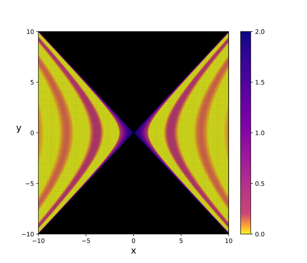 Figure 1
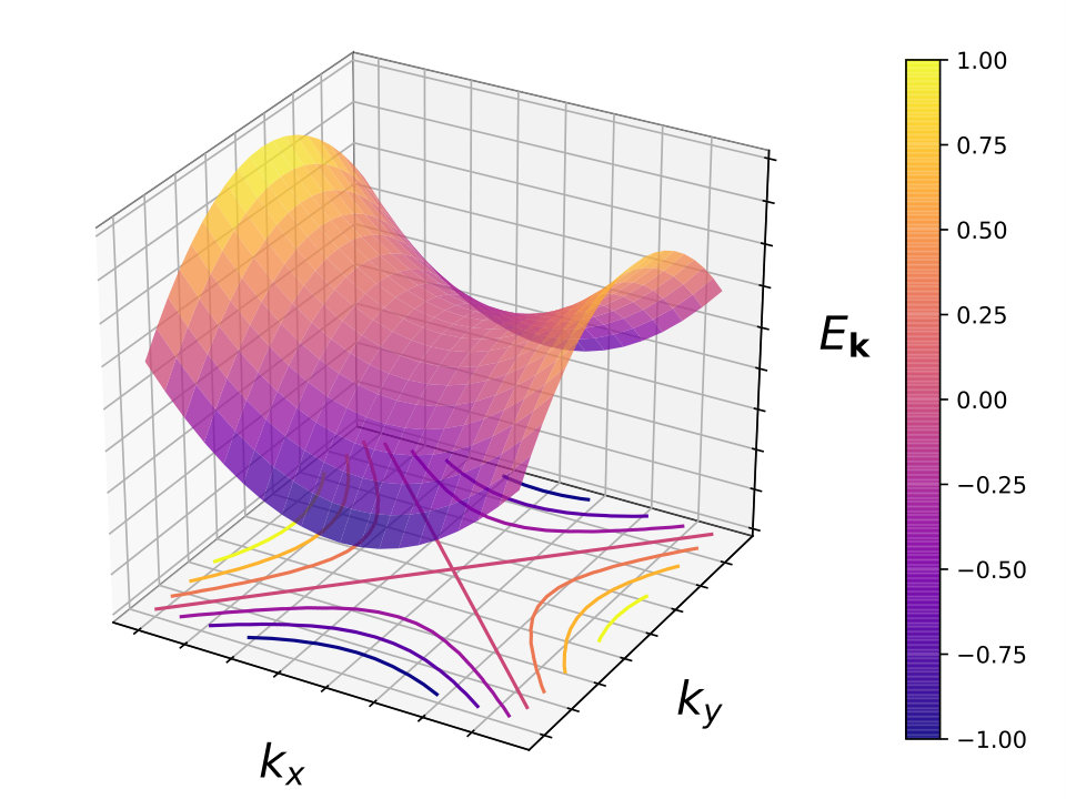 Figure 2
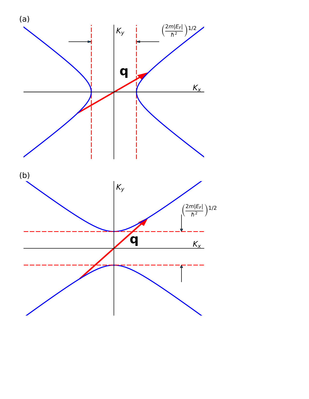 Figure 3
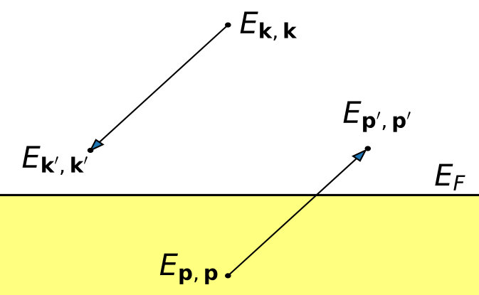 Figure 4
Peer Reviews
No public reviews on file for this paper yet. If you reviewed it on a platform where reviews are public (OpenReview, ICLR, NeurIPS, ICML), you can paste yours below so the community can read it here.
Videos
No videos yet. Explain this paper in a talk, walkthrough, or lecture? Add one.
Enhanced interaction effects in the vicinity of the topological transition
C. C. A. Houghton, E. G. Mishchenko, and M. E. Raikh
Department of Physics and Astronomy, University of Utah, Salt Lake City, UT 84112
Abstract
A metal near the topological transition can be loosely viewed as consisting of two groups of electrons. First group are “bulk” electrons occupying most of the Brillouin zone. Second group are electrons with wave vectors close to the topological transition point. Kinetic energy, , of electrons of the first group is much bigger than kinetic energy, , of electrons of the second group. With electrons of the second group being slow, the interaction effects are more pronounced for these electrons. We perform a calculation illustrating that electrons of the second group are responsible for inelastic lifetime making it anomalously short, so that the concept of quasiparticles applies to these electrons only marginally. We also demonstrate that interactions renormalize the spectrum of electrons in the vicinity of topological transition, the parameters of renormalized spectrum being strongly dependent on the proximity to the transition. Another many-body effect that evolves dramatically as the Fermi level is swept through the transition is the Friedel oscillations of the electron density created by electrons of the second group around an impurity. These oscillations are strongly anisotropic with a period depending on the direction. Scattering of electrons off these oscillations give rise to a temperature-dependent ballistic correction to the conductivity.
I Introduction
Topological transitions in metals take place when, upon the change of a certain external parameter, the connectivity of the Fermi surface undergoes a transformation. The concept of topological transition was introduced by I. M. Lifshitz in 1960.Lifshitz1960 . Lifshitz demonstrated that thermodynamic characteristics of a metal exhibit a singular behavior in the vicinity of the transition. Such a singular behavior was subsequently observed experimentally Experiment1983 ; Experiment1984 . First experiments were conducted on 3D metallic alloysExperiment1983 and 2D semiconductor superlattices.Experiment1984 In the past decade the class of materials in which the signatures of the topological transitions were uncovered has significantly broadened1 ; 2 ; 3 ; 4 ; 5 ; 6 ; 7 ; 8 to include heavy fermions, graphite, germanene, cilicene, ruthinades, etc.
On the theoretical side, kinetic and thermodynamic characteristics of metals near the topological transitionsVarlamov1985 ; Varlamov1986 ; Blanter1990 ; Blanter1991 ; Ablyazov1991 ; Golosov1991 ; Mobius were actively studied after the experiments.Experiment1983 ; Experiment1984 The results are reviewed in Ref. VarlamovReview, . On the conceptual level, the main theoretical finding is that, in addition to the single-particle density of states, the transition manifests itself in the energy dependence of the impurity scattering time of carriers, which, at the same time, broaden the transition. Recent theoretical interest to the topological transitionsWeyl ; Thorus ; Chi-Ken2016 ; Graphene ; Volovik ; Galperin is mostly motivated by the invent of new materials with strong spin-orbit coupling.
The role played by electron-electron interactions in the topological transition was considered in Ref. Mobius, with a general conclusion that, away from Pomeranchuk instability, Fermi-liquid effects renormalize the singular part of thermodynamic quantities.
The goal of the present paper is to trace how the standard many-body effects for an isotropic spectrum get modified in the vicinity of the topological transition. We will consider the following effects: Friedel oscillations of the electron density, interaction-induced modification of the electron spectrum, and the interaction-induced electron lifetime caused by the creation of the electron-hole pairs. We find that the proximity to the transition gives rise to additional Friedel oscillations with very long period, which are strongly anisotropic and get rotated by as the Fermi level is swept through the transition.
Our main finding is that electron lifetime, , associated with creation of pairs, shortens dramatically in the vicinity of the transition. Directly at the transition, we have , so that the concept of the Fermi liquid applies only marginally.
Since the interaction effects are more pronounced in two dimensions, we will choose the simplest form of the spectrum in the vicinity of the topological transition
[TABLE]
see Fig. 1. The transition corresponds to the position of the Fermi level . As changes from negative to positive, the Fermi surface near evolves as illustrated in Fig. 2. Most importantly, the typical wave vector, , in the vicinity of the transition is small, while everywhere else in the Brillouin zone this wave vector is big, namely it is of the order of , where is the Fermi level measured from the bottom of the band.
While within a single-particle approach the topological transition causes a singular correction to the electron characteristics, interaction effects give rise to new distinct features, in particular, new Friedel oscillations and a new channel of inelastic relaxation.
II Friedel oscillations
For a parabolic spectrum, , the Friedel oscillations of the electron density, , created by a defect, are isotropic
[TABLE]
where is the Fermi wave vector.
Below we generalize the derivation of to the case of a hyperbolic spectrum Eq. (1) and demonstrate that it assumes the form
[TABLE]
Outside the quadrants the correction falls off exponentially at large .
On the opposite side of the transition, , the result Eq. (3) transforms into
[TABLE]
with . Therefore, the crossing from positive to negative is accompanied by rotation of the Friedel oscillations pattern by . At finite temperature, , the oscillations are cut off at distance such that , so that in the transition region the oscillations effectively disappear.
II.1 Derivation
Consider a short-range impurity with potential . It creates the following correction to the free-electron wave functions,
[TABLE]
Then the electron density,
[TABLE]
acquires the following correction
[TABLE]
where , and is a step-function. It is convenient to rewrite Eq. (7) in the form
[TABLE]
where we have introduced an auxiliary function
[TABLE]
To establish the analytical form of we switch to the new variables
[TABLE]
where is the azimuthal angle of . Then Eq. (9) takes the form
[TABLE]
Note that is present only in the argument of the -function. To perform the integration over we factorize this argument
[TABLE]
Now the integration over is straightforward and yields
[TABLE]
The upper limit in the integral Eq. (13) is infinity. The lower limit depends on the sign of . When the sign is negative, there is no pole in the denominator. Then the lower limit is zero and the integral reduces to the Macdonald function. For positive the lower limit is . The integral then reduces to the Bessel function of the second kind. Combining both cases, we write
[TABLE]
where . In the case of a parabolic spectrum the function is simply the Bessel function .
Now the expression for should be substituted into Eq. (8). Similarly to the parabolic spectrum, one has to use the large-argument asymptote of . We see that for the Macdonald function decays exponentially, so that there are no oscillations in two quadrants . For quadrants the long-distance asymptote of is , and differs by a phase from the asymptote, , of . Thus, the product contains in the same way as the product only with opposite sign. This allows to proceed directly to the result for
[TABLE]
Eq. (14) illustrates the general connectionBenaReview between the Friedel oscillations and the underlying spectrum.
III Spectrum renormalization
We start from the textbook expressionMahan for the exchange self-energy
[TABLE]
where is the Fermi distribution and is the Fourier component of the electron-electron interaction. We first assume that and choose for the screened Coulomb potential
[TABLE]
where is a bare dielectric constant and is the inverse screening radius which we will determine later.
Obviously, the integral over diverges at large leading to a general energy shift independent of . To calculate the spectrum renormalization we subtract this shift and get
[TABLE]
Now the integral Eq. (17) converges at . We are interested in the spectrum renormalization in the vicinity of the transition. Assuming that , we expand the integrand in parameter . This yields
[TABLE]
The expansion in Eq. (18) is carried out to the second order in , since the first-order term vanishes upon the angular integration. Indeed, this term changes sign upon replacement , where is the polar angle of the vector . On the other hand, the argument of contains , and it does not change upon this replacement. Thus the integration of the linear term over yields zero. The second and the third terms in Eq. (18) give rise to the following -correction to the spectrum
[TABLE]
It is instructive to rewrite this correction in the form
[TABLE]
We expect that interactions preserve the structure of the spectrum, . On the other hand, the first term in the numerator of Eq. (20) leads to the isotropic -correction. But it is easy to check that the condition
[TABLE]
is met, so that the coefficient in front of -term is zero. Final result for the spectrum renormalization reads
[TABLE]
For our choice the integrals over and over get decoupled. The first integral is equal to , while the second integral is equal to . It is convenient to cast Eq. (22) into the form of the renormalized mass in the spectrum Eq. (1)
[TABLE]
At finite , away from the transition, the dependence on comes from the integral over in Eq. (22). However, the leading dependence on originates from the parameter . Within the random-phase approximation the expression for the inverse screening radius reads
[TABLE]
where is the density of states at the Fermi level. In fact, diverges in the limit . Indeed, on has
[TABLE]
Substituting Eq. (25) into Eq. (24), we arrive to the following expression for renormalized mass
[TABLE]
IV Polarization Operator
Polarization operator for 2D electron gas with a parabolic spectrum was calculated for the first time by F. Stern.Stern1967 Below we calculate polarization operator for a hyperbolic spectrum Eq. (1). We start from the definition
[TABLE]
As a first step, we cast Eq. (27) into the form
[TABLE]
Introducing, similarly to Eq. (II.1), the new variables
[TABLE]
and replacing the sum by the integral, we obtain
[TABLE]
Note that the argument of the -function has the same form as the argument of the -function in Eq. (12) with instead of . Then the integration over is straightforward
[TABLE]
where the first square bracket is the result of integration over , and in the second square bracket we have isolated the parts even in .
It is convenient to rewrite Eq. (31) as follows
[TABLE]
where the parameters , , and are defined as
[TABLE]
Now the integration in Eq. (32) can be performed explicitly. The main contribution to the polarization operator comes from log-divergence of the integral at large . This divergence is cut off at . The and -dependencies are given by the sub-leading terms
[TABLE]
where the function is defined as
[TABLE]
The upper limit in the integral Eq. (35) is infinity. The lower limit is for positive and for negative . Correspondingly, the form of is different for and . Namely,
[TABLE]
It is easy to see that falls off as at large positive and as at large negative .
IV.1 Frequency domain
Note that the coefficient in front of leading logarithmic term does not depend on frequency. In 2D electron gas with parabolic spectrumStern1967 the analog of the combinations in Eq. (34) has the form \Big{[}\left(\hbar\omega-\frac{\hbar^{2}q^{2}}{2m}\right)^{2}-2\frac{\hbar^{2}q^{2}{\tilde{E}}{\scriptscriptstyle F}}{m}\Big{]}^{1/2}. At small , the polarization operator acquires an imaginary part, which is responsible for the ac conductivity, when . The corresponding condition for the hyperbolic spectrum reads . Firstly, since , the Fermi energy in the “bulk”, is much bigger than , we conclude that the ac response at low frequencies is dominated by the proximity to the topological transition. Secondly, this response is strongly anisotropic.
IV.2 Momentum domain
In the static limit, , the polarization operator is a universal function of the dimensionless momentum
[TABLE]
This function has a form
[TABLE]
for . Near the Kohn anomaly the behavior of is singular, . It gives rise to the long-period Friedel oscillations Eq. (14).
For the expression for polarization operator reads
[TABLE]
As a function of , the behavior of is linear. Note that the behaviors Eqs. (37), (38) differ from the static polarization operator for the isotropic spectrumStern1967 , where is constant for , while the Kohn anomaly, , is located to the right from .
To summarize, we have evaluated polarization operator in the entire domain of frequencies and momenta. In the static limit and for our result agrees with Ref. Chi-Ken2016, . While for parabolic spectrum, , the Kohn anomaly corresponds to the condition , the corresponding condition for the hyperbolic spectrum Eq. (1) reads
[TABLE]
This condition is illustrated in Fig. 2.
V Electron lifetime
The process which is responsible for a finite lifetime, , of an electron with energy, , above the Fermi level is creation of an electron-hole pair. Accurate calculation of for an electron gas with a quadratic spectrum was reported in Refs. time1, , time2, . The result reads
[TABLE]
The -dependence originates from the energy conservation, namely: , where is the energy of the secondary electron, while and are the energies of particles constituting an excited pair. The factor originates from the momentum conservation. To generalize Eq. (40) to the case of hyperbolic spectrum, we start from the golden-rule expression for the rate
[TABLE]
To perform the averaging over the directions of momenta, we introduce auxiliary variables , , and and invoke the integral representation of the -function
[TABLE]
Now the integration over momenta decouples into three integrals of the type . For a quadratic spectrum, this integral is expressed through a zero-order Bessel function, . Then the integral over in Eq. (42) assumes the form
[TABLE]
The angular-averaged is equal to . The magnitudes of all momenta in Eq. (43) are close to the Fermi momentum, . The long-distance behavior of the product of the four Bessel functions is . Then the integration over gives rise to the logarithm in Eq. (41), while generates in the denominator.
For a hyperbolic spectrum, the integral is given by the function defined by Eq. (9). Then, in place of integral Eq. (43), one has
[TABLE]
Depending on the polar angle of , the function either oscillates with (in the domain ) or decays with (in the domain ). In the first domain, with energies , , close to and wave vector close to , the slow part of the integrand in Eq. (44) reproduces, within a numerical factor, the result Eq. (40) for the hyperbolic spectrum.
Naturally, the applicability of Eq. (40) requires that . In the vicinity of the topological transition is small and the estimate for the lifetime follows from Eq. (40) upon setting . We conclude that, in the vicinity of the topological transition, .
Assume now that the Fermi level is . The question of interest is how depends on the direction, , of the momentum of the initial electron. For , energy conservation requires that, when the energy is positive, the energy is negative while the energy is positive, see Fig. 4. Then Eq. (44) assumes the form
[TABLE]
where is the magnitude of momentum of initial electron, and are momenta of the secondary electrons, and is the momentum of a hole.
To find the dependence of on we introduce instead of a new variable and obtain
[TABLE]
The form Eq. (46) suggests that the main contribution to the integral comes from the vicinity of . For these the exponent in the integrand rapidly oscillates with . The exceptions are the vicinities of when turns to zero when is close to .
As an example, consider a situation and set , with . The exponent in Eq. (46) does not oscillate for , where . Then the angular integration in Eq. (46) yields
[TABLE]
The above result suggests that the lifetime, , shortens dramatically for certain directions of momentum of an electron. Physical explanation of such a shortening is that the cost of creation of a pair by electron with these directions of momentum is anomalously low.
VI Concluding Remarks
(i) Ballistic correction to the conductivityGold1986 ; Zala ; Adamov , , of a 2D electron gas has the form , where is the interaction parameter.Zala The origin of this correction is electron scattering from the potential created by Friedel oscillations surrounding individual impurities. The amplitude of this process is sharply peaked at the scattering angle . For this angle, the momentum transfer is close to , the wave vector of the Friedel oscillation. For the hyperbolic spectrum, while the wave vector of the Friedel oscillations depends on the direction, but the mechanism of Refs. Gold1986, , Zala, still applies. It gets modified as illustrated in Fig. 2. Backscattering takes place between disjoint parts of the Fermi surface. Smallness of makes the ballistic correction progressively pronounced in the vicinity of the transition.
(ii) While calculating the spectrum renormalization we assumed that the form of interaction is screened Coulomb, see Eq. (16). In fact, the static polarization operator Eq. (37) contains a sub-leading term, describing the Kohn anomaly. This term is strongly anisotropic. An interesting question is how this anisotropy affects the spectrum renormalization. Denote with the correction to the inverse screening radius, describing the Kohn anomaly, . Expanding the interaction with respect to , we get
[TABLE]
This correction to gives rise to the following correction to the self-energy
[TABLE]
At small momenta, , Eq. (49) leads to the following contribution to the spectrum renormalization
[TABLE]
This correction diverges, the divergence comes from the vicinity of .
(iii) Divergence of lifetime for directions of momenta close to also hints at strong renormalization of the spectrum for these momenta.
(iv) With regard to observables, interaction-induced modification of the effective mass manifests itself in the magneto-oscillations. Behavior of magneto-oscillations in the vicinity of the topological transition constitutes a subfield called the magnetic breakdown, see e.g. the review Ref. breakdown, . As the Fermi level is swept through the topological transition, the period of magneto-oscillations doubles. The width of the domain of where this doubling takes place is , where is the magnetic length. For the coupling of the semiclassical trajectories is determined by tunneling under the magnetic barrier.barrier Then the dependence of the effective mass on affects the barrier transmission.
Electron lifetime is measured in 2D-2D tunneling experiments.Tunnel1 ; Tunnel2 The lifetime defines the width of the peak in the tunnel conductance measured versus the dc bias applied between the layers.
(v) There is a conceptual similarity between Friedel oscillations of elections of the electron density created by an impurity and the oscillations of the spin density created by a magnetic impurityRoth1966 . In this regard, long-period Friedel oscillations in the vicinity of the topological transition are similar to the long-period behavior of the RKKY interaction established in Ref. Golosov1991, .
VII Acknowledgements
The work was supported by the Department of Energy, Office of Basic Energy Sciences, Grant No. DE-FG02-06ER46313.
The reference list from the paper itself. Each links out to its DOI / PubMed record.
- 1(1) I. M. Lifshitz, “Anomalies of electron characteristics of a metal in the high pressure region,” Sov. Phys. JETP 11 , 1130 (1960).
- 2(2) V. S. Egorov and A. N. Fedorov, “Thermopower of lithium-magnesium alloys at the 2 1 / 2 2 1 2 2~{}1/2 -order transition,” Sov. Phys. JETP 58 , 959 (1983).
- 3(3) N. V. Zavaritskii and I. M. Suslov, “Structural features in the thermopower of a two-dimensional electron gas near topological transitions,” Sov. Phys. JETP 60 , 1243 (1984).
- 4(4) E. A. Yelland, J. M. Barraclough, W. Wang, K. V. Kamenev, and A. D. Huxley, “High-field superconductivity at an electronic topological transition in U Rh Ge,” Nat. Phys. 7 , 890 (2011).
- 5(5) M. Orlita, P. Neugebauer, C. Faugeras, A. L. Barra, M. Potemski, F. M. D. Pellegrino, and D. M. Basko, “Cyclotron Motion in the Vicinity of a Lifshitz Transition in Graphite,” Phys. Rev. Lett. 108 , 017602 (2012).
- 6(6) A. Varleta, M. Mucha-Kruczyński, D. Bischoff, P. Simonet, T. Taniguchi, K. Watanabe, V. Fal’ko, T. Ihn, and K. Ensslin, “Tunable Fermi surface topology and Lifshitz transition in bilayer graphene,” Synthetic Metals 210 , 19 (2015).
- 7(7) H.-R. Chang, J. Zhou, H. Zhang, and Y. Yao, “Probing the topological phase transition via density oscillations in silicene and germanene,” Phys. Rev. B 89 , 201411(R) (2015).
- 8(8) H. Chi, C. Zhang, G. Gu, D. E Kharzeev, Xi Dai, and Qiang Li, “Lifshitz transition mediated electronic transport anomaly in bulk Zr Te 5 ,” New J. Phys. 19 , 015005 (2017).