Measurement of the top quark Yukawa coupling from $\mathrm{t\bar{t}}$ kinematic distributions in the lepton+jets final state in proton-proton collisions at $\sqrt{s} =$ 13 TeV
CMS Collaboration

TL;DR
This paper measures the top quark Yukawa coupling by analyzing kinematic distributions in top-antitop events at 13 TeV, introducing a novel reconstruction technique to improve sensitivity, and finds the coupling consistent with the Standard Model within uncertainties.
Contribution
The study introduces a new method for reconstructing the top-antitop system with missing jets, enhancing measurement precision of the Yukawa coupling from LHC data.
Findings
Measured top quark Yukawa coupling ratio: 1.07^{+0.34}_{-0.43}
Upper limit of 1.67 at 95% confidence level
Consistent with Standard Model predictions within uncertainties
Abstract
Results are presented for an extraction of the top quark Yukawa coupling from top quark-antiquark () kinematic distributions in the lepton plus jets final state in proton-proton collisions, based on data collected by the CMS experiment at the LHC at 13 TeV, corresponding to an integrated luminosity of 35.8 fb. Corrections from weak boson exchange, including Higgs bosons, between the top quarks can produce large distortions of differential distributions near the energy threshold of production. Therefore, precise measurements of these distributions are sensitive to the Yukawa coupling. Top quark events are reconstructed with at least three jets in the final state, and a novel technique is introduced to reconstruct the system for events with one missing jet. This technique enhances the experimental sensitivity…
Click any figure to enlarge with its caption.
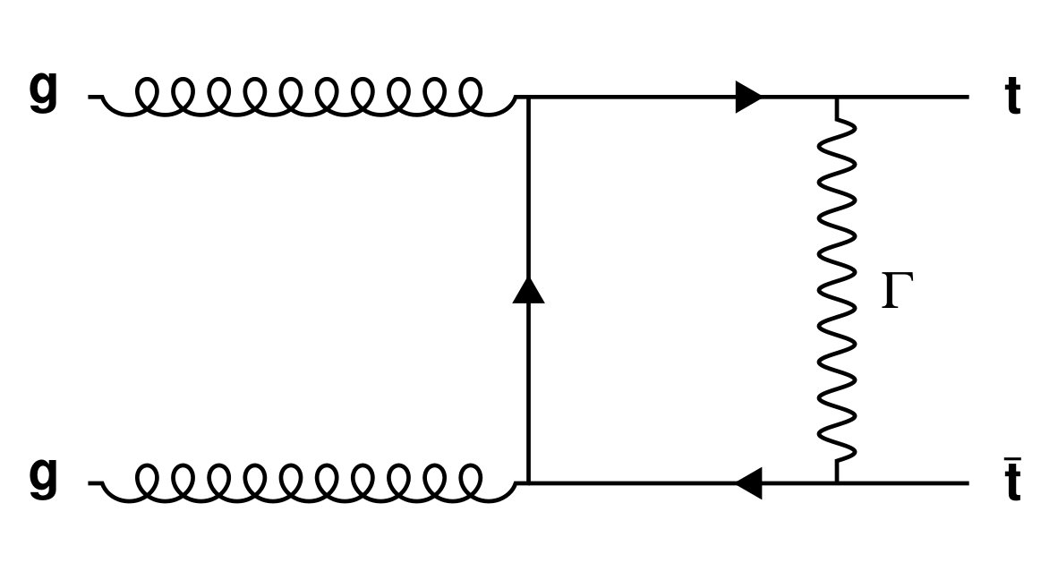 Figure 1
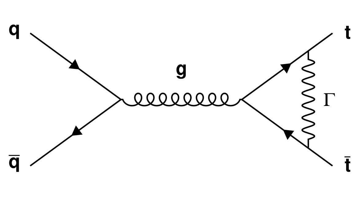 Figure 1
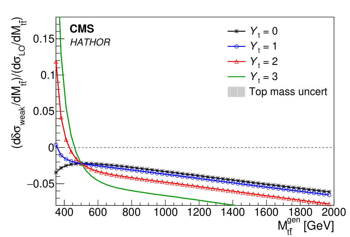 Figure 2
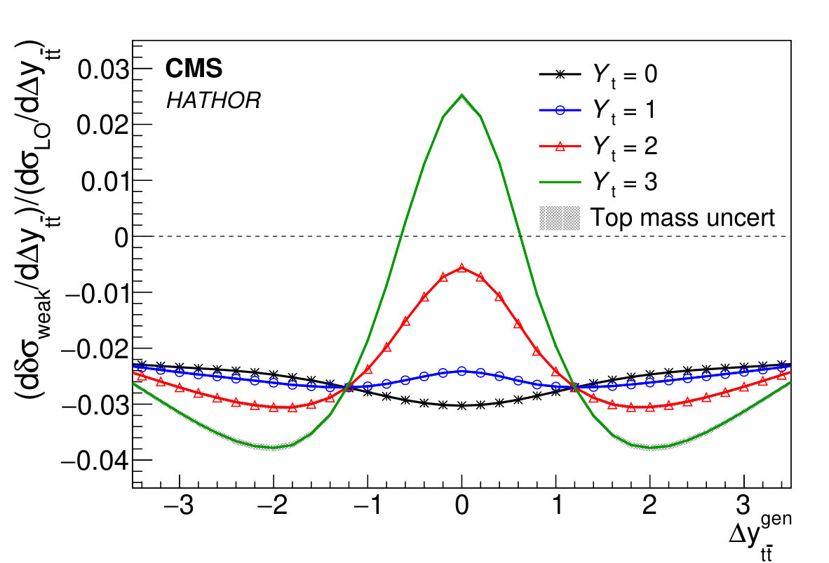 Figure 2
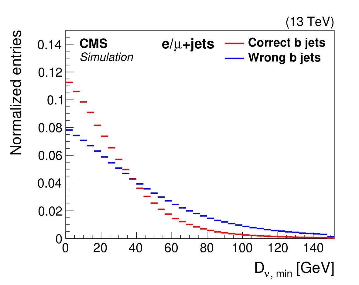 Figure 3
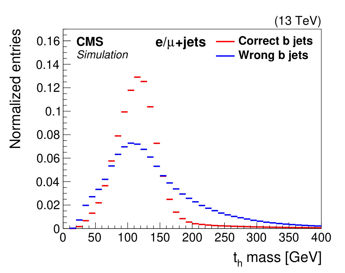 Figure 3
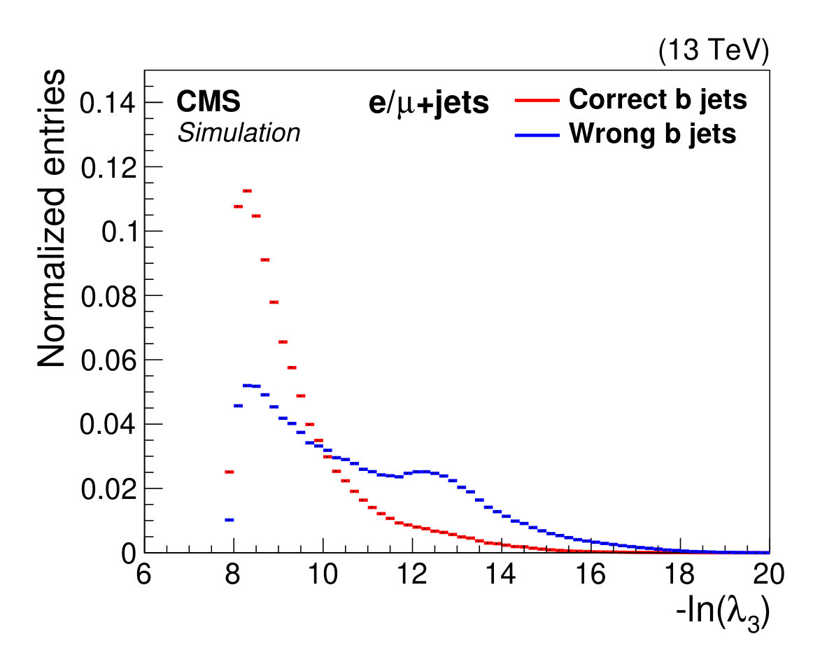 Figure 3
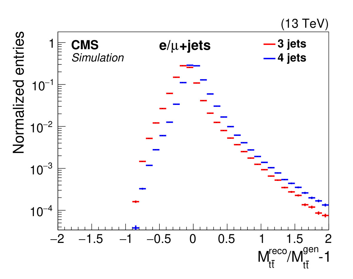 Figure 4
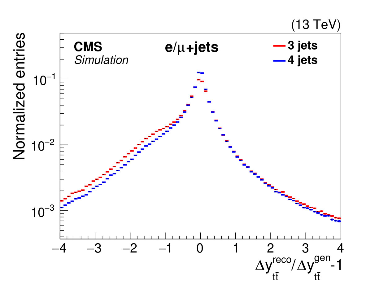 Figure 4
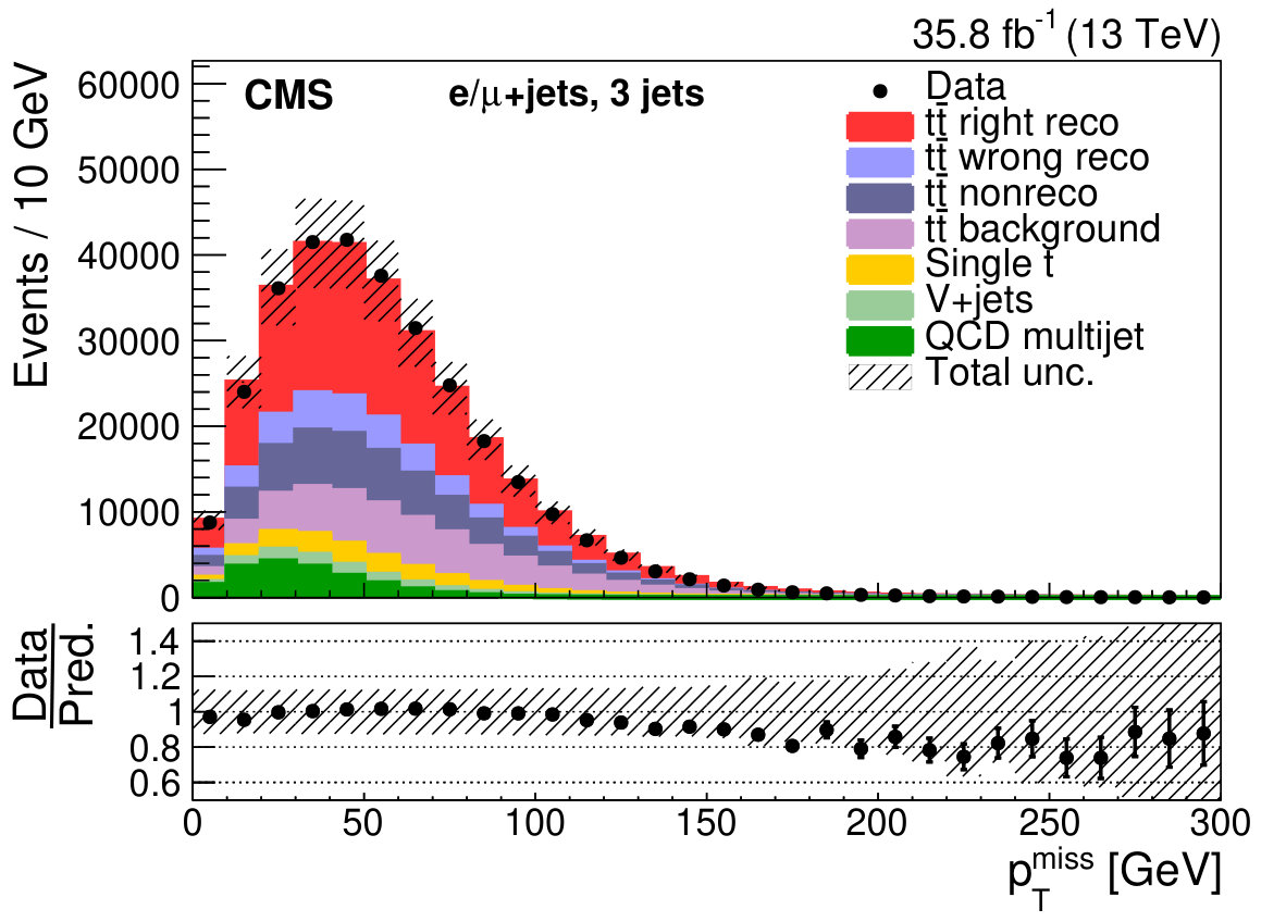 Figure 5
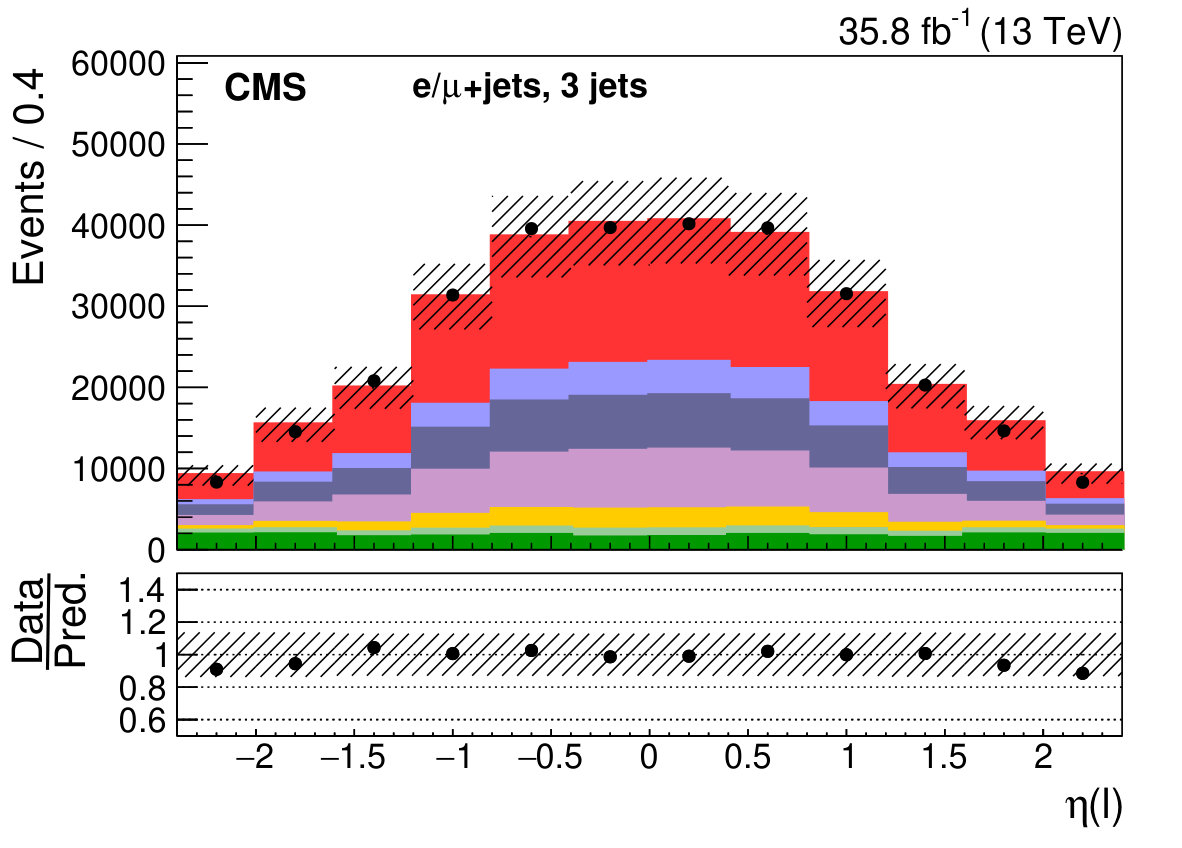 Figure 5
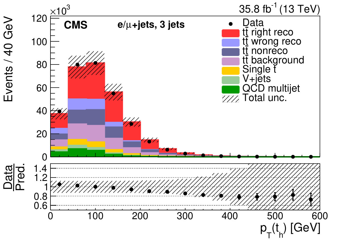 Figure 5
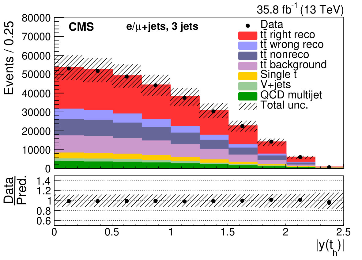 Figure 5
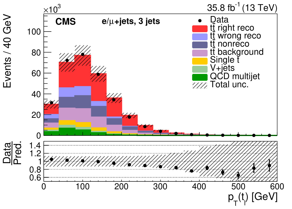 Figure 5
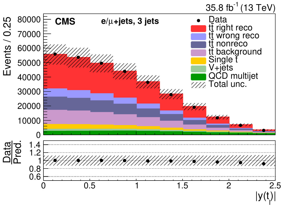 Figure 5
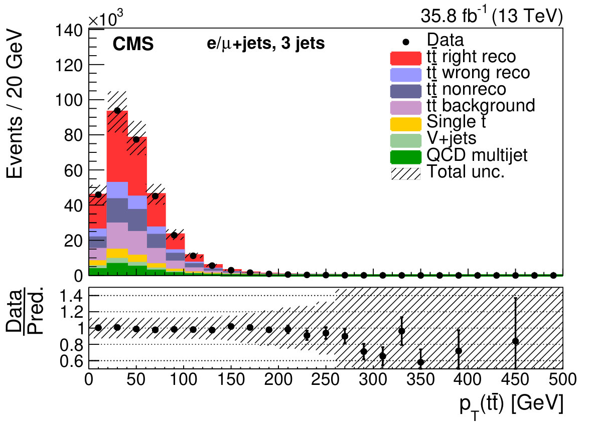 Figure 5
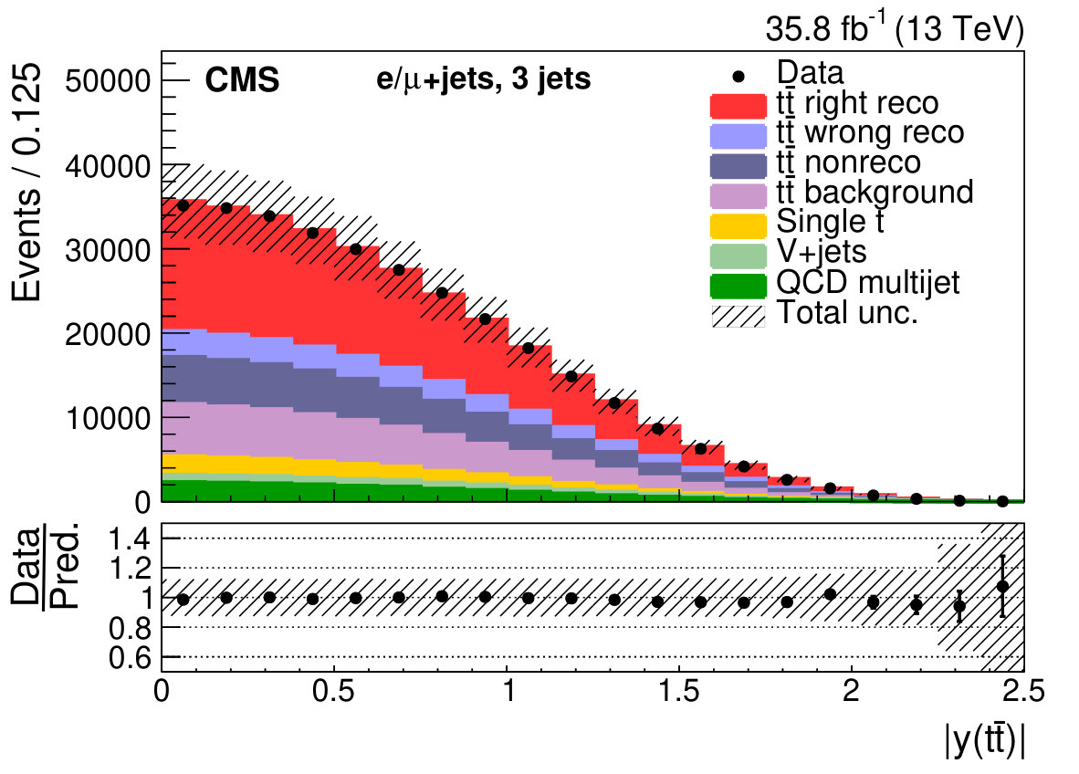 Figure 5
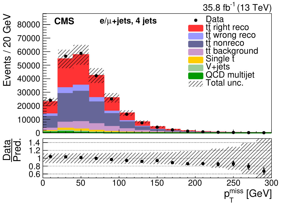 Figure 6
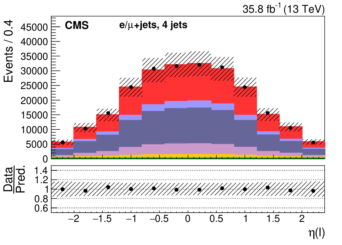 Figure 6
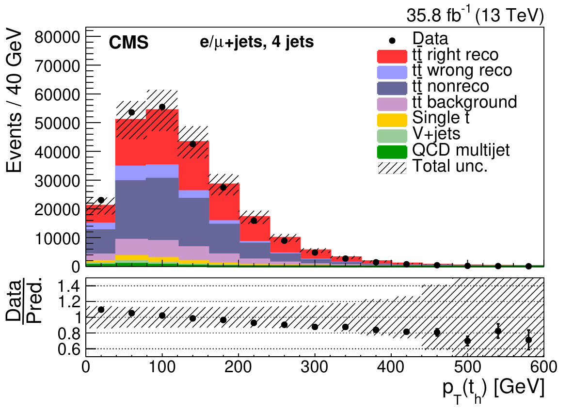 Figure 6
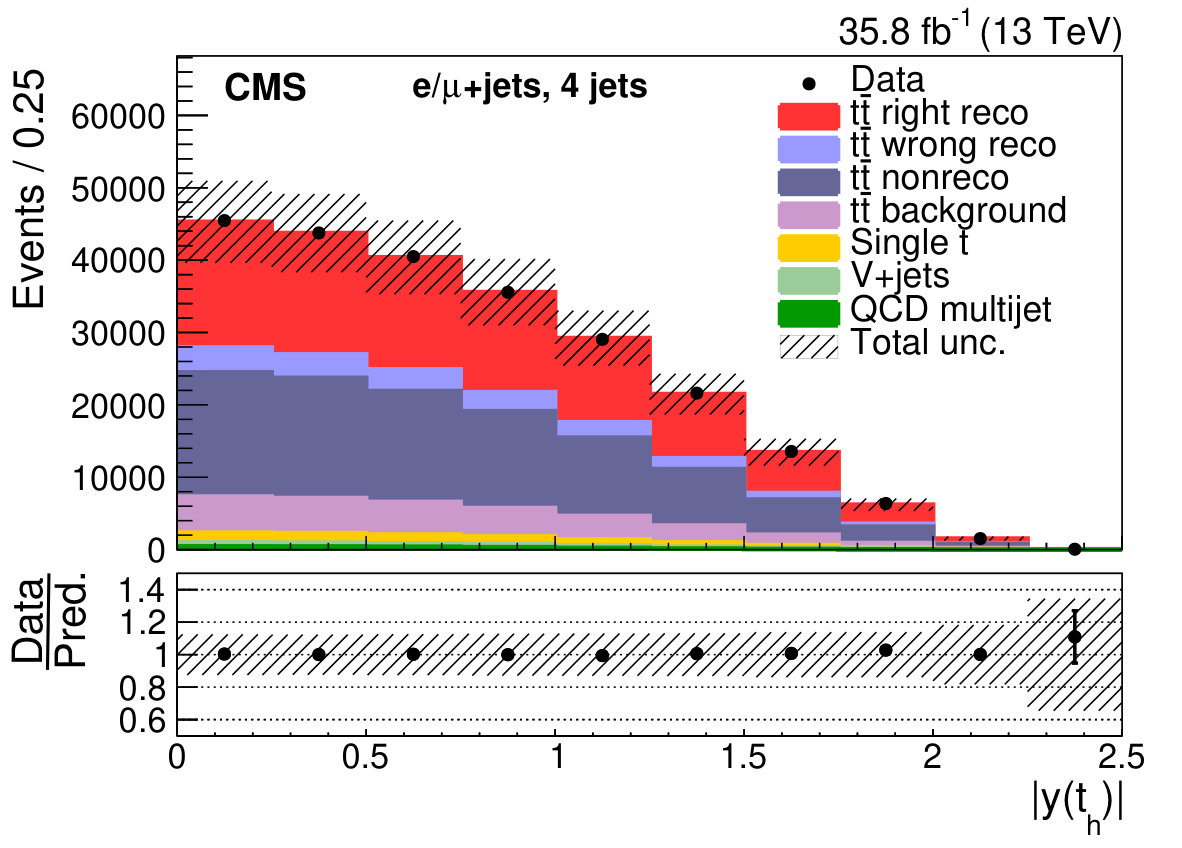 Figure 6
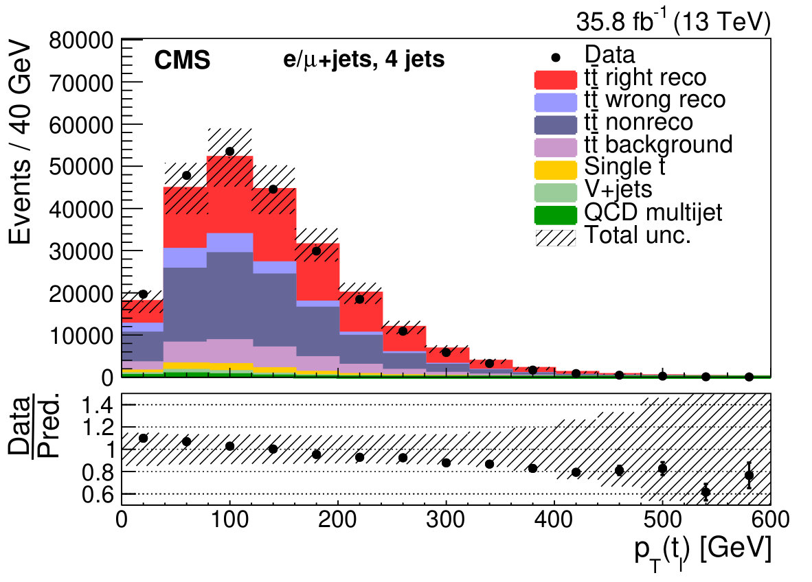 Figure 6
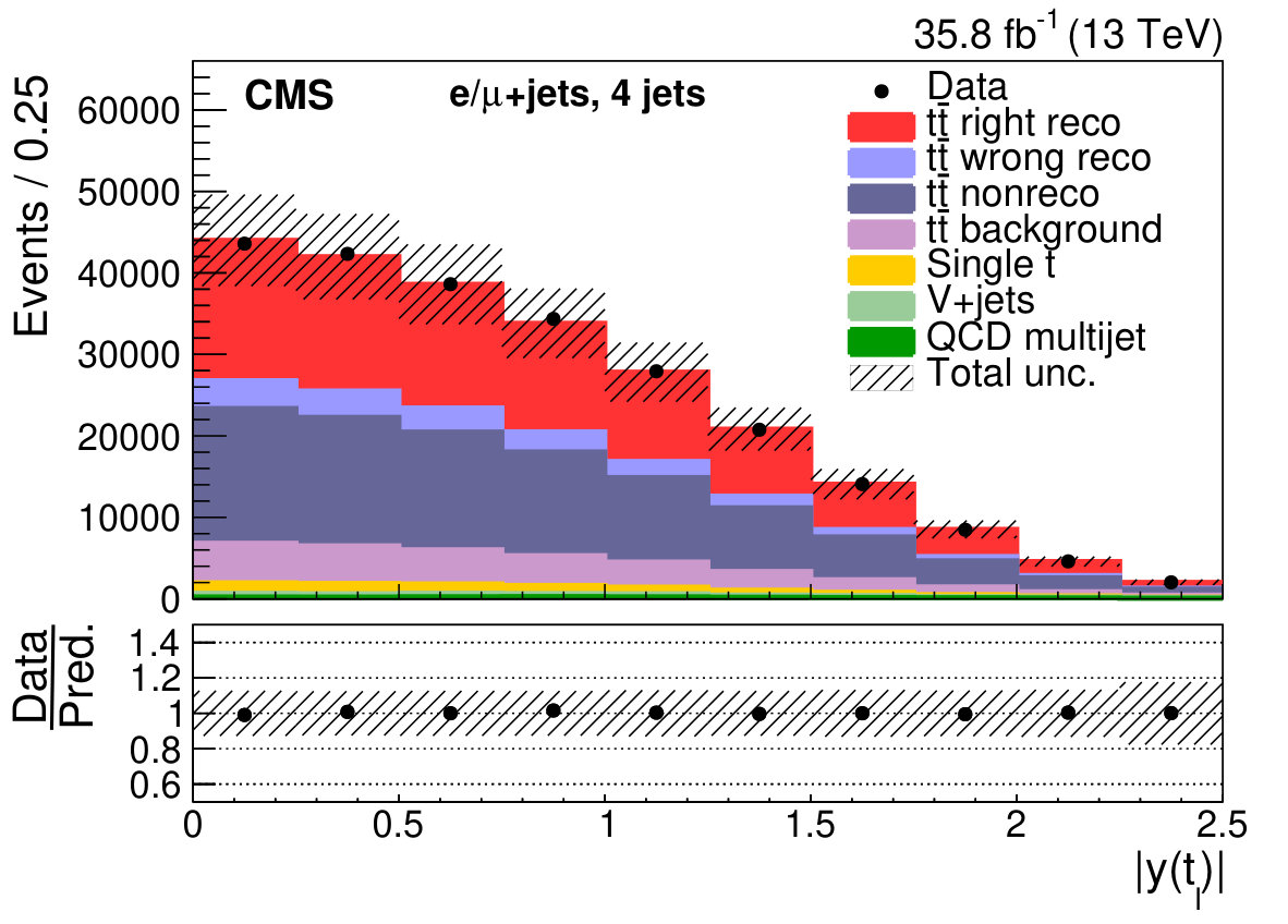 Figure 6
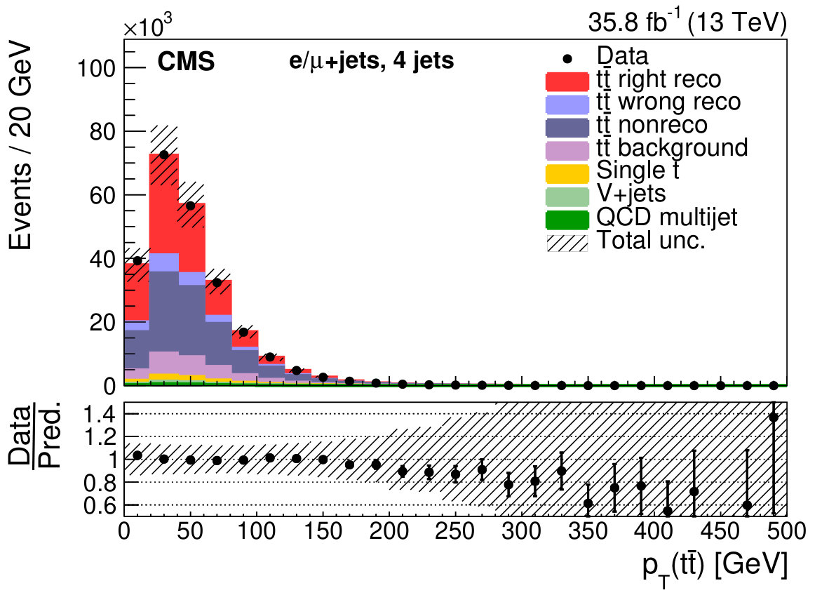 Figure 6
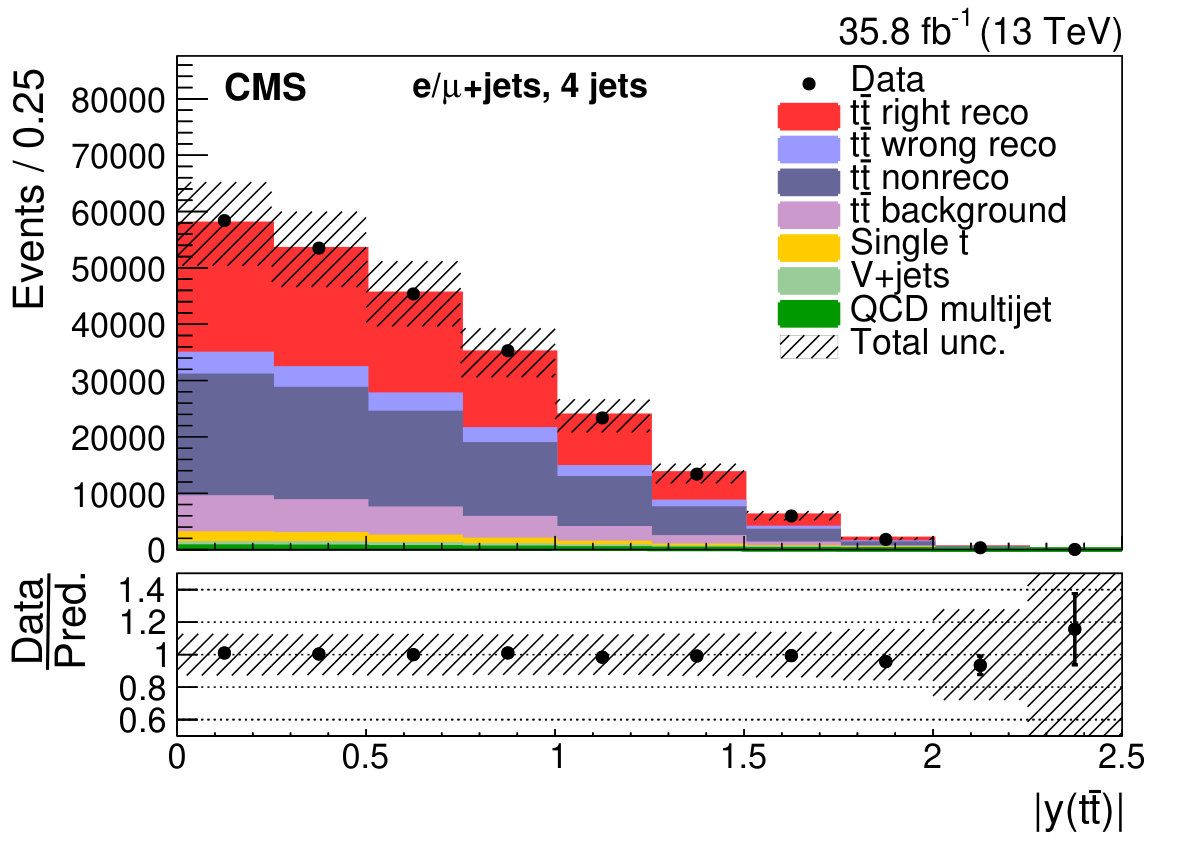 Figure 6
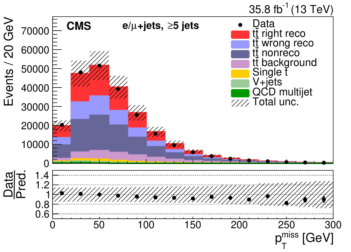 Figure 7
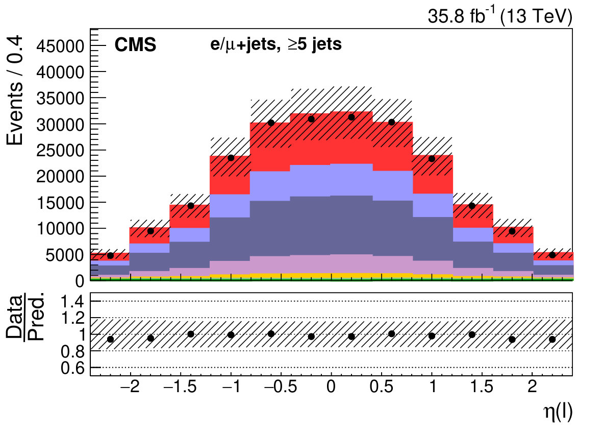 Figure 7
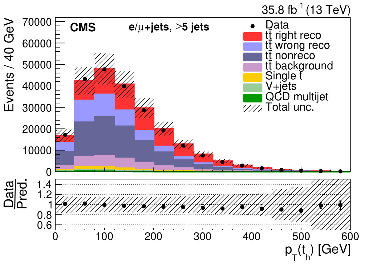 Figure 7
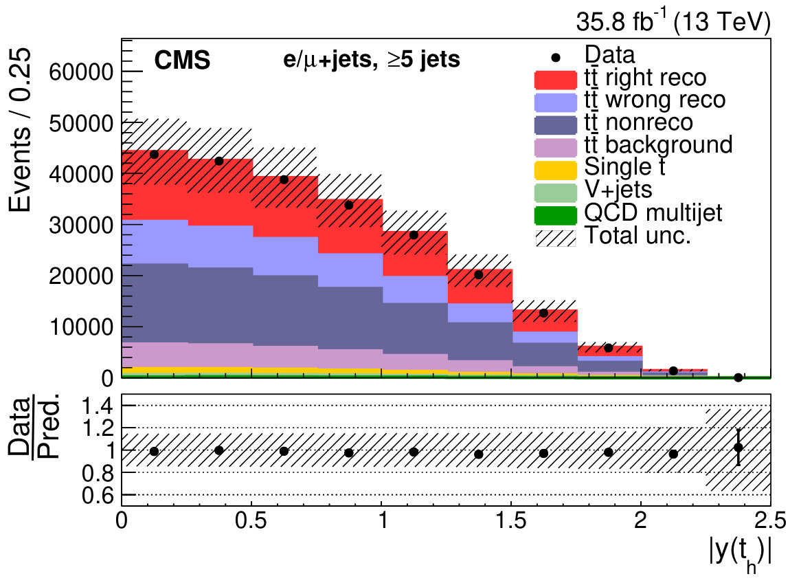 Figure 7
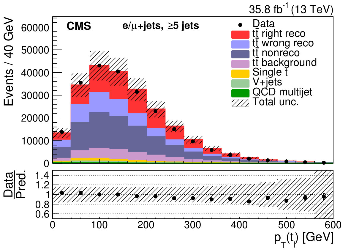 Figure 7
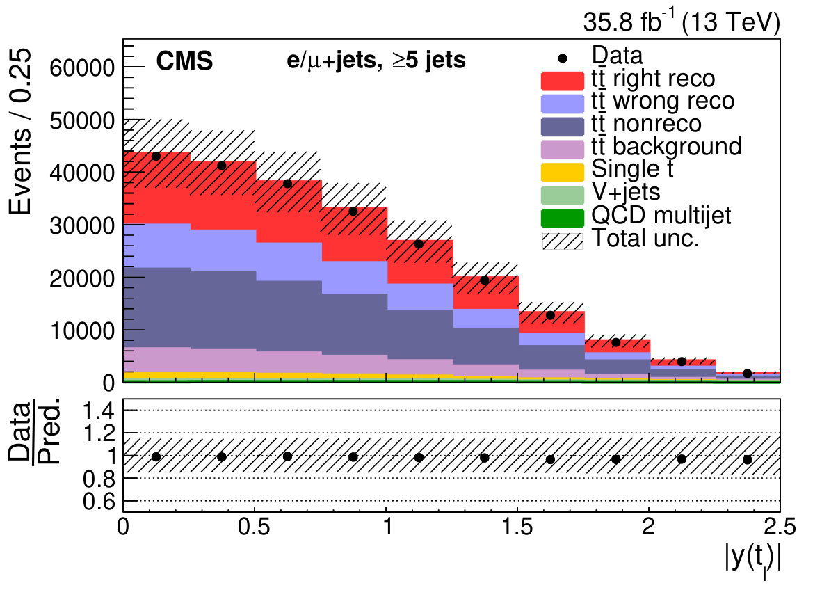 Figure 7
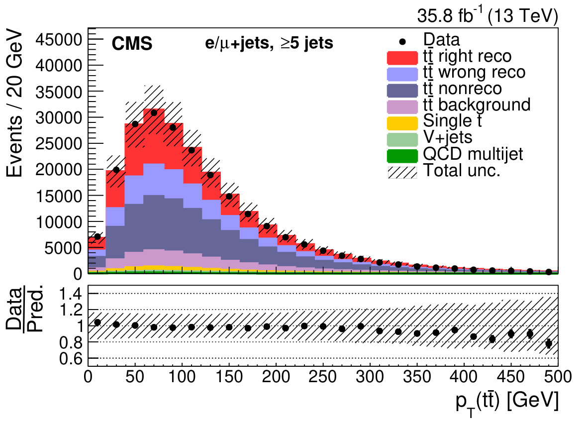 Figure 7
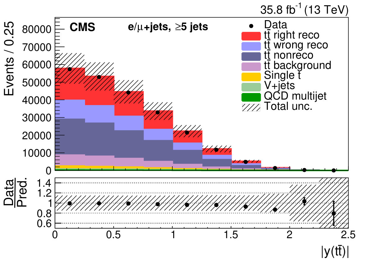 Figure 7
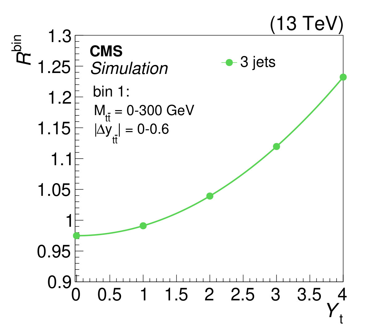 Figure 8
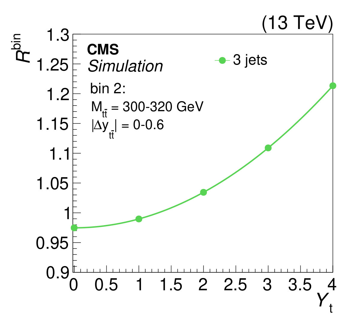 Figure 8
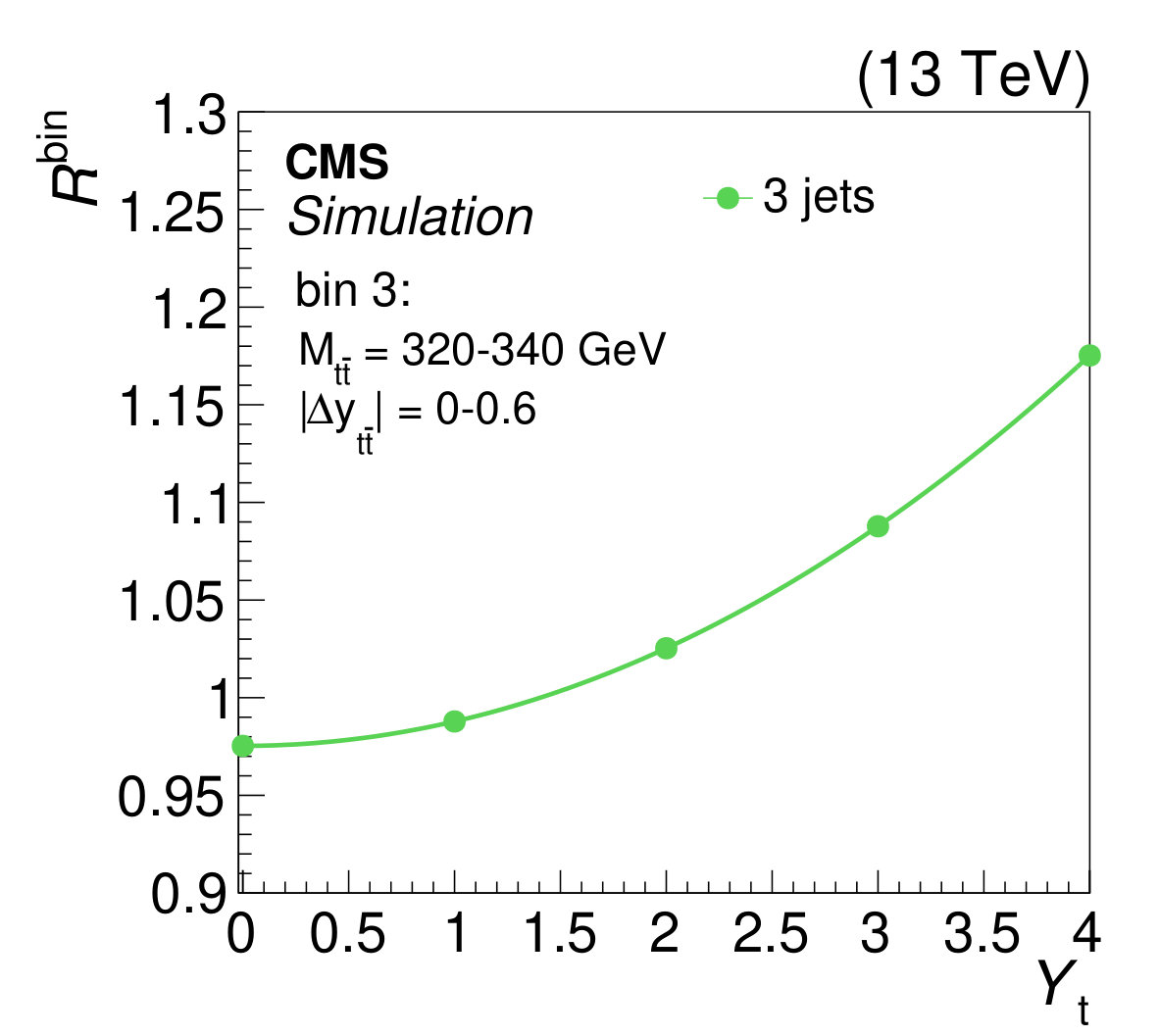 Figure 8
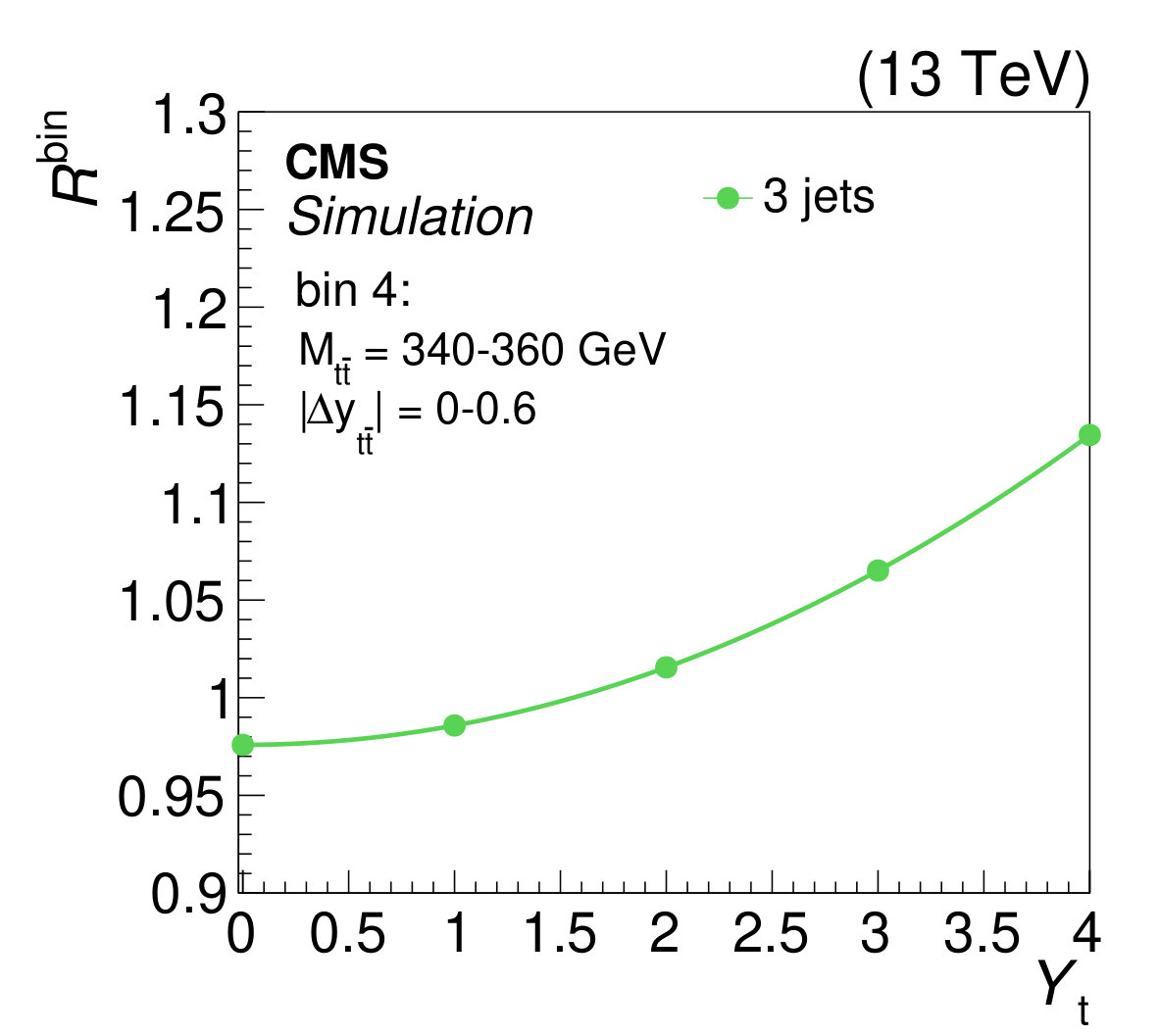 Figure 8
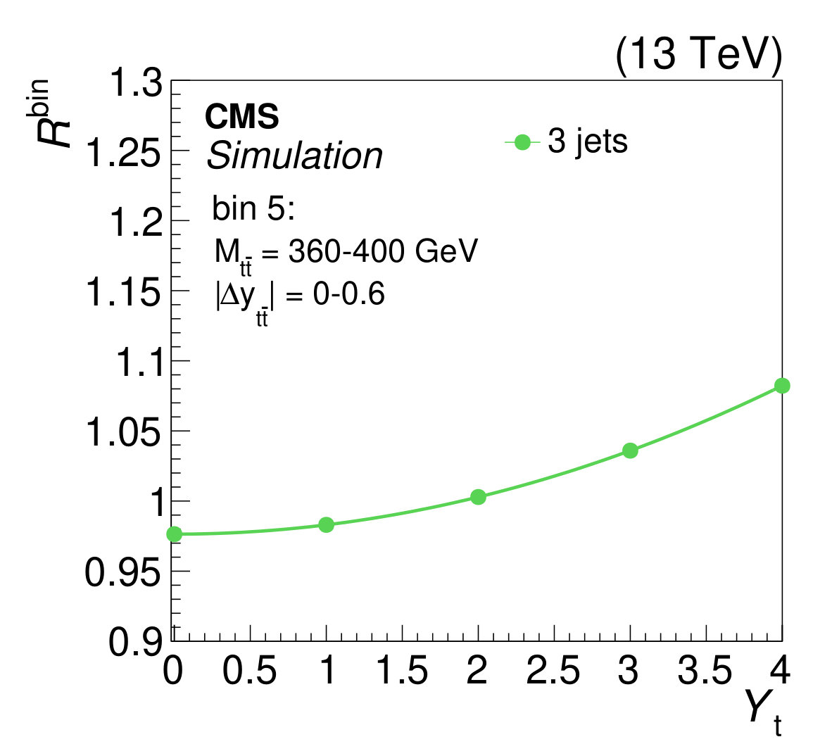 Figure 8
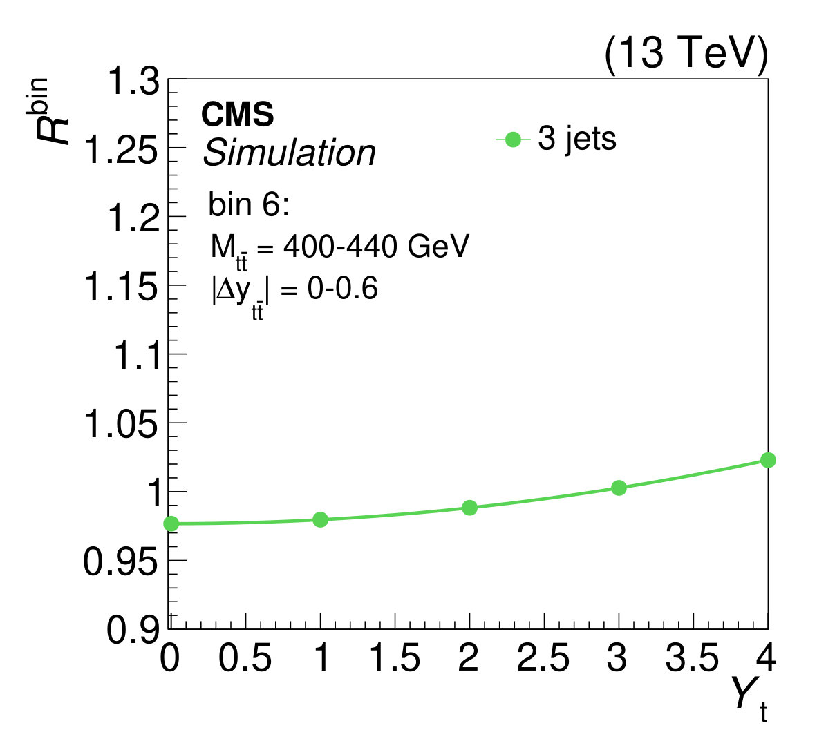 Figure 8
| (4) |
Peer Reviews
No public reviews on file for this paper yet. If you reviewed it on a platform where reviews are public (OpenReview, ICLR, NeurIPS, ICML), you can paste yours below so the community can read it here.
Videos
No videos yet. Explain this paper in a talk, walkthrough, or lecture? Add one.
\cmsNoteHeader
TOP-17-004
\RCS
\RCS \RCS
\cmsNoteHeader
TOP-17-004
Measurement of the top quark Yukawa coupling from \ttbar kinematic distributions in the lepton+jets final state in proton-proton collisions at
Abstract
Results are presented for an extraction of the top quark Yukawa coupling from top quark-antiquark (\ttbar) kinematic distributions in the lepton plus jets final state in proton-proton collisions, based on data collected by the CMS experiment at the LHC at , corresponding to an integrated luminosity of 35.8\fbinv. Corrections from weak boson exchange, including Higgs bosons, between the top quarks can produce large distortions of differential distributions near the energy threshold of \ttbarproduction. Therefore, precise measurements of these distributions are sensitive to the Yukawa coupling. Top quark events are reconstructed with at least three jets in the final state, and a novel technique is introduced to reconstruct the \ttbarsystem for events with one missing jet. This technique enhances the experimental sensitivity in the low invariant mass region, . The data yields in , the rapidity difference , and the number of reconstructed jets are compared with distributions representing different Yukawa couplings. These comparisons are used to measure the ratio of the top quark Yukawa coupling to its standard model predicted value to be with an upper limit of 1.67 at the 95% confidence level.
0.1 Introduction
The study of the properties of the Higgs boson, which is responsible for electroweak symmetry breaking, is one of the main goals of the LHC program. The standard model (SM) relates the mass of a fermion to its Yukawa coupling, \ie, the strength of its interaction with the Higgs boson, as , where is the fermion mass and is the vacuum expectation value of the Higgs potential [1], obtained from a measurement of the lifetime [2]. Since fermionic masses are not predicted by the SM, their values are only constrained by experimental observations. Given the measured value of the top quark mass of [3], the top quark is the heaviest fermion and therefore provides access to the largest Yukawa coupling, which is expected to be close to unity in the SM. It is important to verify this prediction experimentally. We define as the ratio of the top quark Yukawa coupling to its SM value. In this definition, is equal to as defined in the “ framework” [4], which introduces coupling modifiers to test for deviations in the SM couplings of the Higgs boson to other particles. Several Higgs boson production processes are sensitive to , in particular Higgs boson production via gluon fusion [5, 6] and Higgs boson production in association with top quark pairs, [7]. In both cases, in addition to , the rate depends on the Higgs boson coupling to the decay products, \eg, bottom quarks or leptons. The only Higgs boson production process that is sensitive exclusively to is production with the Higgs boson decaying to a \ttbarpair, leading to a four top quark final state [8]. In this paper, we explore a complementary approach to measure independently of the Higgs coupling to other particles by utilizing a precise measurement of the top quark pair production cross section, which is affected by a virtual Higgs boson exchange. It has been shown that in the top quark pair production threshold region, which corresponds to a small relative velocity between the top quark and antiquark, the \ttbarcross section is sensitive to the top quark Yukawa coupling through weak force mediated corrections [9]. For example, doubling the Yukawa coupling would lead to a change in the observed differential cross section comparable to the current experimental precision of around 6% [10]. A detailed study of the differential \ttbarkinematic properties close to the production threshold could, therefore, determine the value of the top quark Yukawa coupling. This approach is similar to the threshold scan methods proposed for \Pe+\Pe- colliders [11, 12].
We calculate the weak interaction correction factors for different values of using hathor (v2.1) [13] and apply them at the parton level to existing \ttbarsimulated samples. From these modified simulations, we obtain distributions at detector level that can be directly compared to data. The Yukawa coupling is extracted from the distributions of the invariant mass of the top quark pair, , and the rapidity difference between the top quark and antiquark, , for different jet multiplicities. The low and small regions are the most sensitive to .
Top quarks decay almost exclusively via and the final topology depends on the \PW boson decays. When one \PW boson decays leptonically and the other decays hadronically, + charge conjugate, the final state at leading order (LO) consists of an isolated lepton (electron or muon in this analysis), missing transverse momentum (from the neutrino), and four jets (from two \cPqb quarks and two light quarks). This final state has a sizable branching fraction of 34%, low backgrounds, and allows for the kinematic reconstruction of the original top quark candidates. This analysis follows the methodology employed in Ref. [14] and introduces a novel algorithm to reconstruct the \ttbarpair when only three jets are detected.
The outline of this paper is as follows. Section 0.2 introduces the method of implementing the weak force corrections in simulated events as well as the variables sensitive to the top quark Yukawa coupling. Section 0.3 describes the CMS detector. The data and simulated samples used in the analysis are described in Section 0.4. The event selection criteria are discussed in Section 0.5. The algorithm used to reconstruct \ttbarevents is described in Section 0.6. Details on background estimation and event yields are covered in Sections 0.7 and 0.8. The statistical methodologies and the systematic uncertainties are described in Sections 0.9 and 0.10, respectively. Section 0.11 presents the results of the fit to data. Section 0.12 summarizes the results.
0.2 Weak interaction corrections to \ttbar production
Recent calculations provide next-to-next-to-leading-order (NNLO) predictions within the framework of perturbative quantum chromodynamics (QCD) for the \ttbarproduction cross section [15, 16]. Photon-mediated corrections have been determined to be small [17]. The weak force corrections to the \ttbarproduction cross section were originally calculated [18] before the top quark discovery and were found to have a very small effect on the total cross section, so they are typically not implemented in Monte Carlo (MC) event generators. Nevertheless, they can have a sizable impact on differential distributions and on the top quark charge asymmetry. There is no interference term of order between the lowest-order strong force mediated and neutral current amplitudes in the quark-induced processes. The weak force corrections start entering the cross section at loop-induced order (as shown in Fig. 1). A majority of weak corrections do not depend on the top quark Yukawa coupling. Amplitudes linear in , which arise from the production of an intermediate -channel Higgs boson through a closed \cPqb quark loop, can be ignored because of the small \cPqb quark mass. However, the amplitude of the Higgs boson contribution to the loop ( in Fig. 1) is proportional to . The interference of this process with the Born-level \ttbarproduction has a cross section proportional to . Thus, in some kinematic regions, the weak corrections become large and may lead to significant distortions of differential distributions.
The hathor generator calculates the partonic cross section value, including the next-to-leading-order (NLO) weak corrections at order for given and . The mass of the top quark is fixed at , and its uncertainty is treated as a source of systematic uncertainty. We use hathor to extract a two-dimensional correction factor that contains the ratio of the \ttbarproduction cross section with weak corrections over the LO QCD production cross section in bins of and . This is done for different hypothesized values of , as shown in projections in Fig. 2. The largest effects arise near the \ttbarproduction threshold region and can be as high as 12% for = 2. We then apply this correction factor at the parton level as a weight to each \ttbarevent simulated with \POWHEG(v2) [19, 20, 21, 22]. In the distributions at the detector level, the experimental resolutions and the systematic uncertainties, which are especially significant in the low- region, will reduce the sensitivity to this effect.
0.3 The CMS detector
The central feature of the CMS detector is a superconducting solenoid of 6\unitm internal diameter, providing a magnetic field of 3.8\unitT. Within the solenoid volume are a silicon pixel and strip tracker, a lead tungstate crystal electromagnetic calorimeter (ECAL), and a brass and scintillator hadron calorimeter (HCAL), each composed of a barrel and two endcap sections. Forward calorimeters extend the coverage provided by the barrel and endcap detectors. Muons are measured in gas-ionization detectors embedded in the steel flux-return yoke outside the solenoid. A more detailed description of the CMS detector, together with a definition of the coordinate system and relevant kinematical variables, can be found in Ref. [23].
The particle-flow (PF) algorithm [24] reconstructs and identifies each individual particle with an optimized combination of information from the various elements of the detector systems. The energy of photons is directly obtained from the ECAL measurements, corrected for zero-suppression effects. The energy of electrons is determined from a combination of the electron momentum at the primary interaction vertex as determined by the tracker, the energy of the corresponding ECAL cluster, and the energy sum of all bremsstrahlung photons spatially compatible with originating from the electron track. The momentum of muons is obtained from the curvature of the corresponding track, combining information from the silicon tracker and the muon system. The energy of charged hadrons is determined from a combination of their momentum measured in the tracker and the matching ECAL and HCAL energy deposits, corrected for zero-suppression effects and for the response function of the calorimeters to hadronic showers. Finally, the energy of neutral hadrons is obtained from the corresponding corrected ECAL and HCAL energy. The reconstructed vertex with the largest value of the sum of the physics objects transverse momentum squared, , is taken to be the primary proton-proton (\Pp\Pp) interaction vertex.
0.4 Data set and modeling
The data used for this analysis corresponds to an integrated luminosity of 35.8\fbinvat a center-of-mass energy of 13\TeV. Events are selected if they pass single-lepton triggers [25]. These require a transverse momentum for electrons and for muons, each within pseudorapidity , as well as various quality and isolation criteria.
The MC event generator \POWHEGis used to simulate \ttbarevents. It calculates up to NLO QCD matrix elements and uses \PYTHIA(v8.205) [26] with the CUETP8M2T4 tune [27] for the parton shower simulations. The default parametrization of the parton distribution functions (PDFs) used in all simulations is NNPDF3.0 [28]. A top quark mass of 172.5\GeVis used. When compared to the data, the simulation is normalized to an inclusive \ttbarproduction cross section of \unitpb [29]. This value is calculated at NNLO accuracy, including the resummation of next-to-next-to-leading-logarithmic soft gluon terms. The quoted uncertainty is from the choice of hadronization, factorization, and renormalization scales and the PDF uncertainties.
The background processes are modeled using the same techniques. The \MGvATNLOgenerator [30] is used to simulate \PW boson and Drell–Yan (DY) production in association with jets and -channel single top quark production. The \POWHEGgenerator is used to simulate a single top quark produced in association with a \PW boson (), and \PYTHIAis used for QCD multijet production. In all cases, the parton shower and the hadronization are simulated by \PYTHIA. The \PW boson and DY backgrounds are normalized to their NNLO cross sections calculated with \FEWZ [31]. The cross sections of single top quark processes are normalized to NLO calculations [32, 33], and the QCD multijet simulation is normalized to the LO cross section from \PYTHIA. As explained in Section 0.7, the shape and the overall normalization of the QCD multijet contribution to the background are derived using data in a control region. The QCD multijet simulation is only used to determine relative contributions from different regions.
The detector response is simulated using \GEANTfour [34]. The same algorithms that are applied to the collider data are used to reconstruct the simulated data. Multiple proton-proton interactions per bunch crossing (pileup) are included in the simulation. To correct the simulation to be in agreement with the pileup conditions observed during the data taking, the average number of pileup events is calculated for the measured instantaneous luminosity. The simulated events are weighted, depending on their number of pileup interactions, to reproduce the measured pileup distribution.
0.5 Event reconstruction and selection
Jets are reconstructed from the PF candidates and are clustered by the anti-\ktalgorithm [35, 36] with a distance parameter . The jet momentum is determined as the vectorial sum of the momenta of all PF candidates in the jet. An offset correction is applied to jet energies to take into account the contribution from pileup within the same or nearby bunch crossings. Jet energy corrections are derived from simulation and are improved with in situ measurements of the energy balance in dijet, QCD multijet, photon+jet, and leptonically decaying \PZ+jet events [37, 38]. Additional selection criteria are applied to each event to remove spurious jet-like features originating from isolated noise patterns in certain HCAL and ECAL regions [39].
Jets are identified as originating from \cPqb quarks using the combined secondary vertex algorithm (CSV) v2 [40]. Data samples are used to measure the probability of correctly identifying jets as originating from \cPqb quarks (\cPqb tagging efficiency), and the probability of misidentifying jets originating from light-flavor partons (\cPqu, \cPqd, \cPqsquarks or gluons) or a charm quark as a \cPqb-tagged jet (the light-flavor and charm mistag probabilities) [40]. To identify a jet as a \cPqb jet, its CSV discriminant is required to be greater than 0.85. This working point yields a \cPqb tagging efficiency of 63% for jets with \pttypical of \ttbarevents, and charm and light-flavor mistag probabilities of approximately 12 and 2%, respectively (around 3% in total).
The missing transverse momentum, \ptvecmiss, is calculated as the negative vector sum of the transverse momenta of all PF candidates in an event. The energy scale corrections applied to jets are propagated to \ptvecmiss. Its magnitude is referred to as \ptmiss.
Candidate signal events are defined by the presence of a muon or an electron that is isolated from other activity in the event, specifically jets, and \ptvecmissassociated with a neutrino. The isolation variables exclude the contributions from the physics object itself and from pileup events. The efficiencies of lepton identification and selection criteria are derived using a tag-and-probe method in \ptand regions [41]. The same lepton isolation criteria described in Ref. [14] are followed here.
To reduce the background contributions and to optimize the \ttbarreconstruction, additional requirements on the events are imposed. Only events with exactly one isolated muon [42] or electron [43] with and are selected; no additional isolated muons or electrons with and are allowed; at least three jets with and are required, and at least two of them must be \cPqb tagged. The \PW boson transverse mass, defined as , is required to be less than 140\GeV, where is the transverse momentum of the lepton. For \ttbarevents with only three jets in the final state, the \ptof the leading \cPqb-tagged jet is required to be greater than 50\GeV.
0.6 Reconstruction of the top quark-antiquark system
The goal of reconstructing \ttbarevents is to determine the top quark and antiquark four-momenta. For this, it is necessary to correctly match the final-state objects to the top quark and antiquark decay products. We always assume that the two \cPqb-tagged jets with the highest CSV discriminant values are associated with the two \cPqbquarks from \ttbardecays. For each event, we test the possible assignments of jets as \ttbardecay products and select the one with the highest value of a likelihood discriminant constructed based on the available information.
The first step in building the likelihood discriminant is to reconstruct the neutrino four-momentum based on the measured \ptvecmiss, the lepton momentum , and the momentum of the jet associated with the \cPqbquark from the top quark decay. The neutrino solver algorithm [44] uses a geometric approach to find all possible solutions for the neutrino momentum based on the two mass constraints and . Each equation describes an ellipsoid in the three-dimensional neutrino momentum space. The intersection of these two ellipsoids is usually an ellipse. We select as the point on the ellipse for which the distance between the ellipse projection onto the transverse plane (,) and the measured \ptvecmissis minimal. The algorithm leads to a unique solution for the longitudinal component of the neutrino momentum and an improved resolution for its transverse component. When the invariant mass of the lepton and the candidate is above , no solution can be found and this jet assignment is discarded. If both candidates fail this requirement, then the event is rejected. The algorithm is applied for each of the two jet possibilities and the minimum distance is used to identify the correct jet in the leptonic top quark decay, , as described below.
0.6.1 Reconstruction of events with at least four jets
The likelihood discriminant for events with at least four reconstructed jets is built to minimize the calculated , and to simultaneously ensure that the invariant mass of the two jets hypothesized to originate from the \PW boson decay () is consistent with the \PW boson mass, and that the invariant mass of the three jets hypothesized to originate from the hadronically decaying top quark () is consistent with . The likelihood discriminant for events with at least four jets, , is constructed as
[TABLE]
where is the two-dimensional probability density to correctly reconstruct the \PW boson and top quark invariant masses, and is the probability density describing the distribution of for a correctly selected . On average, the distance for a correctly selected is smaller and has a lower tail compared to the distance obtained for other jets. Jet assignments with values of are rejected since they are very unlikely to originate from a correct association. The distributions from which and are derived, together with are shown in Figs. 2 (top-left), 2 (bottom-left) and 4 (left) of Ref. [14], respectively.
The efficiency of the reconstruction algorithm is defined as the probability that the most likely assignment, as identified by the largest value of , is the correct one, given that all decay products from the \ttbardecay are reconstructed and selected. Since the number of possible assignments increases drastically with the number of jets, it is more likely to select a wrong assignment if there are additional jets. The algorithm identifies the correct assignment in around 84% of the four-jet events, 69% of the five-jet events, and 53% of the six-jet events.
0.6.2 Reconstruction of events with exactly three jets
The most sensitive region of the phase space to probe the size of the top quark Yukawa coupling is at the threshold of \ttbarproduction. However, the efficiency for selecting \ttbarevents in this region is rather low, since one or more quarks from the \ttbardecay are likely to have \ptor outside of the selection thresholds resulting in a missing jet. To mitigate this effect, an algorithm was developed for the reconstruction of \ttbarevents with one missing jet [45].
As the missing jet in 93% of the selected three-jet events is associated with a quark from the \PW boson decay, we assume the two jets with the highest CSV discriminant are associated with \cPqb quarks from the \ttbardecay. The remaining two-fold ambiguity is in the assignment of the \cPqb-tagged jets: which one originates from the hadronic and which one from the semileptonic top quark decay. For each of the two possible \cPqb jet assignments, the algorithm uses the neutrino solver to calculate the corresponding minimum distance . If the neutrino solver yields no solution, this jet assignment is discarded and the other solution is used if available. Events with no solutions are discarded. If both \cPqb jet candidates have solutions for neutrino momentum, a likelihood discriminant is constructed using the minimum distance and the invariant mass of the two jets hypothesized to belong to the hadronic top quark decay. We choose the jet assignment with the lowest value of the negative log likelihood defined as
[TABLE]
where the label 3 refers to the requirement of three jets. The function is the probability density of to correctly identify , and is the probability density of the invariant mass of the hypothesized and the jet from the \PW boson decay. Figures 3 (left) and (middle) show the separation between correct and incorrect assignments in the relevant variables for signal events. The distribution of is shown in the right plot of Fig. 3. Jet assignments with values of are discarded to improve the signal-to-background ratio. Overall, this algorithm identifies the correct \cPqb jet assignment in 80% of three-jet events.
Semileptonic top quark decays are fully reconstructible, regardless of whether the event has three or four jets. The hadronically decaying top quark candidate in the missing jet category is approximated by the system of two jets identified to be associated with the hadronic top quark decay. Figure 4 shows the relative difference between the reconstructed and generated invariant mass of the \ttbarsystem and of the difference in rapidity for three-jet events, compared to those with four jets. Because of the missing jet, the observed value of in the three-jet category tends to be lower than in the four-jet category. However, this shift does not affect the measurement since the data are compared to the simulation in each different jet multiplicity bin: only the widths of these distributions are important. Figure 4 demonstrates that the three-jet reconstruction is competitive with the one achieved in the four-jet category.
To summarize, the newly developed three-jet reconstruction algorithm allows us to increase the yields in the sensitive low- region. As will be shown in Section 0.10, the addition of three-jet events also helps to reduce the systematic uncertainty from effects that cause migration between jet multiplicity bins, \eg, jet energy scale variation and the hadronization model. The analysis is performed in three independent channels based on the jet multiplicity of the event: three, four, and five or more jets.
0.7 Background estimation
The backgrounds in this analysis arise from QCD multijet production, single top quark production, and vector boson production in association with jets (V+jets). The expected number of events from and production is negligible and we ignore this contribution in the signal region (SR).
The contributions from single top quark and V+jets production are estimated from the simulated samples. Rather than relying on the relatively small simulated sample of QCD multijet events, smoother distributions in and are obtained from data in a control region (CR). Events in the CR are selected in the same way as the signal events, except that the maximum value of the CSV discriminant of jets in each event has to be less than 0.6. Hence, events in the CR originate predominately from V+jets and QCD multijet processes. The simulation in this background-enriched CR describes the data well within uncertainties. We take the distributions in and from data in the CR, after subtracting the expected contribution from the V+jets, single top quark, \ttbar, and and processes. To obtain distributions in the SR, the distributions in the CR are then normalized by the ratio of the number of events in the SR () and CR () determined from simulated QCD multijet events:
[TABLE]
where is the residual yield in data (after subtracting the background contributions not from QCD multijet). The SR-to-CR simulated events ratio in Eq. (3) is 0.043 0.014, 0.041 0.012, and 0.081 0.015 for three, four, and five or more jets, respectively. The normalization uncertainty is estimated to be 30%. The shape uncertainty due to the CR definition is evaluated by selecting events for which the lepton fails the isolation requirement. The uncertainty is defined by the difference between the distributions of events that pass or fail the CSV discriminant requirement and can be as large as 60% in some regions of phase space.
0.8 Event yields and control plots
Table 0.8 shows the expected and observed event yields after event selection and \ttbarreconstruction, including the statistical uncertainties in the expected yields. All of the \ttbarcomponents depend on the top quark Yukawa coupling from the production, so all of them are considered as signal. Here, the signal simulation is divided into the following categories: correctly reconstructed \ttbarsystems (\ttbarright reco); events where all required decay products are available, but the algorithm failed to identify the correct jet assignments (\ttbarwrong reco); +jets \ttbarevents where at least one required decay product is missing (\ttbarnonreconstructible); and \ttbarevents from dileptonic, , or fully hadronic decays (\ttbarbackground).
The reference list from the paper itself. Each links out to its DOI / PubMed record.
- 1[1] S. Weinberg, “A model of leptons”, Phys. Rev. Lett. 19 (1967) 1264, 10.1103/Phys Rev Lett.19.1264 . · doi ↗
- 2[2] Mu Lan Collaboration, “Measurement of the positive muon lifetime and determination of the Fermi constant to part-per-million precision”, Phys. Rev. Lett. 106 (2011) 041803, 10.1103/Phys Rev Lett.106.041803 , ar Xiv:1010.0991 . [Erratum: \DOI 10.1103/Phys Rev Lett.106.079901]. · doi ↗
- 3[3] CMS Collaboration, “Measurement of the top quark mass using proton-proton data at s 𝑠 \sqrt{s} = 7 and 8 Te V”, Phys. Rev. D 93 (2016) 072004, 10.1103/Phys Rev D.93.072004 , ar Xiv:1509.04044 . · doi ↗
- 4[4] LHC Higgs Cross Section Working Group Collaboration, “Handbook of LHC Higgs cross sections: 3. Higgs properties”, (2013). ar Xiv:1307.1347 .
- 5[5] CMS Collaboration, “Measurements of properties of the Higgs boson decaying into the four-lepton final state in pp collisions at s 𝑠 \sqrt{s} = 13 Te V”, JHEP 11 (2017) 047, 10.1007/JHEP 11(2017)047 , ar Xiv:1706.09936 . · doi ↗
- 6[6] CMS Collaboration, “Measurements of Higgs boson properties in the diphoton decay channel in proton-proton collisions at s 𝑠 \sqrt{s} = 13 Te V”, JHEP 11 (2018) 185, 10.1007/JHEP 11(2018)185 , ar Xiv:1804.02716 . · doi ↗
- 7[7] CMS Collaboration, “Observation of t t ¯ t ¯ t \mathrm{t\overline{t}} H production”, Phys. Rev. Lett. 120 (2018) 231801, 10.1103/Phys Rev Lett.120.231801 , ar Xiv:1804.02610 . · doi ↗
- 8[8] CMS Collaboration, “Search for standard model production of four top quarks with same-sign and multilepton final states in proton-proton collisions at s = 13 Te V 𝑠 13 Te V \sqrt{s}=13\,\text{Te V} ”, Eur. Phys. J. C 78 (2018) 140, 10.1140/epjc/s 10052-018-5607-5 , ar Xiv:1710.10614 . · doi ↗