Geometric and Obstacle Scattering at Low Energy
Alexander Strohmaier, Alden Waters

TL;DR
This paper analyzes low-energy scattering of differential forms on Riemannian manifolds with obstacles, revealing eigenforms and resonances at zero energy, with explicit expansions and applications to electromagnetic wave scattering.
Contribution
It provides explicit low-energy expansions of the resolvent, scattering matrix, and spectral measure for differential forms on manifolds with obstacles, including new resonance phenomena and a Birman-Krein formula.
Findings
Eigenforms appear in the expansion near zero energy.
In dimension two, an additional resonance occurs due to obstacles.
The expansions involve λ and log λ, described using Hahn holomorphic functions.
Abstract
We consider scattering theory of the Laplace Beltrami operator on differential forms on a Riemannian manifold that is Euclidean at infinity. The manifold may have several boundary components caused by obstacles at which relative boundary conditions are imposed. Scattering takes place because of the presence of these obstacles and possible non-trivial topology and geometry. Unlike in the case of functions eigenvalues generally exist at the bottom of the continuous spectrum and the corresponding eigenforms represent cohomology classes. We show that these eigenforms appear in the expansion of the resolvent, the scattering matrix, and the spectral measure in terms of the spectral parameter near zero, and we determine the first terms in this expansion explicitly. In dimension two an additional cohomology class appears as a resonant state in the presence of an obstacle. In even…
Click any figure to enlarge with its caption.
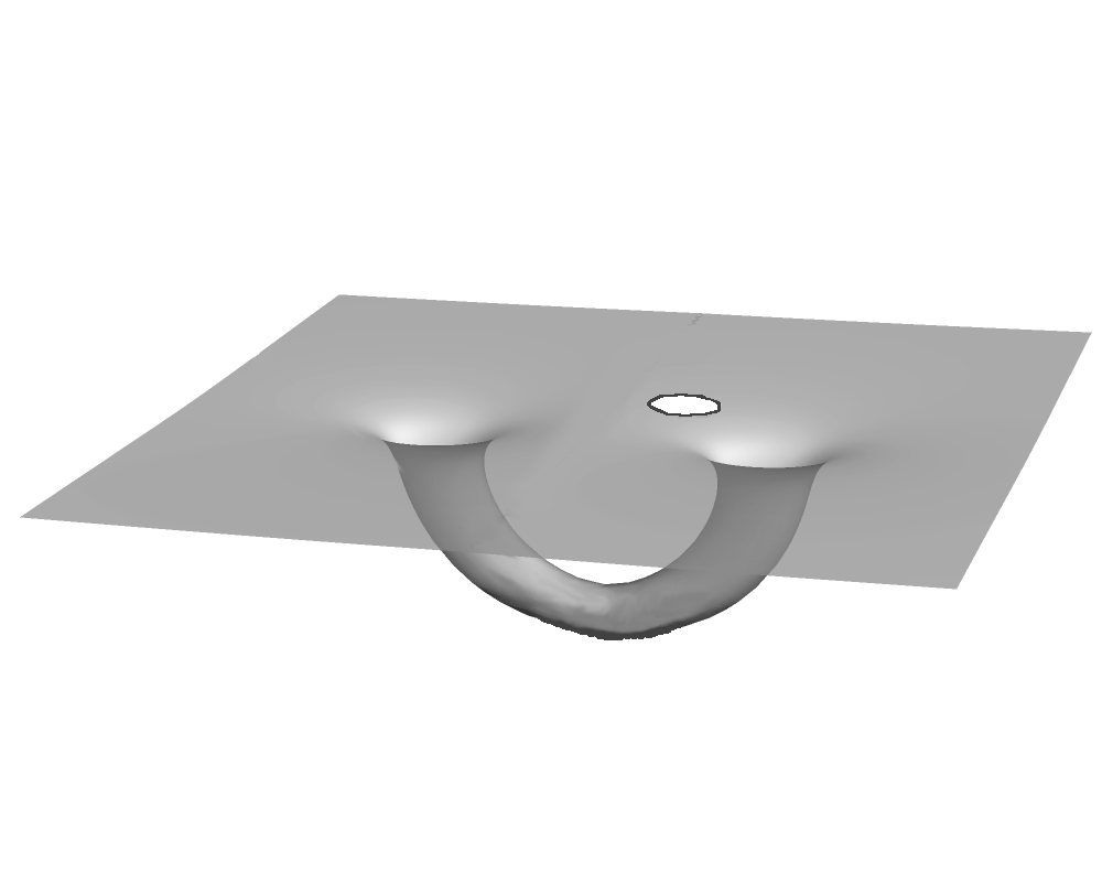 Figure 1
Peer Reviews
No public reviews on file for this paper yet. If you reviewed it on a platform where reviews are public (OpenReview, ICLR, NeurIPS, ICML), you can paste yours below so the community can read it here.
Videos
No videos yet. Explain this paper in a talk, walkthrough, or lecture? Add one.
Geometric and Obstacle Scattering at Low Energy
Alexander Strohmaier
School of Mathematics, University of Leeds, Leeds , Yorkshire, LS2 9JT, UK
and
Alden Waters
University of Groningen, Bernoulli Institute, Nijenborgh 9, 9747 AG Groningen, The Netherlands
Abstract.
We consider scattering theory of the Laplace Beltrami operator on differential forms on a Riemannian manifold that is Euclidean at infinity. The manifold may have several boundary components caused by obstacles at which relative boundary conditions are imposed. Scattering takes place because of the presence of these obstacles and possible non-trivial topology and geometry. Unlike in the case of functions eigenvalues generally exist at the bottom of the continuous spectrum and the corresponding eigenforms represent cohomology classes. We show that these eigenforms appear in the expansion of the resolvent, the scattering matrix, and the spectral measure in terms of the spectral parameter near zero, and we determine the first terms in this expansion explicitly. In dimension two an additional cohomology class appears as a resonant state in the presence of an obstacle. In even dimensions the expansion is in terms of and . The theory of Hahn holomorphic functions is used to describe these expansions effectively. We also give a Birman-Krein formula in this context. The case of one forms with relative boundary conditions has direct applications in physics as it describes the scattering of electromagnetic waves.
Supported by Leverhulme grant RPG-2017-329
Contents
-
3.1.1 Resolvent expansion and generalised eigenforms in dimension three
-
3.1.2 Resolvent expansion and generalised eigenforms in dimension five
-
6 The Birman-Krein formula and expansions of the spectral shift function
1. Introduction and Setting
The analysis of the spectrum and the spectral decomposition of geometric operators on manifolds is important in both physics and mathematics. A full spectral decomposition allows one to solve linear equations such as the wave equation, Schrödinger’s equation, and the heat equation. The long term behaviour of the latter is determined by the bottom of the spectrum. For the Laplace operator on -forms on a closed Riemannian manifold the Hodge isomorphism ([23]) identifies the harmonic forms with the de-Rham cohomology groups. Such connections between the bottom of the spectrum of geometric operators on closed manifolds give rise to an extremely rich interplay between topology and the analysis of partial differential equations. One of the important examples is the Atiyah-Singer index theorem ([1]) that relates the index of an elliptic operator to the -theory class determined by its principal symbol. On non-compact manifolds the situation is slightly more complicated due to the presence of an essential spectrum. One approach to analyse the topology of the space using Hodge theory is to study -cohomology which in many examples can be identified with the space of -harmonic forms, i.e. the zero eigenspace of the Laplace operator. Well-studied examples are manifolds with cylindrical ends ([2, 27]), cusp-ends and variants of these ([27, 40, 21]), as well as manifolds with conical singularities ([8]) and conical ends ([29]). To illustrate this we briefly explain the situation for manifolds with cylindrical ends. Here there may be a finite dimensional space of -eigenfunctions at zero, but in general zero is also contained in the absolutely continuous spectrum. The -harmonic forms on the manifold describe the image of cohomology with compact support in the cohomology of the space. A complement of this image can be described by the values of the generalised eigenfunctions at zero. This relation between cohomology and the low lying values of the continuous part of the spectral decomposition was somewhat anticipated by the work of Atiyah Patodi and Singer ([2]) on the index theorem for manifolds with boundary. The relationship between these concepts was further clarified by Melrose ([27]) and Müller ([32]). A detailed analysis of the bottom of the continuous spectrum for manifolds with cylindrical ends can be found in ([33]).
Another class of important examples are manifolds with conical ends and the subclass of manifolds with one Euclidean end. Similarly to the case of cylindrical ends the -cohomology groups can be identified with the zero eigenspace of the Laplace operator on forms. These groups can be computed here within a very general framework and related to de-Rham cohomology groups c.f. also ([29, 6, 21]).
The goal of this paper is to clarify the role of the continuous spectrum in this context. Namely, we analyse the spectral decomposition of the Laplace-Beltrami operator acting on -forms on oriented manifolds that are asymptotically Euclidean at infinity and with possible compact boundary on which relative boundary conditions are imposed. The boundary components are thought of as obstacles and scattering takes place because of these obstacles, and possibly because of a non-trivial geometry and topology.
The spectrum of lies on the positive real line. It consists of an absolutely continuous part, described by generalised eigenfunctions, and possibly a zero eigenvalue of finite multiplicity given by the -Betti numbers. In fact the space of -harmonic forms has a finer filtration that we describe in this paper that encodes how fast the corresponding eigenfunctions decay at infinity. In dimensions the structure of the singularities of the resolvent, the spectral measure and the scattering matrix, can be completely characterised in terms of the -eigenfunctions and their decay properties. Some information about the cohomology of the manifold is therefore retained in the continuous spectrum. In the case when the boundary is non-empty there is a non-trivial cohomology class in relative cohomology that is not represented by an -harmonic form but rather by a zero resonant state. We completely clarify the singularity structure of the resolvent near zero and its meromorphic continuation. We also give the leading term in the expansion of the scattering amplitude. In even dimensions, the resolvent, the scattering matrix, and the generalised eigenfunctions, are not holomorphic at zero but have convergent generalised expansions into power series containing both powers of and . The theory of these functions was developed in [31] and this paper makes extensive use of this theory. Our approach is similar to that of Vainberg [41] in its treatment of logarithmic terms.
The low energy behaviour of Schrödinger operators has been studied by Kato and Jensen ([24]) who also computed expansion coefficients for the resolvent in various dimensions (see for example [25]). Murata ([34]), using also the method of Vainberg ([41]) analysed the low energy behaviour of constant coefficient operators with potentials. The two dimensional case is quite complicated and was analysed for potential scattering in great detail in [3].
Resolvent expansions in the more general setting of conical ends were given by Wang ([46, 45]). Perhaps closest to our results are expansions obtained in the works by Guillarmou and Hassell ([17, 18]) where various resolvent expansions for the Laplace operator on functions are proved in the setting of conical manifolds. In [18] the authors compute one of the expansion coefficients in the resolvent in the case of functions and reproduce the formula of Jensen and Kato in this more general setting. Expansions for differential forms were used in [19]) to show boundedness of the Riesz transform on -spaces. Other recent work discussing the low energy behaviour of the resolvent is by Bony and Häfner [4] for second order operators in divergence form, and by Rodnianski and Tao [38] who also consider potentials and general asymptotically conic manifolds. We would also like to mention the very recent work of Vasy on the low energy resolvent on asymptotically conic spaces ([42], [43], [44]) and the fact that the long time behaviour of solutions of the wave equation on differential forms also plays a role in stability questions in general relativity ([22, 20]).
A relation between the topology of manifolds with Euclidean ends and the continuous spectrum has been noticed by Carron who gives expansions of the determinant of the scattering matrix in terms of -Betti numbers and resonant states ([7]), which shows in particular that the jump of the spectral shift function at zero is of topological significance. The significance of the spectral shift function in this context was also seen by Borisov Mueller and Schrader in their proof of the Chern-Gauss-Bonnet formula for asymptotically Euclidean manifolds ([5]). The detailed structure of the resolvent on non-compact manifold is also important in quantum field theory in the quantisation of the electromagnetic field as poles of the resolvent manifest themselves as “infrared problems”. As an example the Gupta-Bleuler quantisation of the electromagnetic field as constructed rigorously in [14, 15] requires the absence of a zero resonance state for the Laplace operator on one forms.
1.1. Precise setup and notations
Let be an oriented complete connected Riemannian manifold of dimension which is Euclidean at infinity, i.e. there exists compact subsets and such that is isometric to . Let be an open subset in with compact closure and smooth boundary. The (finitely many) connected components will be denoted by with some index . We will think of these as obstacles placed in . Removing these obstacles from results in a Riemannian manifold with smooth boundary . We will assume throughout that is connected, that the so that the obstacles are contained in . We will also fix the isometry to so that we have a natural coordinate system on .
Let as usual be the differential on smooth forms and its formal adjoint. The Laplace-Beltrami operator on differential forms is defined as . We denote the restriction to forms of degree by . There are natural boundary conditions that can be imposed on to make this into an essentially self-adjoint operator which we now describe. For a differential form we denote its restriction to by . If is the natural inclusion map the restriction is therefore a section in the pull back bundle . This bundle is canonically isomorphic to , the induced splitting being the split of into tangential and normal components . The tangential component is the same as the pull-back of the differential form to . There are several distinguished boundary conditions for the Laplace operator that lead to self-adjoint extensions of the Laplace operator on compactly supported smooth forms. Relative boundary conditions for the Laplace operator are defined as
[TABLE]
Absolute boundary conditions are defined to be
[TABLE]
Note that if satisfies relative boundary conditions, then satisfies absolute boundary conditions. Here is the Hodge star operator.
We will denote by and the self-adjoint extensions of unbounded operators in of resulting from the respective boundary conditions. Since the Hodge star operator allows us to pass from relative to absolute boundary conditions. The relative Laplacian acting on differential forms can be written as the square of a self-adjoint operator (see for example [12, 16, 5]). Here is the closure of the operator , and is the closure of the restriction of . Here is the interior of .
If the relative boundary conditions correspond to Dirichlet boundary conditions imposed on , and absolute boundary conditions correspond to Neumann boundary conditions.
The Hilbert space decomposes orthogonally into three invariant subspaces for as follows (see [12] and also [16])
[TABLE]
where is the space of relative -harmonic -forms, i.e. the space of square integrable forms that are closed, co-closed and satisfy relative boundary conditions.
The case is of particular interest in scattering theory of the electromagnetic field. Here the physics of the electromagnetic field in radiation gauge in the absence of charges and currents with the obstacles being perfect conductors is described by the operator on co-closed forms. To be more precise, the electromagnetic vector potential of a scattering wave in the frequency domain will satisfy relative boundary conditions and will be co-closed. It will also be a generalized eigenfunction of as expressed by the Helmholtz equation . The detailed spectral resolution and the scattering theory of therefore describes scattering of electromagnetic waves in geometric backgrounds with perfectly conducting obstacles.
The spaces are finite dimensional and directly related to the singular relative cohomology groups with compact support and coefficients in as follows. If then we have natural isomorphisms
[TABLE]
Similarly, for the absolute boundary conditions one obtains for
[TABLE]
These statements follow from a more general theorem by Melrose for scattering manifolds (as a consequence of Theorem 4 in case in [29]) and Carron who analysed the asymptotically flat case in great detail. In particular, the statement above can be inferred using the exact sequence of Theorem 4.4 combined with Lemma 5.4 in [6]. In dimension we have
[TABLE]
which follows from Proposition 5.5 in [6]. Moreover, the dual statement is
[TABLE]
The dimensions of these spaces, the -Betti numbers, are therefore computable using the Mayer-Vietoris sequence. Note that it follows from the long exact sequence in cohomology that for manifolds Euclidean at infinity we always have if . For a more detailed description of the above natural isomorphisms see for example [6].
Example 1.1**.**
If and consists of non-intersecting balls, one obtains for that . These are the only non-trivial spaces of harmonic forms satisfying relative boundary conditions. In the case , one has .
Example 1.2**.**
A wormhole in is obtained by removing two non-intersecting balls and gluing the resulting spheres. In this case one obtains and as the only non-trivial spaces of square integrable harmonic forms.
Example 1.3**.**
Another interesting example is when is a full torus. In this case we also have and as the only non-trivial spaces of relative harmonic forms.
In terms of -Betti numbers the examples 1.2 and 1.3 cannot be distinguished. We will see later that a certain refinement taking into account the decay properties of the harmonic forms distinguishes these spaces.
Choose an orthonormal basis in consisting of eigensections. If is the orthogonal projection onto we have
[TABLE]
Each eigenfunction admits a multipole expansion
[TABLE]
if is an orthonormal basis consisting of spherical harmonics of degree , c.f. Appendix D. For define
[TABLE]
whenever the sum converges absolutely. In particular the sum is finite when is a finite linear combination of spherical harmonics. For each we can also define the matrices
[TABLE]
The do not depend on the choice of orthonormal basis but they depend on the choice of orthonormal basis in . However, the maps
[TABLE]
are invariantly defined and self-adjoint.
Suppose is a harmonic form with a multipole expansion on of the form
[TABLE]
in case or
[TABLE]
in case . We then define
[TABLE]
Note that .
Whereas gives the discrete part of the spectrum, the continuous part of the spectrum is described by the generalised eigenfunction that are indexed by . For fixed these generalised eigenfunctions are completely determined by their asymptotic behaviour
[TABLE]
where and is the pull-back of the antipodal map. The map is called the scattering matrix, and is called the scattering amplitude.
1.2. Statement of the main theorems
Suppose that are functions that take values in a locally convex topological vector space and . As usual we write if for every continuous semi-norm on there is a constant such that for all .
Theorem 1.4**.**
Let be defined by
[TABLE]
and suppose that is a spherical harmonic of degree , then the generalised eigenfunctions have for small and bounded the following expansions
- •
For ,
[TABLE]
- •
For ,
[TABLE]
- •
For ,
[TABLE]
In any dimension, if or , then and therefore in the previous expansions.
This shows that all -eigenfunctions appear as expansion coefficients of generalised eigenfunctions. Note that in even dimensions the functions are defined on a logarithmic cover of the complex plane and the estimates are understood as functions in an arbitrary but fixed sector of this cover (see Section A). Hence the need for the restriction to bounded .
Theorem 1.5**.**
If is odd and the resolvent (as an operator from to ) has for small an expansion of the form
[TABLE]
where is holomorphic near zero. If then , and in particular we have that if . If is odd and then .
The situation in even dimensions is different. In this case the resolvent (as an operator from to ) is Hahn meromorphic at zero, i.e. it has a convergent expansion in terms of powers of and (see Appendix A for the precise definition of this notion).
Theorem 1.6**.**
If is even and then the resolvent, as an operator from to , takes for small and bounded the form
[TABLE]
where is Hahn-holomorphic and if , and if .
We now summarise the results for the two dimensional case.
Theorem 1.7**.**
Suppose that and either or . Then the resolvent, as an operator from to , takes for small and bounded the form
[TABLE]
where is Hahn-holomorphic. If and then , where is a constant function one. If then . In case we have , where is the volume form.
The results in the case of one-forms in dimension two are rather complicated and require the definition of certain natural functions. First note that if is a linear function on then is a harmonic one form of degree zero. It turns out that there is a harmonic function that satisfies relative boundary conditions such that
[TABLE]
By the maximum principle is uniquely determined up to a constant and therefore is well-defined. Note that is a one-form that satisfies relative boundary conditions and, since the multipole expansion (see Appendix D) can be differentiated, we have
[TABLE]
Let be the constant function . In case there is a boundary, i.e. , there exists a unique harmonic function satisfying Dirichlet boundary conditions such that
[TABLE]
for sufficiently large. We then have is closed and co-closed, satisfies relative boundary conditions, and
[TABLE]
where we have again used that the multipole expansion may be differentiated.
Theorem 1.8**.**
Suppose that and . Let be a spherical harmonic of degree . Let in case and define otherwise. Then, for small and bounded we have
- •
if we have
- •
if we have
[TABLE]
Note that if .
Theorem 1.9**.**
If and the resolvent, as an operator from to , has an expansion for small and bounded of the form
[TABLE]
where is Hahn holomorphic and is the Euler-Mascheroni constant. Here in case , and if . Moreover, we have
[TABLE]
The form is, by construction, a cohomology class that generates the image of the map . This image is not detected by -cohomology theory in the two dimensional case and the above shows that this cohomology class appears as a zero-energy resonant state instead.
Each of the expansions of the generalised eigenfunctions can be used to derive an expansion of the scattering matrix and the scattering amplitude. Section 4 describes the detailed expansion depending on the dimension. The leading order behavior is independent of the dimension and can be summarised into the following theorem.
Theorem 1.10**.**
If and is a spherical harmonic of degree , then
[TABLE]
where for small and bounded we have
- •
* if ,*
- •
* if ,*
- •
* if .*
If , then , in particular for any and small and bounded .
The two dimensional case is more involved due to the existence of a zero resonant state when . In this case we have for any . Precise expansions depend on the form degree and the presence of an obstacle.
Theorem 1.11**.**
If and is a spherical harmonic of degree , then, for small and bounded , we have
- •
if or then and
[TABLE]
- •
if , using the notation of Theorem 1.8,
[TABLE]
The expansions of the generalised eigenfunctions encode the finer structure on the space given by the order of vanishing at infinity. Indeed, the space carries a natural filtration
[TABLE]
where , defined for , is the space of -harmonic forms satisfying relative boundary conditions whose multipole expansion only has nonzero terms of order . In parts this filtration has topological significance.
Theorem 1.12**.**
If and then isomorphic to the kernel of the map . In particular if or , and if and .
By the long exact sequence in cohomology the kernel of is the same as the image of the map . This map is given by the limit of a the generalised eigenfunction (see Section 5). The fact that these spaces are isomorphic can probably also be inferred from the general framework [27]. As explained before this is not true in dimension two where this image shows up as a zero resonance state.
Finally, we give a short proof of the relative Birman-Krein formula in our setting with particular emphasis on the low energy behaviour. The expansions of the scattering amplitudes therefore directly translate into the asymptotic properties of the spectral shift function (see Section 6 for a definition) which is expressed as
[TABLE]
where
[TABLE]
the integer is the -Betti number, and equals one in case and zero otherwise. The jump of the spectral shift function at zero was also computed by Carron in [7] using a different method. The expansions of can be used to prove refined expansions for the spectral shift function at zero. An example is the following theorem.
Theorem 1.13**.**
Suppose . Then we have for the estimate
[TABLE]
where in case we have , in case we have , and finally .
Similar expansions can be derived in dimension two. The details of the expansions of the spectral shift function and their applications will be discussed elsewhere.
1.3. Plan of the paper
The paper is organised as follows. Section 2 gives a review of basic spectral theory for the Hodge Laplacian on -forms with boundary conditions. It develops the theory of generalised eigenfunctions based on Bessel function expansions, and it states the main spectral decomposition results that relate the generalised eigenfunctions, the resolvent, and the scattering matrix. Section 3 establishes the main technical lemmata to derive low energy expansions of the resolvent and the generalised eigenfunctions. Section 4 employs the obtained expansions for the resolvent and the eigenfunction expansions to derive expansions for the scattering amplitude. In Section 5 we establish the relation between cohomology and the low energy expansions of the generalised eigenfunctions. Finally, we give a proof of the Birman-Krein formula in our setting in Section 6. Since the main theorems require lengthy arguments in parts bootstrapping we have decided to summarise them in the introduction and explain in Section 7 in detail how they are obtained from the main body of the text.
1.4. Possible generalisations
For the purposes of this article we have focused on the important case of compact perturbations of Euclidean space. This is also the case that is most relevant in physics. There are two natural generalisations of this. One is to consider compact perturbations of globally symmetric spaces. In this case the theory of Hahn meromorphic functions can still be applied with a difference being that the bottom of the continuous spectrum is generally not at zero any more and therefore the cohomological interpretation will be lost. Another generalisation is to consider manifolds that are exact cones outside a compact set and even more generally scattering manifolds as introduced by Melrose ([29]). Large parts of our analysis carry over to that setting but the absence of a canonical basis in cotangent space complicates things on a notational level. Finally one can obtain results about short range perturbations of the metric by approximating them by manifolds that are Euclidian at infinity.
2. Stationary scattering theory and the spectral resolution
In this section we describe the spectral resolution of the operator in our setting. The main results presented here are well known for functions and standard in stationary black box scattering theory, and they can be derived for -forms by a straightforward modification of the arguments and statements. For the convenience of the reader and the sake of completeness we prove the main spectral decomposition results for -forms that are required for our analysis. We also give a construction of generalised eigenfunctions based on Bessel functions that we could not find in the literature. This section generalises, with the obvious modifications, to the case of the operator where is a compactly supported symmetric potential. In this paper we focus only on the case of the Laplace operator and in order to keep the notation as simple as possible we omit the potential. For general background on the theory of black-box scattering for functions and current developments we refer to the recent monograph [13]. We will denote the kernel of the self-adjoint operator by . This will distinguish it notationally from the kernel of the differential operator acting on smooth forms satisfying relative boundary conditions but without imposing the condition of square-integrability. The resolvent
[TABLE]
is a holomorphic family of -bounded operators for . It is well known that the resolvent has a meromorphic extension to a family of bounded operators from with finite rank negative Laurent coefficients to a larger Riemann surface . In the case the dimension is odd, we have . In the case is even is a logarithmic cover of the complex plane with branch cut at . In either case contains the set . It is also known that the resolvent is holomorphic near (absence of embedded eigenvalues). The singularity structure at zero will be discussed in detail in Section 3.
2.1. Coordinates in the Euclidean part
Since is Euclidean at infinity there is a compact set such that is isometric to . On we have a natural coordinate system. We will use both Cartesian coordinates and spherical coordinates , where and , where it is understood. We choose a smooth function supported in such that is compactly supported. Using the Cartesian coordinates and the orthonormal frame we trivialise the bundle and thereby identify forms in with vector-valued functions in .
2.2. Incoming and outgoing forms
Suppose that , then if is non-zero and is compactly supported then is called outgoing for if , where is compactly supported. The section is called incoming for if it is outgoing for . It is easy to see that if then is outgoing if and only if is outgoing. It follows that the definition depends only on the behavior of at infinity. Moreover, the notion does not depend on the precise structure of the resolvent and is also independent of the compact part . This means that is outgoing on is equivalent to being outgoing on . One can use this to see that an outgoing has an asymptotic expansion
[TABLE]
where is the restriction of an entire function on to the sphere. The expansion can be differentiated in , c.f. Appendix E for details. We refer to Appendix C for proofs of the above claims in our setting.
2.3. Generalised plane waves
Given and we define the distorted plane wave
[TABLE]
by
[TABLE]
By construction is a meromorphic function on with
[TABLE]
that satisfies relative boundary conditions but is generally not in .
2.4. Generalised eigenfunctions and the scattering matrix
Similarly, given one can define the distorted spherical waves by
[TABLE]
These distorted spherical waves are generalised eigenfunctions and can also be expressed directly in terms of Bessel and Hankel functions. In order to describe this it is convenient to introduce the following notation. On the sphere we have an orthonormal basis in consisting of eigenfunctions of the Laplacian with eigenvalues . Here is an index set used to enumerate the spherical harmonics. These spherical harmonics can be obtained by restricting homogeneous harmonic polynomials to the sphere. Given we can therefore write , where and convergence is in . We denote by the spherical harmonics of degree , so we have the Hilbert space direct sum .
Definition 2.1**.**
For , we define by
[TABLE]
where is the spherical Bessel function in dimension (see Appendix E).
In the same way we have in the vector-valued case the Hilbert space direct sum , where denotes the vector-space of vector-valued spherical harmonics of degree and form-degree .
If , then is in and solves . Using the properties of spherical Bessel functions it is not difficult to show that is a holomorphic function in taking values in .
Proposition 2.2**.**
We have that
[TABLE]
Proof.
This follows from the equality (see Appendix E)
[TABLE]
∎
The generalised eigenforms , by construction, depend meromorphically on and are holomorphic in in an open neighbourhood of .
Definition 2.3**.**
We define , and by
[TABLE]
whenever the sums converge in where , and are the spherical Hankel functions in dimension (see Appendix E).
The above definition does not depend on the choice of spherical harmonics.
We have
Proposition 2.4**.**
For every and there exists a unique such that
[TABLE]
Proof.
If we define then is outgoing for and smooth. It follows from Lemma C.5 that on we have for a unique . ∎
If is smooth one can use the well-known asymptotics of the Bessel and Hankel functions to see that for fixed
[TABLE]
where is the pull-back of the antipodal map. See for example [28, Section 5.1] where this is used to define the scattering matrix. This asymptotic expansion may be differentiated, c.f., Appendix E. Together with Rellich’s uniqueness theorem this gives the well-known statement that, given for every there exists a unique and a unique solution of such that
[TABLE]
and by comparison with the above we get .
Definition 2.5**.**
The scattering matrix is defined by .
If then and , where is interior multiplication of differential forms by .
Proposition 2.6**.**
We have the following equalities,
[TABLE]
Moreover, we also have and .
Proof.
By analyticity it is sufficient to prove the equalities for in a neighbourhood of the real line. Computing the leading order term from (6) gives for fixed
[TABLE]
Now one simply compares the leading order coefficients and uses Rellich’s theorem to conclude that and . Note that . The formula for is proved in exactly the same way. ∎
2.5. Functional Equations
From the uniqueness statement in Prop. 2.4 one deduces that in case the dimension is odd that
[TABLE]
and in case the dimension is even we have
[TABLE]
We have used the formulae (42) and (43) for the analytic continuation of the Hankel functions. In the even dimensional case and are Hahn meromorphic and only defined on a logarithmic cover of the complex plane the notation for needs an explanation. Throughout the paper, if is an element of the logarithmic cover of the complex plane, we will define which corresponds to a counterclockwise rotation by . Some care is needed with this notation, however, since then is on a different sheet than . The complex conjugate of in the logarithmic cover is defined by . For the complex conjugate of is then also on another branch than , namely . The functional relation above in the case of even dimensions seems to have been widely misstated in the literature (see [11] for a careful analysis and a clarification of this formula).
Green’s theorem applied to the identity
[TABLE]
for and analytic continuation shows that
[TABLE]
in particular is unitary for positive real . Comparison gives
[TABLE]
2.6. Analytic properties of the scattering amplitude
If then outside the support of , we have
[TABLE]
Now choose cutoff functions , supported in , and in a neighbourhood of the support of . It follows is compactly supported. Let denote a ball of radius . The following Lemma is equivalent to a well known representation of the scattering amplitude by the resolvent (see for example [37, Prop. 2.1]).
Lemma 2.7**.**
For large enough and , we have
[TABLE]
Proof.
Note that
[TABLE]
is independent of for sufficiently large as is compactly supported. Integration by parts gives only boundary terms since the derivative of has support where vanishes. Therefore the integral is given by
[TABLE]
and is equal to the constant term in its large expansion. Using (52) one can compute this constant term as
[TABLE]
∎
From this one concludes that admits a meromorphic extension to with finite rank negative Laurent coefficients. Since is unitary for real this implies immediately that is holomorphic in a neighborhood of . Depending on the dimension one can make a more precise statement about the behavior of near .
Corollary 2.8**.**
If is odd, then is a holomorphic family of bounded operators in for any . If is even, then is a Hahn-holomorphic family of bounded operators in for any
Proof.
The resolvent is (Hahn) meromorphic near zero as an operator from to ([31]). Differentiating the formula in this shows that is (Hahn)-meromorphic as an operator from to . Since is bounded as a map from the singular terms in the Hahn expansion must all vanish. Thus, must be Hahn-holomorphic (see [31, Section 3]) with values in the operators from to for any . ∎
2.7. The spectral decomposition
The generalised eigenfunctions can be viewed as distributions in with values in the space of Schwartz functions . In particular, if then is square integrable. Therefore, can be viewed as a bidistribution in . This last inner product can be computed by taking the limit
[TABLE]
and using Green’s identity. Here denotes the indicator function of a compact region whose boundary is in and is identified with the sphere of radius . One obtains the distributional identity
[TABLE]
We have the following estimates on and . Our main result in fact improves the estimate for but the Lemma below serves as a first step in a bootstrapping process.
Lemma 2.9**.**
For any we have for that
[TABLE]
uniformly in . Moreover, for and , we have
[TABLE]
Proof.
By the estimate
[TABLE]
(see [35, 10.14.4]), the family is bounded in . Since this shows that the family is bounded in for any . Hence, it is bounded in . Now note that if we consider as a map from . This follows from the fact that the resolvent is Hahn-meromorphic, has a singularity of order at most two at zero (see a more detailed analysis in Section 3), and is analytic near the real line and in the upper half plane. Prop. 2.2 then implies the second estimate. ∎
Lemma 2.10**.**
There exists a constant such that for in any compact subset of we have the bound
[TABLE]
Proof.
Lemma 2.9 gives that
[TABLE]
and recall from Prop. 2.4
[TABLE]
The leading order terms in the expansion (10) are from the terms because the terms are all of lower order, again from Lemma 2.9. Therefore combining Lemma 2.9 and Prop. 2.4, one obtains.
[TABLE]
where is sufficiently large so that . The Lemma is then implied by the asymptotics (51). ∎
Furthermore, if then for fixed the function is incoming. By Lemma C.5 it can be expanded into a series of Hankel functions and has asymptotic behaviour
[TABLE]
as for some .
We have
[TABLE]
for some and . Since, by Eq. (6), and the solution have the same incoming leading asymptotic term they must coincide by Rellich’s uniqueness theorem. Integration by parts gives
[TABLE]
We can expand into spherical harmonics , and the sum converges in as is smooth. Thus,
[TABLE]
and we thus conclude
[TABLE]
It follows immediately from the definition of and the mapping properties of the resolvent that the map is continuous. Therefore, the sum will converge in . By Lemma 2.9 the convergence in is also true for complex uniformly in compact subsets of the complex plane for . Since both sides of the equation are (Hahn-)-meromorphic the equality continues to hold for for . We can now use Stone’s theorem to compute the spectral measure and the complete spectral decomposition of . This is essentially the analog of Stone’s formula (see for example [13, 4.20]) in the black-box setting.
Theorem 2.11**.**
If then for any
[TABLE]
in . For the spectral measure on the real line corresponding to the continuous spectrum we have for any
[TABLE]
so that for any bounded Borel function we have
[TABLE]
where ’s are normalised eigenfunctions of with zero eigenvalue.
Remark 2.12**.**
The same arguments as before can be applied to the generalised eigenfunctions and as a result one also has for the spectral measure
[TABLE]
This could also be deduced more directly from the functional equations (7) and (8) and unitarity of the scattering matrix.
Theorem 2.13**.**
If is a Borel function with for all we have that has smooth integral kernel and
[TABLE]
where the sum converges in .
Proof.
Note that by functional calculus is bounded as an operator in for all . Hence, continuously maps to for all and and therefore has smooth integral kernel in . Denote by the approximation of defined by truncating the infinite sum, i.e.
[TABLE]
To show the statement it is sufficient to show it for since the general case can be deduced by decomposing into positive and negative parts. In this case
[TABLE]
as operators in . For any we then obtain the estimate
[TABLE]
Hence, has smooth integral kernel and the sequence is bounded in . By Theorem 2.11 the sequence of converges weakly to as . Since the sequence is also bounded in the space the Theorem of Arzela-Ascoli implies that it converges in . ∎
3. Expansions near zero
The generalised eigenfunctions are related via Prop. 2.2 to the resolvent. In this section we use the singularity structure of the resolvent near zero to analyse the behaviour of for small . If is a vector-valued spherical harmonic of degree one has for :
[TABLE]
where
[TABLE]
Lemma 3.1**.**
Assume and suppose that satisfies so that on we have the multipole expansion
[TABLE]
For fixed we have for ,
[TABLE]
Proof.
Note that is compactly supported. Let be the complement of the region in and denote by its indicator function. The boundary of is the set . For sufficiently large so that in a neighbourhood of the complement of , we have
[TABLE]
Integration by parts gives
[TABLE]
where is the surface measure on . Using (17) and the fact that is supported in a compact annulus one has
[TABLE]
We can now use the multipole expansion and orthonormality of to obtain the claimed formula. This formula holds for any and the right hand side is actually constant in . ∎
The same proof with obvious modifications in dimension two gives the following.
Lemma 3.2**.**
Assume and suppose that satisfies so that we have the multipole expansion
[TABLE]
For fixed we have for and :
[TABLE]
In case we get for :
[TABLE]
Lemma 3.3**.**
Suppose that , is closed and co-closed and has a multipole expansion of the form
[TABLE]
for sufficiently large values of . Then we can conclude whenever .
Proof.
We write the multipole expansion of in a slightly different way as
[TABLE]
where is the standard basis in , a basis of spherical harmonics in , and is a constant differential form. It follows that
[TABLE]
for sufficiently large , where we have used that is of order since the inner product on one forms is given by the inverse metric on the cotangent bundle. Therefore, . Because is also co-closed the same computation applied to which gives . This implies that Clifford multiplication of by yields zero. Since Clifford multiplication by a non-zero covector is invertible, this implies . ∎
If is harmonic and satisfies relative boundary conditions with the above multipole expansion then we can integrate by parts and obtain the following.
Corollary 3.4**.**
If and satisfies relative boundary conditions and has a multipole expansion of the form
[TABLE]
when is sufficiently large. Then we can conclude whenever .
Assume is in . Since is the square of the self-adjoint operator this implies that and therefore must be closed and co-closed. This implies the following corollary.
Corollary 3.5**.**
We have when and hence .
Since generalised eigenfunction are Hahn-holomorphic they have Hahn-series expansions whose first terms are harmonic and satisfy relative boundary conditions. The following Lemma clarifies how the multipole expansions of these harmonic forms appear from Prop. 2.4.
Lemma 3.6**.**
Let and be a fixed interval. Suppose that is a (Hahn)-holomorphic family of spherical harmonics of degree such that as uniformly in for . Assume , then and
[TABLE]
where
[TABLE]
Proof.
This follows from the asymptotic behavior of the Hankel function (47), which is in Appendix E. Namely, as we have
[TABLE]
∎
In the operator has integral kernel
[TABLE]
if the bundle of differential forms has been trivialised with respect to the standard basis in and denotes the identity matrix.
3.1. Analysis when is odd
In this case it follows from the explicit formula that the free resolvent kernel is meromorphic with a simple pole at [math] if , and is entire in case . By general arguments using a gluing construction one concludes that on we have that is meromorphic also near zero with finite rank negative Laurent coefficients. Then Lemma 2.7 implies that also is meromorphic near zero. Since is unitary this implies that is regular at zero. By general resolvent bounds for self-adjoint operators, can have a pole of order at most two at zero. Hence, in odd dimensions the resolvent (as an operator from to ) has an expansion for small of the form
[TABLE]
where is holomorphic near zero and are of finite rank. By Stone’s formula and the spectral decomposition is the orthogonal projection onto , i.e. . By Prop. 2.2 we have
[TABLE]
and we can therefore obtain the Laurent series of about by expanding the Bessel functions and using the resolvent expansion. We have if . By Lemma 2.9, using that , one has for small,
[TABLE]
uniformly in . Therefore, comparing the resolvent expansion with (11), we obtain that the functions are regular at zero and
[TABLE]
In particular, is symmetric. In case we conclude that . In order to compute we would like to treat the cases and separately.
3.1.1. Resolvent expansion and generalised eigenforms in dimension three
By Prop. 2.4 we have for fixed large that
[TABLE]
Since is regular at zero so must be and
[TABLE]
Consider , if is a vector-valued spherical harmonic of degree one has uniform asymptotics for the Hankel function in for , in powers of (given in Appendix). Combining this with the fact is holomorphic and taking the limit , one sees that has a multipole expansion of the form
[TABLE]
By construction is harmonic and satisfies relative boundary conditions. It follows from Corollary 3.4 that is closed and co-closed and that whenever .
If is a spherical harmonic of degree then if , one has
[TABLE]
Using Lemma 3.1 we obtain from (18) and (19) that
[TABLE]
If is a spherical harmonic of degree then similarly for small
[TABLE]
and therefore, using Lemma 3.1, one gets
[TABLE]
In particular it follows that in this case . If is a spherical harmonic of degree higher than then by the same reasoning one gets . We have therefore proved the following proposition.
Proposition 3.7**.**
If then
- •
* if ,*
- •
* if .*
Moreover, we have
[TABLE]
3.1.2. Resolvent expansion and generalised eigenforms in dimension five
In the case is a spherical harmonic of degree then for we have
[TABLE]
and therefore,
[TABLE]
This vanishes, by Corollary 3.5. In the case is a spherical harmonic of degree higher than [math] we obtain . Hence, we have the following
Proposition 3.8**.**
If then and hence .
3.1.3. Expansion of in odd dimensions
Assume that is a spherical harmonic of degree , then for we have
[TABLE]
Therefore, using Lemma 3.1, we get in dimensions , using ,
[TABLE]
In case we have obtain from Lemma 3.1 that
[TABLE]
The mixed terms in dimension and cancel out giving only even powers, which is consistent with the right hand side being an even function. In case we have by Corollary 3.5. Hence, in that case . Therefore, for any we get
[TABLE]
Recall the definition of in (1).
Theorem 3.9**.**
Suppose that is odd and . Then for any and for small we have
[TABLE]
3.2. Analysis when is even
If the dimension is even and the free resolvent takes the form
[TABLE]
where and are holomorphic and even. There is a suitable function space allowing for expansions with -terms and we will make use of this space of Hahn meromorphic and Hahn holomorphic functions. We refer to Section A for details of this. In our case it follows that is Hahn-meromorphic with respect to the group , in particular only even powers of appear in the expansions. More precisely, in dimension there is a singularity with a finite rank negative expansion coefficient. In even dimensions the free resolvent is Hahn holomorphic. By the general gluing construction and the Hahn-meromorphic Fredholm theorem ([31, Theorem 4.1]) this implies that the resolvent on is Hahn-meromorphic near zero and the joint span of the ranges of all negative expansion coefficients is finite dimensional. The most general expansion that still satisfies the resolvent bounds for self-adjoint operators is then
[TABLE]
where is Hahn holomorphic. In particular, is bounded uniformly in for and bounded as a map from to . As in the odd-dimensional case we can use Lemma 2.9 and to conclude that for ,
[TABLE]
uniformly in in any fixed sector of the logarithmic cover. Therefore, as before we can compare expansion coefficients of the corresponding Hahn-series in equation (11).
It follows from Stone’s formula that is the spectral projection onto the zero eigenspace. In fact, it follows from the relation between resolvent and spectral measure that non-zero coefficients for can only occur in the presence of a non-zero leading order term and in dimension lower than .
Lemma 3.10**.**
If then for any . If and or then for any .
Proof.
Let . We will show that is implied whenever either or when . First note that
[TABLE]
Suppose, by contradiction, that . Then, by Theorem 2.11, (11), the expansion of for some must have a non-zero top-order term of the form
[TABLE]
and some non-zero function . From Prop. 2.2 we have the following a-priori estimate
[TABLE]
If then , thus and therefore . If and then we can assume and hence . This would imply once more and therefore . ∎
Remark 3.11**.**
It is known at least since Murata’s work [34] that generalised projections onto the resonant states can occur in the form in the case of potential scattering in dimension four. In our case such zero resonance states do not exist in dimension higher than two. Therefore, we obtain a much more refined result below.
Theorem 3.12**.**
Suppose that . Then (as an operator from to ) is Hahn-meromorphic at with expansion of the form
[TABLE]
for small and in a fixed sector , where is Hahn-holomorphic and are of finite rank. If then . If then .
Proof.
We first show that for any . This is the case in any dimension greater , so we only need to check that case . We only need to show that . Suppose by contradiction that . By the same argument as in Lemma 3.10 there must exist a such that has non-zero top-order term of the form
[TABLE]
The coefficient is harmonic and satisfies relative boundary conditions. By unitarity of the scattering matrix is bounded near zero and therefore, is Hahn-holomorphic. By Prop. 2.4 the term (24) must appear in the expansion of . Inspection of the expansion of the Hankel function in the regime , and shows that has a multipole expansion of the form
[TABLE]
Therefore, by Corollary 3.4, when . On the other hand is of the form . We can now use Lemma 3.1 to see that
[TABLE]
Using Prop. 2.2 we obtain . We conclude that and therefore .
Now, using again 2.11, (11) the bound implies that and therefore whenever . If then and hence .
It remains to compute in dimension . Since we have
[TABLE]
Comparing with shows that
[TABLE]
where . This can be computed using Lemma 3.1,
[TABLE]
thus resulting in the claimed expression. ∎
3.2.1. Expansion of in even dimensions
Assuming that is a spherical harmonic of degree , we have that (in the asymptotic regime previously described)
[TABLE]
Therefore, using Lemma 3.1, we get in dimensions , using ,
[TABLE]
In case we have obtain from Lemma 3.1 that
[TABLE]
In case we have by Corollary 3.5. Hence, in that case . Therefore, for any we get in case
[TABLE]
In dimension we obtain the two-term expansion
[TABLE]
We have proved the following theorems.
Theorem 3.13**.**
Suppose that is even and . Then for any and for small in a fixed sector we have
[TABLE]
Theorem 3.14**.**
Suppose that , then for any and small in a fixed sector we have
[TABLE]
3.3. Analysis when
Finally we treat that fairly special case of dimension two.
Lemma 3.15**.**
In case we have and for all .
Proof.
The fact follows immediately from the maximum principle which implies there are no -harmonic functions on . By Lemma 3.10 it suffices to show that . Assume by contradiction . By (11) this means in the expansion of we must have a non-zero top-order term of the form
[TABLE]
for some . By Prop. 2.6 has a leading expansion term of the form
[TABLE]
This leading term must vanish by (11) and because the resolvent has a pole of order at most two. Hence . In case this already implies as , by construction, satisfies relative boundary conditions. We will now show that this is also the case if the boundary is empty. By Prop. 2.4 and since this singularity must appear in the expansion of
[TABLE]
Morever, since is constant it must appear in
[TABLE]
where is a Hahn holomorphic family of spherical harmonic of degree . We have used here that is Hahn-holomorphic and thus bounded. This function is of the form
[TABLE]
and is therefore of order . This shows that . ∎
Lemma 3.16**.**
If and then the resolvent, for small and in a fixed sector , has an expansion of the form
[TABLE]
where is Hahn-holomorphic and is of rank at most one. If we have . In case any element in the range of is a multiple of the constant function .
Proof.
By Lemma 3.15 and the general form (23) the resolvent has a Hahn-expansion of the form
[TABLE]
where is Hahn-holomorphic and the are of finite rank. A leading term of the form with gives a leading order term in the expansion of . Therefore is symmetric and this leading term must arise from a leading term of the expansion of of the form . Since then has a singularity of the form this implies that by (11) since any singularity in for must be weaker than . In that case we therefore have . Application of 3.2 shows that this term does not contribute to . We therefore get
[TABLE]
thus implying that . In case the Dirichlet boundary condition (relative in case is equivalent to Dirichlet boundary conditions) implies that . Hence, in this case . ∎
In the case we denote by the normalised constant function that spans the space of spherical harmonics of degree zero. In case we let .
Proposition 3.17**.**
Assume , .
- •
Suppose , then and for small in a fixed sector . If is a spherical harmonic of degree , the function
[TABLE]
is nonzero only if . In this case is the unique harmonic function satisfying Dirichlet boundary conditions at such that
[TABLE]
- •
Suppose . Then has rank one and its range is spanned by the constant function. Moreover, if is a harmonic function satisfying Dirichlet boundary conditions such that
[TABLE]
then .
Proof.
Assume that . Then there is no constant term in the expansion of , which implies the bound . Since the resolvent has no singular terms we also have if has degree . Therefore if . If and we have
[TABLE]
where . Since the left hand side converges to [math] as we obtain from the asymptotics of the Hankel function (48) by comparing the expansion coefficients
[TABLE]
and
[TABLE]
We have shown that implies the existence of a non-zero harmonic function with asymptotic behaviour
[TABLE]
Next note that the existence of such a function rules out the existence of a harmonic function satisfying Dirichlet boundary conditions such that
[TABLE]
Indeed, if such a function existed, then we would have
[TABLE]
Conversely, if the constant function satisfies Dirichlet boundary conditions then . Hence, if and only if . Since the range of consists of constant functions satisfying Dirichlet boundary conditions this proves the second statement. It only remains to show uniqueness of the harmonic function satisfying Dirichlet boundary conditions. If there were two such functions the difference would have a multipole expansion for large enough . By the above the constant coefficient in the multipole expansion has to vanish. Thus, the difference is a harmonic function that satisfies Dirichlet boundary conditions and vanishes at infinity. The maximum principle implies that such a function vanishes. ∎
The non-trivial -form satisfies absolute boundary conditions independent of whether is non-empty. The same argument as in the previous proposition then gives the following statement.
Proposition 3.18**.**
Suppose , , then the resolvent has an expansion of the form
[TABLE]
for small in a fixed sector , where is Hahn-holomorphic and is of rank one and its range is spanned by the volume form . In particular .
Proposition 3.19**.**
Assume , and let be a spherical harmonic of degree . Then for small in a fixed sector , and the function
[TABLE]
is harmonic, satisfies Dirichlet boundary conditions, and we have
[TABLE]
for sufficiently large . This function is uniquely determined by this property in case and is uniquely determined modulo a constant in case .
Proof.
The fact that follows from Prop. 2.2 and the expansion (17). Note that for some . Therefore, by Lemma 3.2, the singularity in the resolvent does not contribute to . Since is Hahn-holomorphic therefore the limit exists. On the other hand, by Prop. 2.4, we have
[TABLE]
By the Hankel function asymptotics (47) in case the existence of the limit implies that and for large. (see Lemma 3.6 for a similar argument). For we get in the same way, using (48), and for large. Now the expansion of the Bessel function (17) gives the expansion of as claimed in the theorem. The uniqueness statement follows from the maximum principle. ∎
Now we analyse the case . If is in then we can write uniquely , where and . Then, .
Definition 3.20**.**
In case let , we define the one-form as
[TABLE]
where is the unique spherical harmonic of degree zero such that .
By the above we have
[TABLE]
as . Moreover, is harmonic and satisfies relative boundary conditions.
We have the following corollary.
Corollary 3.21**.**
Suppose that and and let , then for small in a fixed sector , and
[TABLE]
Proof.
As explained above we can write . Since and we obtain and
[TABLE]
∎
We are now going to refine the asymptotic expansions.
Proposition 3.22**.**
Assume , and and let be the constant function . Then there exists a holomorphic function , defined near zero, such that for we have and, for small in a fixed sector , we get
[TABLE]
for some .
Proof.
The resolvent is Hahn-holomorphic with coefficient group . Therefore only even powers of appear in its expansion. Since is Hahn-holomorphic near [math] we have by Proposition 3.17 that
[TABLE]
for some where the series converges normally. The same proof as that of Prop. 3.17 shows that the coefficients are harmonic functions satisfying Dirichlet boundary conditions with an expansion of the form
[TABLE]
By Prop. 3.17 this implies and . Hence, the series
[TABLE]
converges normally and therefore defines a holomorphic function near zero with the required properties. ∎
Proposition 3.23**.**
Suppose and either and , or , if has degree , then
[TABLE]
is non-zero if and only if . In case we have . Moreover, we have for small in a fixed sector that
[TABLE]
and .
Proof.
For the resolvent expansion (Propositions 3.17 and 3.18) implies the bound , We used here that does not yield a contribution in Lemma 3.2 since constant terms in the multipole expansion do not contribute. Hence, vanishes if . We now consider the case and . Since (Proposition 3.17) the expansion (11) implies that is a non-zero multiple of the constant function. Comparing coefficients in shows that any coefficient in the Hahn expansion of of order less than is harmonic and satisfies the boundary conditions. Since there is no harmonic form with a leading non-zero term in its multipole expansion (3.17) this implies . Here we have used (48). Now just use the expansion of and Prop. 2.4 to obtain . Moreover, the expansion coefficients of of order less than are harmonic and decay at infinity. They must therefore vanish. Hence, in case we obtain . Since the argument above also applies to absolute boundary conditions an application of the Hodge star operator reduces the case to the case . ∎
Proposition 3.24**.**
Let and suppose either and , or , then we have the equality:
[TABLE]
Proof.
This follows immediately from , which is obtained from the expansion (11) by comparing coefficients. ∎
Theorem 3.25**.**
Suppose that and , and let be the unique harmonic function satisfying relative boundary conditions such that
[TABLE]
for sufficiently large. The function is then closed and co-closed, satisfies relative boundary conditions, and
[TABLE]
Let and . Then, for small and in a fixed sector , the resolvent has an expansion of the form
[TABLE]
where is Hahn holomorphic, is the Euler-Mascheroni constant. We have that is given by
[TABLE]
Proof.
For we have a unique decomposition
[TABLE]
where , and is orthogonal to . We then have
[TABLE]
By Proposition 3.23, as , we have By Prop 3.22 we have
[TABLE]
for some . Since the general form of the resolvent and (11) imply the resolvent has the form
[TABLE]
where is a holomorphic function defined near zero that is determined by
[TABLE]
Since for the resolvent is self-adjoint the function must be real-valued for real arguments, thus implying . Using this fact, we have
[TABLE]
Now we use Lemma 3.2 to conclude that the second term vanishes and
[TABLE]
By Theorem 2.11 we obtain
[TABLE]
This implies that the function satisfies the following equation
[TABLE]
where we substituted . By (30) we have . It follows that the function is meromorphic and one can use the functional equation above to see that defines a holomorphic function near zero that is invariant under the transformation . It follows that is constant. Hence, if we have
[TABLE]
In order to relate and note that it follows from the form of that
[TABLE]
Because commutes with this implies
[TABLE]
In the expansion of for large one obtains
[TABLE]
using the asymptotic properties of the Hankel function found in Appendix E. This shows that . To find we consider
[TABLE]
and compare coefficients with the expansion (11). The term contributes
[TABLE]
For we can use Prop. 2.2, Lemma 3.2 and the fact that to obtain
[TABLE]
In the same way we get for
[TABLE]
Finally, the terms with are of order . Comparing coefficients and using we obtain
[TABLE]
∎
Corollary 3.26**.**
Suppose that and . Let be a spherical harmonic of degree . Then, for small and in a fixed sector :
- •
if we have
- •
if we have
[TABLE]
- •
if we have
[TABLE]
Proof.
The case follows immediately from Corollary 3.21. The other cases are computed using Prop. 2.2 and Lemma 3.1. ∎
Similarly, in case there are no obstacles, we have the following.
Proposition 3.27**.**
Suppose that and and let . Then the resolvent has an expansion of the form
[TABLE]
where is Hahn holomorphic, is the Euler-Mascheroni constant.We have that is given by
[TABLE]
Proof.
Proposition 3.23 together with
[TABLE]
implies the bound . The same method as in the proof of the previous proposition then allows us to conclude that the resolvent has the claimed form. The computation of is exactly the same as in the proof of the previous proposition with the simplification that the terms containing are absent. ∎
Corollary 3.28**.**
Suppose that and . Let be a spherical harmonic of degree . Then
- •
if we have
- •
if we have
[TABLE]
- •
if we have
[TABLE]
4. General bounds and expansion of the scattering amplitude
Summarising the results from the previous two sections we have the following asymptotic behaviour of the generalised eigenfunctions .
Lemma 4.1**.**
Let and suppose that is a spherical harmonic of degree then as we have
[TABLE]
By unitarity of the scattering matrix the operator family is holomorphic at zero in odd dimensions and Hahn-holomorphic in even dimensions, respectively. The expansion of Prop. 2.4 together with the analytic properties of the Hankel function can be used to obtain much more detailed information about .
Theorem 4.2**.**
Suppose that is a spherical harmonic of degree and that for small
[TABLE]
where is Hahn-holomorphic. If , the function is harmonic and bounded, and in this case let be -coefficient in its multipole expansion
[TABLE]
for large . We then have in case
[TABLE]
If and we have for small
[TABLE]
Proof.
We have, by Prop. 2.4 and the expansion (17),
[TABLE]
Multiplication by and integration over the sphere of radius gives
[TABLE]
In case theorem now follows from the expansion
[TABLE]
which is valid with this error term if (see e.g. [35, 10.8.1] in the even dimensional case and [35, 10.53.1,10.53.2] in the case of odd dimensions). Note that there are no non-zero terms with in dimension . If and we have
[TABLE]
In this case if . ∎
This shows the bounds for the scattering amplitude stated in Theorem 1.10. More precisely, in dimensions , and the expansions of are therefore.
Case :
[TABLE]
Case :
[TABLE]
Case :
[TABLE]
Note that is (as an operator) Hahn holomorphic (Corollary 2.8). The above implies that the expansion coefficients of order less than must vanish, which can be summarised into the following corollary.
Corollary 4.3**.**
Suppose that , then for any we have . In case we have .
5. Scattering and Cohomology
In order to describe the cohomology spaces of and is is convenient to introduce some additional spaces which we describe first. Since is Euclidean at infinity, there exist compact sets and such that is isometric to . We choose large enough so that the interior of contains . Then, is isometric to the complement of a compact subset with . We then have that is a compact subset of and .
Let be spherical coordinates on . The substitution gives coordinates . Then are coordinates endowing the radial compactification of with the structure of a manifold with boundary . Similarly, is the radial compactification of and has boundary .
We will use the ring for the cohomology groups without further reference, so we will simply write for and for for the relative cohomology groups. Hence all cohomology groups may be realised by deRham cohomology, i.e. by the complex of differential forms. Note that the inclusions , , , and are homotopy equivalences and hence the induced maps in cohomology are isomorphisms. We therefore have natural isomorphisms
[TABLE]
Since is the interior of a manifold with boundary we also have natural isomorphisms
[TABLE]
induced by the inclusion maps. Unless stated otherwise we will identify with the sphere .
We then have the following standard exact sequences:
[TABLE]
and
[TABLE]
Recall that the kernel of consists of the -harmonic -forms , and this space is isomorphic to the -cohomology spaces. As explained in the introduction we have in case :
[TABLE]
where the isomorphism is given by understanding an -harmonic form as a differential form on whose restriction to vanishes. The fact that is smooth up to follows from the fact that has a multipole expansion of the form
[TABLE]
In dimension we have
[TABLE]
in which case the isomorphism is given by simply mapping the square integrable harmonic form to its equivalence class in . We define the map
[TABLE]
We say has order if when . Thus, is of order if and only if for sufficiently large . Denote the vector space of elements of order by . Of course we have
[TABLE]
and therefore this defines a filtration of . Since the multipole expansion converges on compact sets it follows from unique continuation that
[TABLE]
We have the following exact sequence
[TABLE]
We will denote that quotient by . We can also use the -inner product to identify with the orthogonal complement of in . All together we have
[TABLE]
Note that the map does however not in general commute with the projection onto the summands in the direct sum. Contributions to the multipole expansion proportional to are square integrable if and only if . Therefore, we have and if . As a consequence of Corollary 3.5 one always has for any .
Given define
[TABLE]
It follows from the top term of the expansion of that the limit exists in the locally convex topological vector space and is in . Therefore is a linear map . The following proposition paraphrases the asymptotic
[TABLE]
as .
Proposition 5.1**.**
The map is the adjoint of , i.e.
[TABLE]
Corollary 5.2**.**
If for all , then the range of equals .
Proof.
By assumption . The range of is then the orthogonal complement of the kernel of . ∎
Our first observation is the following.
Proposition 5.3**.**
If and , then . Hence, in this case .
Proof.
First note that it follows from the exactness of (34) that the canonical map is injective if . Suppose that and assume that is orthogonal to . Hence, by Corollary 5.2,
[TABLE]
for some . Now write and note that is a linear combination of spherical harmonics of degree [math] and :
[TABLE]
Since the -harmonic forms are closed and co-closed the expansions of Theorem 1.4 give and . By Lemma 4.1 the limits
[TABLE]
exist and by construction . Moreover, satisfy relative boundary conditions. By Proposition 5.4 we have that and are -harmonic. Therefore represents a cohomology class the kernel of the map . Thus, . Similarly, applying the Hodge star operator, represents a cohomology class the kernel of the map . Hence, again . ∎
Proposition 5.4**.**
Assume and suppose that is a spherical harmonic of degree [math], i.e. is independent of . The limit
[TABLE]
exists. Moreover, is harmonic, satisfies relative boundary conditions, and we have
[TABLE]
for sufficiently large . In particular, we have that .
Proof.
The function exists because is Hahn holomorphic and of order . By construction this function is harmonic and satisfies relative boundary conditions. The asymptotic behaviour follows from Lemma 3.6, as for large we have . We have
[TABLE]
Thus, implies the asymptotic form. ∎
Proposition 5.5**.**
If , we have that is canonically isomorphic to the kernel of the map , i.e. if and if . In the latter case is generated by .
Proof.
The map
[TABLE]
is onto. Let be the image of some . As in the proof of the previous proposition write for . Then, and as above , where and is the degree [math] part of . If then is proportional to the constant function and therefore . If then . By construction satisfies harmonic boundary conditions and is -harmonic. We will now show that vanishes, thus completing the proof. By construction is -harmonic, satisfies absolute boundary conditions and is exact. It represents therefore a class in the kernel of the map . It follows that . ∎
6. The Birman-Krein formula and expansions of the spectral shift function
The spectral shift function usually describes the trace of the difference of functions of perturbed and unperturbed operators in scattering theory. In our setting these operators act on different Hilbert spaces so a suitable domain decomposition is needed. Let be a compact subset of such that is isometric to , with a compact subset of . Hence, is identified with . Let be the orthogonal projection , and let be the orthogonal projection . The Birman-Krein formula then reads:
Theorem 6.1**.**
Let be an even compactly supported smooth function. Then,
[TABLE]
Here is the dimension of the -kernel of , i.e. the relative -Betti number of . The number is zero unless , in which case we have .
As similar statement involving domain decomposition was proved by Christiansen ([9]) in the special case of functions and also in the more general setting of scattering manifolds in [10]. The case of obstacle scattering in for functions is discussed in great detail in Taylor’s book ([39, Chapter 9]). We are considering differential forms and also allow the test function to be non-zero in any dimension. For the sake of completeness we provide a detailed proof in our setting
Proof.
Since both sides are distributions in it suffices to check this for a dense class of functions. We will thus assume here that is real analytic in some neighborhood of zero, depending on , and real valued on the real line. By Theorem 2.13, the operators and have smooth integral kernels and respectively. We define the family of smooth kernels by
[TABLE]
In the same way we construct for . By Theorem 2.13 and Mercer’s Theorem and are trace-class and their trace is given by
[TABLE]
where denotes the pointwise trace on the fibre of at the point . We have used that fact that is even here and Remark 2.12. Now let be the indicator function of a large ball such that . Then, again by Mercer’s theorem:
[TABLE]
By Corollary B.2 the operator is trace-class and by dominated convergence theorem applied to the trace we obtain
[TABLE]
Collecting everything we have
[TABLE]
where is obtained from by removing the subset identified with . It is common to use the following trick to compute these integrals. Since , differentiation in yields , where . Hence, integration by parts and the general bounds on give
[TABLE]
Here is the boundary pairing of forms and and defined by
[TABLE]
where is the surface measure of the sphere . We conclude that
[TABLE]
We have . Unitarity of implies the identity , and therefore we have
[TABLE]
Using and one obtains
[TABLE]
The term is independent of and is actually given in terms of a Wronskian between Hankel functions. One obtains
[TABLE]
The terms and are complex conjugates of each other for positive . As long as their sum is therefore
[TABLE]
Using the functional equation for and one shows that the function
[TABLE]
satisfies . Thus, is odd. Using Lemma 6.2 below and the bound (Lemma 2.10), one obtains
[TABLE]
where . Here are non-zero only in finitely many cases (in fact only when ), and computes to in case using the expansion of the scattering amplitude from Theorem 1.10. Since the are square integrable one obtains the bound . All together we get the estimate
[TABLE]
Unless the bounds on the scattering amplitude imply that and this implies the theorem in these cases. It remains to compute the contribution from when . By the bounds on we obtain a contribution only when , and in this case . Lemma 6.2 then gives a contribution of . This concludes the proof. ∎
It is easy to see that the function depends only on and . We can therefore define by .
Lemma 6.2**.**
Let as before . Suppose that is supported in and extends holomorphically near zero to a function analytic in a neighborhood of the closed ball . Let be any rectangle with . Then for every there exists a constant , independent of such that for any and any that is holomorphic in the interior of and continuous on we have the following estimates for ;
- •
if and then
[TABLE]
- •
if and and for then
[TABLE]
- •
if and then
[TABLE]
- •
if and for then
[TABLE]
where .
Proof.
We choose a compactly supported almost analytic extension of , i.e. for any . Since was assumed to be analytic near zero we can arrange this almost analytic extension to be analytic in and supported in the interior of . Then, by Stokes’ formula
[TABLE]
where is the semi-circle in the upper half plane centered at zero of radius . Note that vanishes on and we therefore can integrate over the complement of . The function can be expressed explicitly as
[TABLE]
For and we have the following asymptotics for the Hankel function ([35, 10.17.13-10.17.15])
[TABLE]
with
[TABLE]
This gives the uniform bound for and
[TABLE]
where depends on only. Now there is a constant such that . Integrating this gives for the bound
[TABLE]
Using the asymptotics of the Hankel function in case as in the upper half plane
[TABLE]
and in this case the integral over the circle converges to zero as . In case one can compute and therefore . If one has , and if we have . This gives the claimed values. ∎
The Birman-Krein formula can also be stated, using integration by parts, as
[TABLE]
where is the spectral shift function defined by
[TABLE]
Remark 6.3**.**
Our proof is along the same lines as similar computations involving the Maass-Selberg relations, with the additional complication of interchanging the summation over and the limit that poses a problem when the test function has zero contained in its support. In case of potential scattering in dimension three one can also use this method and the Lemma above to compute the contribution of a possible zero resonance state. We note here that the Maass-Selberg trick was also used by Parnovski in [36] in the context of manifolds with conical ends to compute the asymptotics of the spectral function and hence the spectral shift function. His method also applies to our situation with obvious changes and one therefore has a Weyl law for the spectral shift function. Therefore version (37) of the Birman-Krein formula also holds for even Schwartz functions. The Weyl law for the scattering phase in case was first proved for obstacle scattering by Majda and Ralston [26] for convex domains and finally for smooth domains by Melrose [30].
7. Proofs of the main theorems
For the purposes of presentation we have stated our main theorems into Section 1.2. In this section we summarise how they follow from the statements in the body of the text.
Proof of Theorem 1.4: The expansions were shown in (21), (22), (27), and (28). That unless and follows immediately from Prop 5.3 and Prop 5.5.
Proof of Theorem 1.5: The resolvent expansion was shown in Section 3.1. In particular was computed to be [math] in dimension greater , as a result of the analysis of equation (20). Propositions 3.7 and 3.8 show the result in dimension and .
Proof of Theorem 1.6: The resolvent expansion was shown in Section 3.2. The theorem follow directly from 3.12.
Proof of Theorem 1.7: The theorem follows from the discussion in Section 3.3. The particular form of the resolvent is contained in Lemma 3.16 and the coefficients were computed in Propositions 3.18, 3.23, and 3.24.
Proof of Theorem 1.8: This theorem the result of a combination of Corollary 3.26 and Corollary 3.28.
Proof of Theorem 1.9: This theorem is the result of combination of Theorem 3.25 and Proposition 3.27.
Proof of Theorem 1.10: This was proved in Section 4 and follows directly by applying Theorem 4.2 to the expansions of the generalised eigenfunctions as stated in Theorem 1.4.
Proof of Theorem 1.11: Was proved in Section 4 and follows directly by applying Theorem 4.2 to the expansions of the generalised eigenfunctions as stated in Theorem 1.8.
Proof of Theorem 1.12: This is a combination of Propositions 5.3 and 5.5.
Proof of Theorem 1.13: The Birman-Krein formula shows that the relation between the spectral shift function and is as claimed. Moreover, we have
[TABLE]
where the branch of the logarithm is chosen continuous on the positive real line. Suppose that . Then . Recall from Prop. 5.4 that for we have where and as . In particular, is a trivial class in cohomology and from the discussion in Section 1.12 we conclude that . In particular, by Corollary 3.4, this implies that there is no term in the multipole expansion of and since a term of order in the expansion of would give rise to such a term, we must have . This means in odd dimensions and in even dimensions . Now simply note that, using , we have
[TABLE]
Then the leading order terms consist solely of the contributions. The expansions 1.10 and 1.11 then imply the claimed formulae when . The case follows from the fact that commutes with and . Therefore the expansion for can be derived from the expansion for and for .
Appendix A Hahn holomorphic and Hahn meromorphic functions
The theory of Hahn analytic functions was developed in [31] in a very general setting. For the purposes of this paper we restrict our considerations to so-called --Hahn holomorphic functions and refer to these as Hahn holomorphic. To be more precise, suppose that is a subgroup of . We endow and with the lexicographical order. Recall that a subset is called well-ordered if any subset of has a smallest element. A formal series
[TABLE]
will be called a Hahn-series if the set of all with is a well ordered subset of .
In the following let be the logarithmic covering surface of the complex plane without the origin. We will use polar coordinates as global coordinates to identify as a set with . Adding a single point to we obtain a set and a projection map by extending the covering map by sending to . We endow with the covering topology and with the topology generated by the open sets in together with the open discs . This means a sequence converges to zero if and only if . The covering map is continuous with respect to this topology. For a point we denote by its -coordinate and by its coordinate. We will think of the positive real axis embedded in as the subset . Define the following sectors .
In the following fix and a complex Banach space . We say a function is Hahn holomorphic near [math] in if there exists a Hahn series with coefficients in that converges normally to , i.e. such that
[TABLE]
[TABLE]
and there exists a constant such that if . This implies also that in case . As shown in [31], in case is a Banach algebra the set of Hahn holomorphic functions with values in is an algebra. A meromorphic function on is called Hahn meromorphic with values in a Banach space if near zero it can be written as a quotient of a Hahn holomorphic function with values in and a Hahn holomorphic function with values . Note that the algebra of Hahn holomorphic functions with values in is an integral domain and Hahn meromorphic functions with values in form a field. There exists a well defined injective ring homomorphism from the field of Hahn meromorphic functions into the field of Hahn series. This ring homomorphism associates to each Hahn meromorphic function its Hahn series. The theory is in large parts very similar to the theory of meromorphic functions. In particular the following very useful statement holds: if is a Banach space and Hahn meromorphic and bounded, then is Hahn holomorphic. The main result of [31] states that the analytic Fredholm theorem holds for this class of functions.
Appendix B Resolvent gluing
In this section all Laplace operators will be operators acting on -forms. As in Section 1.1 we fix a compact subset such that is isometric to . We assume here that is chosen large enough so that . We can also assume without loss of generality that is a ball of radius so that is smooth. Then is a smooth manifold with boundary . We can also choose a closed set that does not intersect that is isometric to for a suitably small . Thus, and cover with a slight overlap. The resolvent kernel of can be constructed by gluing the free resolvent of the Laplace operator on and the resolvent of the self-adjoint operator constructed by imposing Dirichlet boundary conditions at the additional boundary and relative boundary conditions at on . We consider the free resolvent as a function with values in . As such it is defined as a meromorphic function in the complex plane in case is odd, and it is a Hahn-meromorphic function defined in any sector of the logarithmic cover of the complex plane in case is even. In this sense we have
[TABLE]
where, for any , the family is a (Hahn)-meromorphic family of operators mapping to smooth functions with compact support in a neighborhood of defined on the same set as the free resolvent. The usual proof of this using meromorphic Fredholm theory carries over to the Hahn-meromorphic setting without change (see [31]). Here are suitably chosen cutoff functions such that
[TABLE]
It follows that the resolvent admits a (Hahn-)meromorphic extension as a map
[TABLE]
whenever does.
The technique of gluing resolvents can be slightly modified to show trace-class properties of differences of operator functions. Let and consider the operator . Similarly, let
[TABLE]
and define
[TABLE]
One then computes , where
[TABLE]
Therefore, one has
[TABLE]
By the support properties of the cutoff functions is a smoothing operator mapping to a space of functions with support in a fixed compact set. Hence, is a trace-class operator. For we have
[TABLE]
If the operators and continuously map into the space for , where is a bounded subset of . It follows that these operators are trace-class. We now conclude that and are trace class for any in the upper half plane and that . Since we finally have
[TABLE]
for some constant . We have proved:
Lemma B.1**.**
If then is trace-class and there exists such that for the trace norm we have
[TABLE]
Now let be such that and for all and let be the operator of multiplication by the indicator function of . Then, by the above we have for all the bound
[TABLE]
Corollary B.2**.**
For any even function we have that is trace-class and the mapping is a tempered distribution.
Proof.
Define by . Let be an almost analytic extension of such that for some fixed . Such an almost analytic extension can always be constructed as
[TABLE]
where is chosen such that it equals one near [math]. By the Helffer-Sjöstrand formula we have
[TABLE]
and the analogous formula holds for . Here denotes the Lebesgue measure on . Hence,
[TABLE]
which implies the statement as the trace norm is finite and can be estimated as
[TABLE]
∎
Appendix C Incoming and outgoing sections
Recall that is called outgoing if for some compactly supported . Obviously the space of outgoing functions for is a vector space. In the following we fix a real .
Lemma C.1**.**
Suppose that and , then .
Proof.
Let , then is a holomorphic family of compactly supported functions such that . Since is in the domain of the operator, we have for all in the upper half plane. Now simply take the limit . ∎
This implies immediately the following corollary.
Corollary C.2**.**
Any is outgoing for .
Corollary C.3**.**
Let be supported in such that . Then is outgoing if and only if is outgoing.
Proof.
This follows immediately from the fact that is outgoing. ∎
Note that if is supported in then we can understand it as a function on as is identified with .
Proposition C.4**.**
Let be supported in such that , then is outgoing if and only if is outgoing for the Laplace operator on .
Proof.
Let be the free resolvent of on . Then both and are holomorphic in near and map to in the lower half plane. Now is outgoing if and only if is outgoing, by the above corollary. Let us therefore assume w.l.o.g. that is supported in . Since for some compactly supported we have . Therefore, is compactly supported in . Now define . The section is in for . We can now think of as a -form on , and then we have
[TABLE]
For in the upper half-plane we therefore have
[TABLE]
Now taking the limit we obtain
[TABLE]
so is outgoing for the free Laplacian on . This proves that if is outgoing, then so is for the free Laplacian. To show the converse, exactly the same argument with and interchanged applies, and one can conclude that is outgoing whenever is for the free Laplacian. ∎
Lemma C.5**.**
Suppose that is outgoing for . Then there exists a function such that for sufficiently large
[TABLE]
where the notation is as in Definition 2.3.
Proof.
By Prop. C.4 it is sufficient to prove this for . In this case the bundle is trivial and the operators do not mix components. It is therefore sufficient to consider the case . We have , where is compactly supported. It is easy to see from the formula of the outgoing resolvent kernel
[TABLE]
that
[TABLE]
for a smooth function . In fact is analytic, but we will not need this at this stage. Let be an orthonormal basis in consisting of spherical harmonics of degree . The function can be expanded as
[TABLE]
with convergence in . The functions
[TABLE]
are defined for , and solve the spherical Bessel equation of order . Moreover,
[TABLE]
converges in .
By (39) they have an asymptotic expansion
[TABLE]
for sufficiently large . Comparing the expansions using (44) one obtains
[TABLE]
and therefore, . ∎
Appendix D Multipole expansions
Let and suppose that , where is the Laplace operator on functions. We denote by be an orthonormal basis in consisting of spherical harmonics of degree . Then one can use separation of variables to expand into spherical harmonics.
Lemma D.1**.**
In case , we have that
[TABLE]
which converges in . If the above series converges uniformly on together with its derivatives.
Proof.
The functions
[TABLE]
are defined for . Moreover,
[TABLE]
converges in . Then, the satisfy an ordinary differential equation that has and as a system of fundamental solutions. From this one obtains the claimed expansion. ∎
The same result holds in case with the only modification that when the two fundamental solutions of the resulting ODE are and . Therefore one has
[TABLE]
Appendix E Spherical Bessel functions
The spherical Bessel functions are usually defined as . These functions appear when separating variables for the three dimensional Helmholtz equation. Here we will need the higher dimensional analog, which we define as
[TABLE]
and refer to as the -dimensional spherical Bessel function. Similarly, the corresponding -dimensional spherical Hankel functions are defined as
[TABLE]
The properties of the Hankel functions ([35, 10.11.1-10.11.9]) then imply that
[TABLE]
For real the asymptotic behaviour as of these functions is as follows
[TABLE]
The asymptotic behavior as is
[TABLE]
if and
[TABLE]
if and . In case one also has, uniformly in on compact sets,
[TABLE]
as . This can be inferred from the series expansions for the Hankel functions [35, 10.8.1, 10.53.2].
In this section we give a simple proof of the formula
[TABLE]
where . This formula follows for from integral formulae for spherical Bessel functions and Legendre polynomials. In higher dimensions it is equivalent to the following identity for Gegenbauer polynomials
[TABLE]
Since we could not find this identity in the literature we give here a very short proof which is based on Rellich’s uniqueness theorem. First we note that it is sufficient to prove the identity for . Next we observe that both sides of the equation satisfy the eigenfunction equation . By Rellich’s uniqueness theorem such solutions for real are uniquely determined by their asymptotic expansion
[TABLE]
for sufficiently large . It is therefore sufficient to show that the expansions on both sides are the same. An application of the stationary phase Lemma to the left hand side gives
[TABLE]
as . Here the remainder term depends on by stationary phase, provided . This expansion can be differentiated term by term in , and expanded again using stationary phase to obtain asymptotics of the differentiated terms. A comparison to the asymptotics of the spherical Bessel ([35]) function shows the result.
Acknowledgements
We would like to thank Gilles Carron, Colin Guillarmou, Werner Müller, and Andras Vasy for useful comments and sharing their insights. We also are grateful to the anonymous referees for their helpful suggestions.
The reference list from the paper itself. Each links out to its DOI / PubMed record.
- 1[1] M. Atiyah and M. Singer. The index of elliptic operators. I. Ann. of Math.(2) , 87:484–530, 1968.
- 2[2] M. F. Atiyah, V. K. Patodi, and I. M. Singer. Spectral asymmetry and Riemannian geometry. I. Math. Proc. Cambridge Philos. Soc. , 77:43–69, 1975.
- 3[3] D. Bollé, F. Gesztesy, and C. Danneels. Threshold scattering in two dimensions. In Annales de l’IHP Physique théorique , volume 48, pages 175–204, 1988.
- 4[4] J.F. Bony and D. Häfner. Low frequency resolvent estimates for long range perturbations of the Euclidean Laplacian. ar Xiv preprint ar Xiv:0903.5531 , 2009.
- 5[5] N. V. Borisov, W. Müller, and R. Schrader. Relative index theorems and supersymmetric scattering theory. Communications in mathematical physics , 114(3):475–513, 1988.
- 6[6] C. Carron. L 2 superscript 𝐿 2 L^{2} -cohomology of manifolds with flat ends. Geometric & Functional Analysis GAFA , 13(2):366–395, 2003.
- 7[7] G. Carron. Le saut en zéro de la fonction de décalage spectral. Journal of Functional Analysis , 212(1):222–260, 2004.
- 8[8] J. Cheeger. On the Hodge theory of Riemannian pseudomanifolds. In American Mathematical Society Proceedings of Symposia in Pure Mathematics , volume 36, pages 91–146, 1980.