Anti-orthotomics of frontals and their applications
Stanis{\l}aw Janeczko, Takashi Nishimura

TL;DR
This paper introduces the concept of anti-orthotomics for frontals, establishes their properties, and explores applications including a generalized vector formula, optical interpretations, and criteria for frontals.
Contribution
It defines the anti-orthotomic of a frontal relative to a point, proves its properties, and applies these results to geometric and optical problems.
Findings
Anti-orthotomic of a frontal is uniquely defined and retains frontal properties.
The anti-orthotomic satisfies specific geometric relations with the original frontal.
Applications include a generalized Cahn-Hoffman vector formula, optical interpretations, and criteria for frontals.
Abstract
Let be a frontal with its Gauss mapping and let be a point such that for any . In this paper, for the mapping defined by the following four are shown. (1) is a frontal with its Gauss mapping at . (2) is the unique anti-orthotomic of relative to . (3) The property holds for any . (4) The equality holds for any . Moreover, three applications of the main result are given. As the first application, a generalization of Cahn-Hoffman vector formula is…
Click any figure to enlarge with its caption.
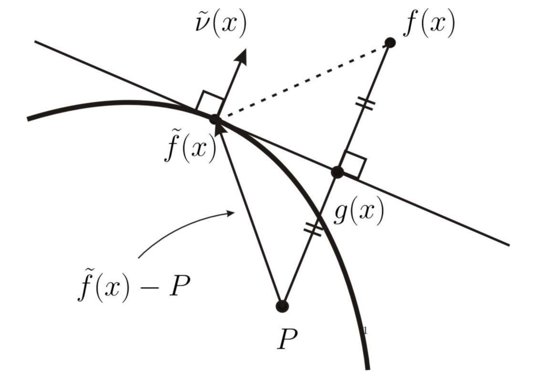 Figure 1
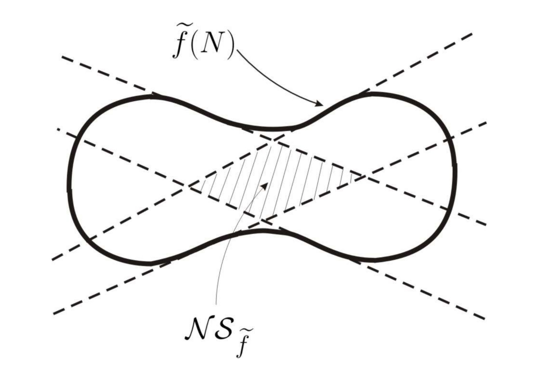 Figure 2
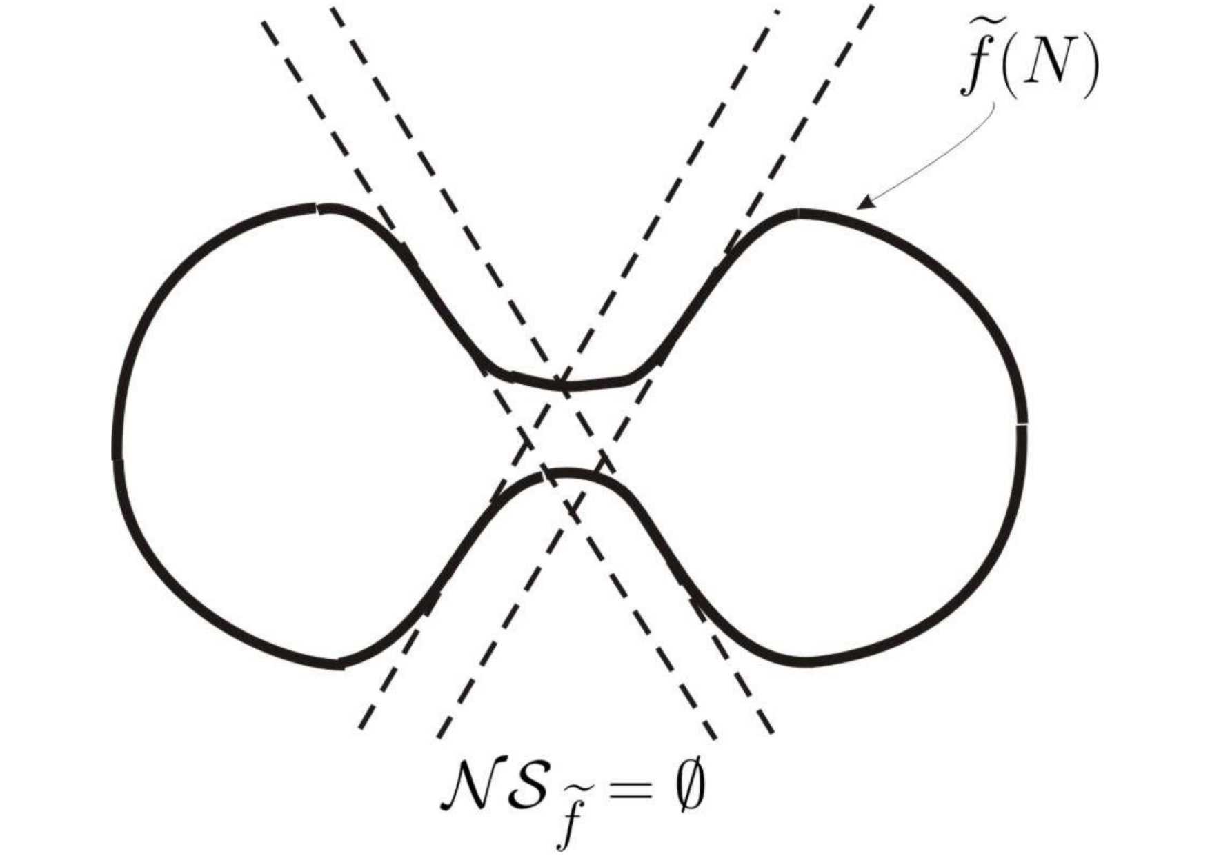 Figure 3
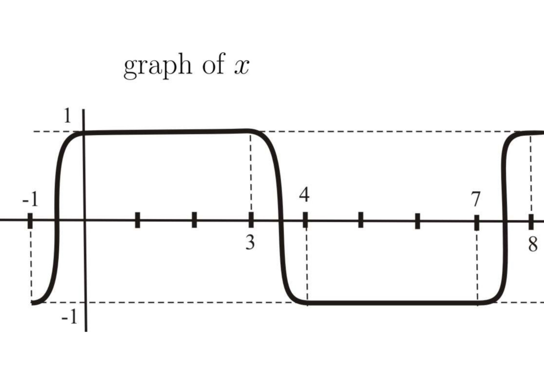 Figure 4
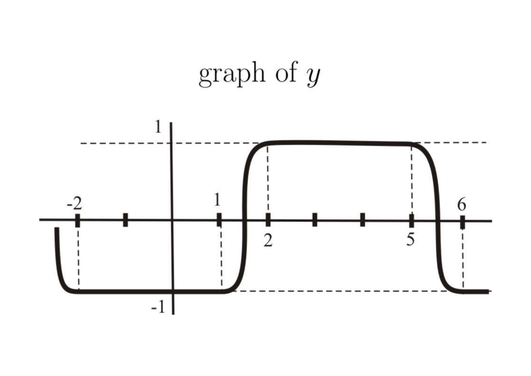 Figure 5
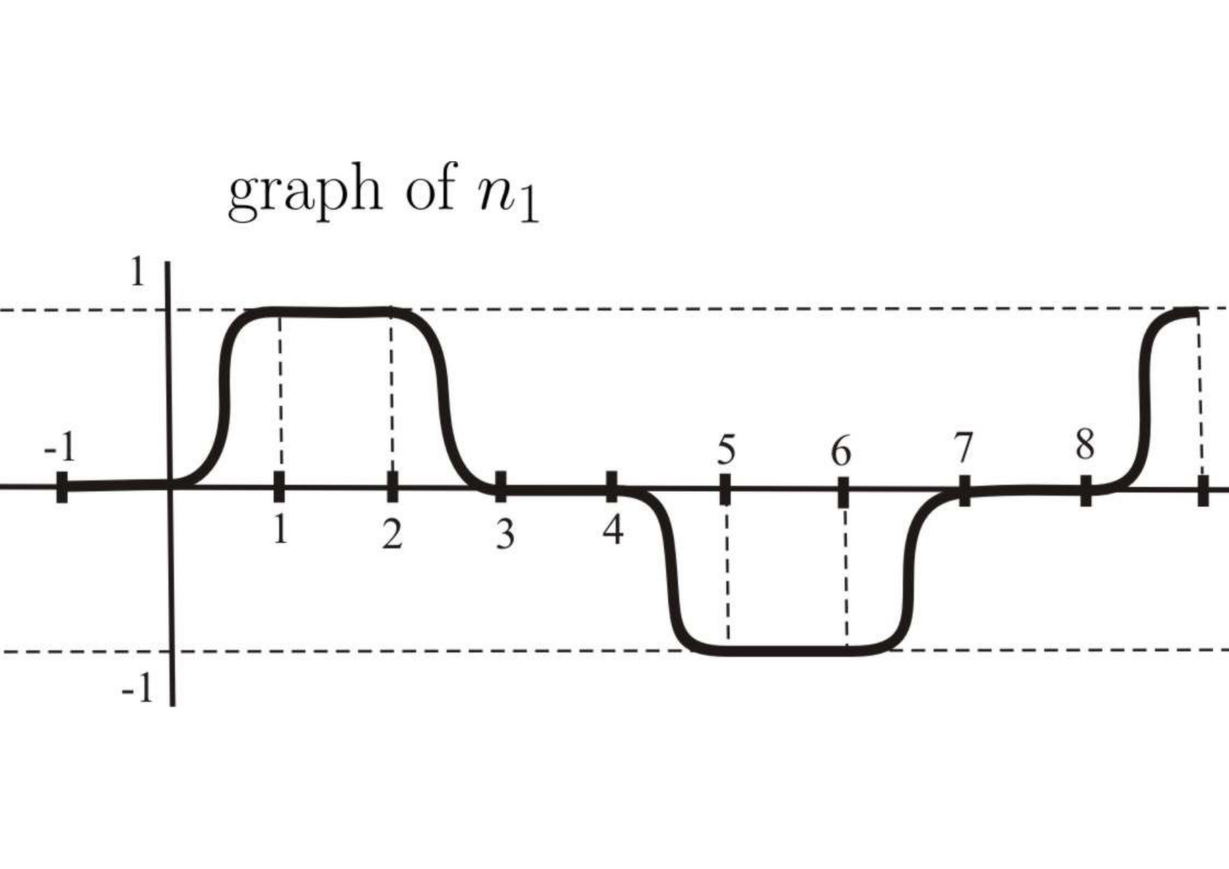 Figure 6
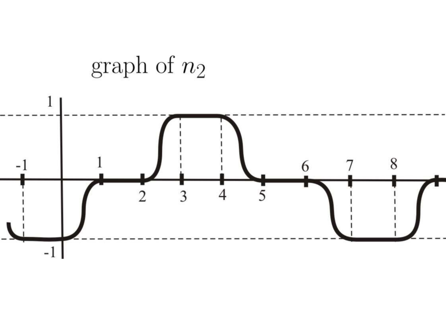 Figure 7
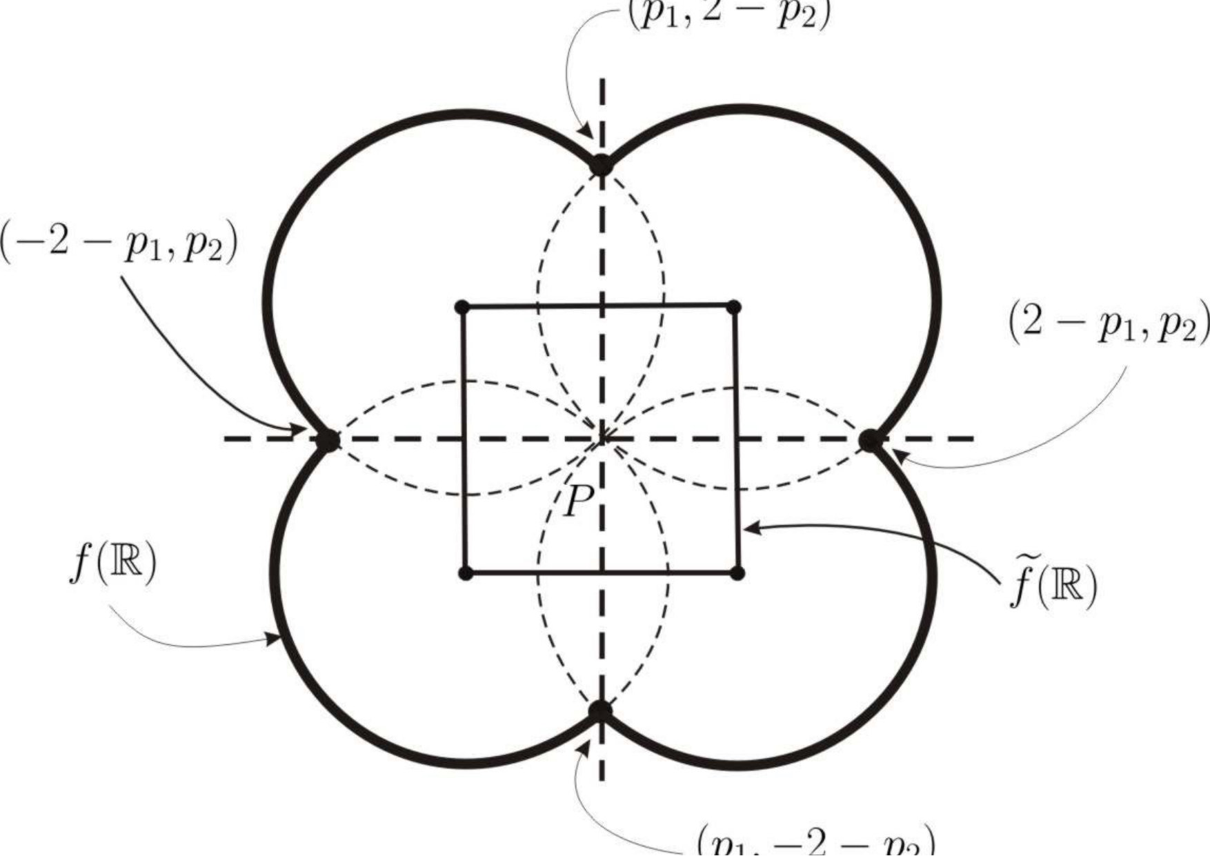 Figure 8
Peer Reviews
No public reviews on file for this paper yet. If you reviewed it on a platform where reviews are public (OpenReview, ICLR, NeurIPS, ICML), you can paste yours below so the community can read it here.
Videos
No videos yet. Explain this paper in a talk, walkthrough, or lecture? Add one.
Taxonomy
TopicsPoint processes and geometric inequalities · Analytic and geometric function theory · Geometric Analysis and Curvature Flows
Anti-orthotomics of frontals
and their applications
Stanisław Janeczko
Institute of Mathematics, Polish Academy of Sciences, ul. Sniadeckich 8, 00-956 Warsaw, POLAND
and
Faculty of Mathematics and Information Science, Warsaw University of Technology, ul. Koszykowa 75, 00-662 Warsaw, POLAND
and
Takashi Nishimura
Research Institute of Environment and Information Sciences, Yokohama National University, 240-8501 Yokohama, JAPAN
Abstract.
Let be a frontal with its Gauss mapping and let be a point such that for any . In this paper, for the mapping defined by
[TABLE]
the following four are shown. (1) is a frontal with its Gauss mapping at . (2) is the unique anti-orthotomic of relative to . (3) The property holds for any . (4) The equality holds for any .
Moreover, three applications of the main result are given. As the first application, a generalization of Cahn-Hoffman vector formula is given. The second application is to clarify an optical meaning of anti-orthotomics. The third application gives a criterion to be a front for a given frontal.
Key words and phrases:
Frontal, Anti-orthotomic, Orthotomic, Gauss mapping, Negative pedal, Pedal, No-silhouette condition, Cahn-Hoffman vector formula, Opening, Front, Variability condition, Proper frontal.
2010 Mathematics Subject Classification:
57R45, 58C25, 53A40
1. Introduction
Throughout this paper, let , be a positive integer and an -dimensional manifold without boundary respectively. Moreover, all mappings in this paper are of class unless otherwise stated.
A mapping is called a frontal if there exists a mapping such that the following two conditions are satisfied, where the dot in the center stands for the scalar product of two vectors in and two vector spaces and are identified:
- (1)
, i.e. for any . 2. (2)
for any and any .
By the above conditions and , it is natural to call the Gauss mapping of . In this paper, sometimes, even the mapping is called a frontal. The notion of frontal was independently introduced in several literature (e.g. [6, 12, 23, 27]) and it has been rapidly and intensively investigated (see [14]).
Definition 1**.**
Let be a frontal with its Gauss mapping and let be a point of .
- (1)
A mapping is called the orthotomic of relative to if the following equality holds for any .
[TABLE] 2. (2)
A mapping is called the pedal of relative to if the following equality holds for any .
[TABLE]
Figure 1 clearly illustrates the relation between the orthotomic and the pedal of relative to . The following Proposition 1 guarantees that the orthotomic of a given frontal is a frontal.
Proposition 1**.**
Let be a frontal and let be a point of such that the following condition is satisfied for any .
[TABLE]
Then, the orthotomic of relative to defined by
[TABLE]
is a frontal with its Gauss mapping . Moreover, the condition
[TABLE]
holds for any .
Proposition 1 will be proved in Section 2. By definition, it is clear that for the pedal , is the orthotomic. Thus, it is clear that Proposition 1 yields the following corollary which is a generalization of [18].
Corollary 1**.**
Let be a frontal and let be a point of such that the following condition is satisfied for any .
[TABLE]
Then, the pedal of relative to defined by
[TABLE]
is a frontal with its Gauss mapping . Moreover, the condition
[TABLE]
holds for any .
Notice that in the case that is a plane regular curve, it is well-known that is a normal vector to at (for instance, see [4]). Therefore, a part of Proposition 1 may be regarded as just a generalization of the classical result to frontals of general dimension.
Notice also that even if is non-singular, the condition “ for any ” seems not so mild. In other words, even when is an embedding, if the image of Gaussian curvature function of is a large interval containing zero as an interior point, then there are no points satisfying the condition “ for any ”. On the other hand, if is an embedding and the Gaussian curvature of is always positive, then the set is a non-empty open set. Moreover, the assumption “ is an embedding and the Gaussian curvature of is always positive” seems to be common for the study of orthotomics and pedals. (for instance, see [1, 5]). Therefore, the assumption given in Proposition 1 generalizes the common assumption for the study of orthotomics and pedals.
The same condition as the assumption of Proposition 1 has been already introduced by J. W. Bruce and P. J. Giblin in [4] 7.14 in the case that is regular; and also
by the second author ([21] in the case that is an immersion, [22] in the case that is a Legendrian map and [16] in the case that and is an embedding). Namely, in [16] the following set, called no-silhouette of and denoted by , is defined.
[TABLE]
For a frontal with its Gauss mapping , the notion of no-silhouette can be naturally generalized as follows. The optical meaning of no-silhouette is illustrated by Figure 2.
[TABLE]
Definition 2**.**
- (1)
Let be a mapping and let be a point of . A frontal with its Gauss mapping is called the anti-orthotomic of relative to if the following equality holds for any .
[TABLE] 2. (2)
Let be a mapping and let be a point of . A frontal with its Gauss mapping is called the negative pedal of relative to if the following equality holds for any .
[TABLE]
By definition, if , then the anti-orthotomic of relative to is exactly the same as the negative pedal of relative to . Depending on situations, sometimes, the negative pedal is also called the primitive (for example, see [2]) or the Cahn-Hoffman map (for instance, see [10, 15, 17]). In Geometric Optics, the notions of anti-orthotomic is very important (for example, see [1, 4, 5]), and for the study of Wulff shape, the notion of negative pedal is the core concept (for instance, see [7, 15, 17, 19, 26]).
By definition, it is clear that an anti-orthotomic (resp., a negative pedal) is a solution frontal for a given orthotomic equation (resp., pedal equation). Therefore, obtaining anti-orthotomics or negative pedals may be considered as inverse problems. It seems that, except for the case that the Gauss mapping of is non-singular (i.e. the case that is an embedding and the Gaussian curvature of is always positive), such inverse problems have been usually investigated only by solving simultaneous function equations for the envelopes.
Example 1**.**
Let be the mapping defined by . Define by . Then, is a frontal. Set and . Then, clearly, is the negative pedal of relative to and .
On the other hand, the function given by
[TABLE]
defines the one-parameter family of affine tangent lines to . And the solution figure of the simultaneous equation is .
Example 2**.**
Let be a periodic function of period satisfying the following condition for any .
[TABLE]
Let be a periodic function of period satisfying the following condition for any integer .
[TABLE]
Define by . Then, is a periodic mapping of period and the set of singular points of contains infinitely many closed intervals
[TABLE]
From Figure 3, it is clear that even if has other singular points, the image of is always the square with the following vertexes
[TABLE]
Next, in order to assert that is a frontal, we construct a non-zero normal vector ({\color[rgb]{0,0,0}\definecolor[named]{pgfstrokecolor}{rgb}{0,0,0}\pgfsys@color@gray@stroke{0}\pgfsys@color@gray@fill{0}n_{1}}(t),{\color[rgb]{0,0,0}\definecolor[named]{pgfstrokecolor}{rgb}{0,0,0}\pgfsys@color@gray@stroke{0}\pgfsys@color@gray@fill{0}n_{2}}(t)) to at . Let {\color[rgb]{0,0,0}\definecolor[named]{pgfstrokecolor}{rgb}{0,0,0}\pgfsys@color@gray@stroke{0}\pgfsys@color@gray@fill{0}n_{1}}:\mathbb{R}\to\mathbb{R} be a periodic function of period satisfying the following condition for any integer .
[TABLE]
Let {\color[rgb]{0,0,0}\definecolor[named]{pgfstrokecolor}{rgb}{0,0,0}\pgfsys@color@gray@stroke{0}\pgfsys@color@gray@fill{0}n_{2}}:\mathbb{R}\to\mathbb{R} be a periodic function of period satisfying the following condition for any integer .
[TABLE]
From Figure 3 and Figure 4, it is easily seen that the following two properties hold for any .
[TABLE]
Set
[TABLE]
Then, is actually a frontal.
For the frontal , the envelope of the one-parameter family of lines perpendicular to the unit vector and passing through the point does not restore the square .
These two examples show that, for frontals, the classical notion of envelope cannot restore the original figure in general. In order to eliminate the influence of singularities of frontals, Masatomo Takahashi has succeeded to improve the notion of envelopes ([24, 25]). The improvement due to Takahashi is nice, and thus for Example 1, the original figure can be actually obtained as the envelope of Takahashi’s sense. However, unfortunately, the variability condition defined in [24, 25] is not satisfied for the frontal given in Example 2. Thus, even Takahashi’s envelope cannot restore the original square of Example 2. In Ishikawa’s words, a frontal satisfying Takahashi’s variability condition is called a proper frontal ([14], §6). The frontal of Example 2 is not a proper frontal. To the best of authors’ knowledge, except for Example 2.5 given in [14], all frontals investigated in detail so far are proper frontals. We would like to assert that non-proper frontals, too, are useful especially in application to surface science (see §5).
The following Example 3 shows that the uniqueness of anti-orthotomic (resp., negative pedal) does not hold in general even when the given mapping (resp., ) is a frontal.
Example 3**.**
Let be the constant mappings defined by , . Let be the constant mapping defined by . Set and define the constant mapping by . Then, for any mapping with the form , the frontal is an anti-orthotomic of relative to and a negative pedal of relative to .
The main purpose of this paper is to obtain the unique solution of the inverse problem for a given orthotomic relative to such that .
Theorem 1**.**
Let , be a frontal and a point of such that respectively. Let be the mapping defined by
[TABLE]
Then, the following four holds:
- (1)
The mapping is a frontal with its Gauss mapping . 2. (2)
The mapping is the unique anti-orthotomic of relative to . 3. (3)
The point belongs to . 4. (4)
*The equality holds for any . *
In the case that and is a regular curve such that for any , the same formula for has been already given in [4] 7.14 as the envelope of perpendicular bysectors of segments joining and . On the other hand, by Proposition 1, must be in the normal line . Therefore, in Theorem 1, just by solving simultaneous linear equations, the same formula for can be obtained easily as the intersections of the perpendicular bysectors and the normal lines; and the no-silhouette condition guarantees that each simultaneous linear equation must have the unique solution.
The following corollary clearly follows from Theorem 1
Corollary 2**.**
Let , be a frontal and a point of such that respectively. Let be the mapping defined by
[TABLE]
Then, the following four holds:
- (1)
The mapping is a frontal with its Gauss mapping . 2. (2)
The mapping is the unique negative pedal of relative to . 3. (3)
The point belongs to . 4. (4)
*The equality holds for any . *
This paper is organized as follows. In Section 2, Proposition 1 is proved. Theorem 1 is proved in Section 3. In the case that the Gauss mapping of is the identity mapping, there is the famous Cahn-Hoffman vector formula for ([9]). In Section 4, as the first application of Theorem 1, Cahn-Hoffman formula is shown. In Section 5, as the second application of Theorem 1, the optical meaning of the anti-orthotomic is clarified even at a singular point of the Gauss mapping of . Moreover, in order to show how the clarified optical meaning is useful, it is applied to construct the exact shape of the orthotomic for the frontal in Example 2 and a given point . Finally, in Section 6, as the third application of Theorem 1, it is given a criterion that a given frontal is actually a front.
2. Proof of Proposition 1
2.1. Proof that is a frontal
with its Gauss mapping
Recall that is defined by .
Lemma 2.1**.**
For any , is a non-zero vector.
Proof.
Suppose that for some . Then, for the , the following holds:
[TABLE]
This implies which contradicts the assumption .
Set
[TABLE]
Then, it is sufficient to show that for any and any . In other words, it is sufficient to show that
[TABLE]
for any curve such that . The following lemma clearly holds:
Lemma 2.2**.**
- (1)
. 2. (2)
. 3. (3)
**
By using Lemma 2.2, we have the following:
[TABLE]
2.2. Proof that
for any
For any , we have the following:
[TABLE]
By the assumption , it follows that for any .
3. Proof of Theorem 1
3.1. Proof that is a frontal
with Gauss mapping
From the assumption that for any , it follows that for any . Thus,
[TABLE]
is well-defined. Then, it is sufficient to show that
[TABLE]
for any curve such that . Since has the form
[TABLE]
we have the following:
[TABLE]
3.2. Proof that is
the unique anti-orthotomic of relative to
The proof is essentially given in the paragraph next to Theorem 1. Thus, in this subsection, just a confirmation by definition is given.
Recall that . We have the following:
[TABLE]
3.3. Proof that
for any
For any we have the following:
[TABLE]
3.4. Proof that the equality
holds for any
Since , the following holds for any :
[TABLE]
4. Application 1:
Generalization of Cahn-Hoffman vector formula
Let be a frontal. We assume that is not empty. Let be a point of . Then, by Corollary 2, the mapping defined by
[TABLE]
is a frontal and the unique negative pedal of relative to . Set . Then, by using and , can be expressed as follows.
[TABLE]
In [9], under the assumption that is the unit sphere and is the identity mapping and under the identification , D. W. Hoffman and J. W. Cahn showed the following.
Theorem 2** (Cahn-Hoffman vector formula [9]).**
For any , the following equality holds.
[TABLE]
Here, stands for the gradient vector of at with respect to the normal coordinate system of around . In this section, as an application of Theorem 1, we generalize Theorem 2 as follows.
Theorem 3**.**
Let be a frontal and let be a point of . Suppose that is non-singular at . Then, the following equality holds.
[TABLE]
Here, stands for the transposed matrix of the inverse of Jacobian matrix of with respect to an arbitrary local coordinate system around and the normal coordinate system around . Theorem 3 yields not only Theorem 2 but also the following.
Corollary 3**.**
*Let be a frontal and let be a point of . Suppose that is non-singular at . Then, is a singular point of if and only if is satisfied. *
Proof of Theorem 3.
Since
[TABLE]
it follows
[TABLE]
where and .
In order to represent in terms of and , the same technique as in [20] is used. Since , for any ,
[TABLE]
where and . Thus, the Jacobian matrix of at with respect to an arbitrary local coordinate system around and the direct product of the normal coordinate system and around has the following form, where stands for the Jacobian matrix of at and stands for the transposed vector of the gradient of at .
[TABLE]
Let and be the cofactor matrix of the Jacobian matrix and the Jacobian determinant of at respectively. Moreover, let be the zero vector. Multiplying the matrix
[TABLE]
to the Jacobian matrix from the left side yields the following, where stands for the unit matrix.
[TABLE]
Hence we have the following.
Lemma 4.1**.**
Suppose that . Then, we may put as follows:
[TABLE]
Notice that in order to show that , the assumption “” is used .
Set . Then, by elementary geometry, we have
[TABLE]
Since , we have
[TABLE]
5. Application 2: Opening of Gauss mapping of
anti-orthotomic
The application in Section 4 is a result only at a non-singular point of . In this section, as the second application of Theorem 1, we investigate what can be asserted even at a singular point of . Several definitions are needed for the investigation of this section.
Definition 3** ([13]).**
Let be an equidimensional map-germ.
- (1)
Let denote the -module of -forms on . Then, the -module generated by in is called the Jacobi module of and is denoted by , where for a function-germ stands for the exterior differential of . 2. (2)
The ramification module of (denoted by ) is defined as the -module consisting of all function-germs such that belongs to .
Definition 4** ([13]).**
Let {\color[rgb]{0,0,0}\definecolor[named]{pgfstrokecolor}{rgb}{0,0,0}\pgfsys@color@gray@stroke{0}\pgfsys@color@gray@fill{0}\varphi}:(\mathbb{R}^{n},0)\to(\mathbb{R}^{n},0) be an equidimensional map-germ and let {\color[rgb]{0,0,0}\definecolor[named]{pgfstrokecolor}{rgb}{0,0,0}\pgfsys@color@gray@stroke{0}\pgfsys@color@gray@fill{0}\delta}:(\mathbb{R}^{n},0)\to(\mathbb{R},0) a function-germ. Then, the map-germ ({\color[rgb]{0,0,0}\definecolor[named]{pgfstrokecolor}{rgb}{0,0,0}\pgfsys@color@gray@stroke{0}\pgfsys@color@gray@fill{0}\varphi,\delta}):(\mathbb{R}^{n},0)\to(\mathbb{R}^{n}\times\mathbb{R},(0,0)) is called an opening of if .
Theorem 4**.**
Let be a frontal. Let and satisfy . Then, is an opening of the Gauss map-germ of its anti-orthotomic .
The optical meaning of anti-orthotomic is straightforward from Theorem 4. By definition, we have the following corollary.
Corollary 4**.**
Let be a frontal. Let and satisfy . Then, is an opening of the Gauss map-germ of its negative pedal .
Proof of Theorem 4.
Let be a sufficiently small open neighbourhood of and let be a normal coordinate system at . Let be a sufficiently small open neighbourhood of such that and set for any . Moreover, for any , set . Since is the Gauss mapping of and , we have
[TABLE]
Since , it follows . Thus, we have
[TABLE]
Consider again the frontal given in Example 2. Recall that the image is the square with vertexes . Let be a point such that . Then, belongs to . Let be the orthotomic of relative to . Theorems 1 and 4 reduce the construction of the image of to elementary geometry, which is explained as follows (see Figure 5).
By the construction of , if belongs to the union of closed intervals
[TABLE]
then must be a singular point of . Thus, by Theorem 4, must be a singular point of , and therefore each of must be one point. By definition, the one point must be the mirror image of as follows.
Lemma 5.1**.**
[TABLE]
By the construction of ,
[TABLE]
By the assertion (4) of Theorem 1, the following holds.
Lemma 5.2**.**
[TABLE]
By the construction of , we have the following.
Lemma 5.3**.**
- (1)
* is exactly the hemicircle centered at with boundary and which does not contain .* 2. (2)
* is exactly the hemicircle centered at with boundary and which does not contain .* 3. (3)
* is exactly the hemicircle centered at with boundary and which does not contain .* 4. (4)
* is exactly the hemicircle centered at with boundary and which does not contain .*
For the precise shape of the pedal of relative to , just shrink to percent with respect to .
It seems that the method of C. Herring explained in [8] is similar as our method. However, his method seems to rely on a thermodynamical consideration of atoms. Our method needs no physical consideration. Once the given shape is realized as the image of frontal , by applying Theorem 1 and Theorem 4, only elementary geometry is needed. In other words, under any physical situation, if the same square is given, then the -plot for the square must have the same shape.
6. Application 3: A criterion for fronts
Definition 5**.**
A germ of frontal is called a germ of front (or front-germ) if is non-singular at .
Given a frontal , if is a germ of front for any , then is called a front. A front is also called a wave-front. For details on fronts, see for example [2, 3].
Theorem 5**.**
Let be a frontal and let be a point of . Then, for any point such that , the following are equivalent, where is the anti-orthotomic germ of relative to .
- (1)
* is a front-germ.* 2. (2)
* is a front-germ.* 3. (3)
* is non-singular.*
Theorem 5 answers the question communicated by A. Honda and K. Teramoto ([11]). Theorem 5 yields the following corollaries.
Corollary 5**.**
Let be a frontal and let be a point of . Then, for any point such that , the following are equivalent, where is the negative pedal germ of relative to .
- (1)
* is a front-germ.* 2. (2)
* is a front-germ.* 3. (3)
* is non-singular.*
Corollary 6**.**
Let be a frontal. Let two points and satisfy . Let be the anti-orthotomic of relative to . If is not contained in SingSing, then the map-germ is a front-germ; where for a mapping , Sing stands for the singular set of . In particular, if is non-singular, then must be a front-germ.
Corollary 7**.**
Let be a frontal. Let two points and satisfy . Let be the negative pedal of relative to . If is not contained in SingSing, then the map-germ is a front-germ. In particular, if is non-singular, then must be a front-germ.
Corollary 8**.**
*Let be a frontal. Let two points and satisfy . Let be the orthotomic of relative to . If is not contained in SingSing, then the map-germ is a front-germ. *
Corollary 9**.**
*Let be a frontal. Let two points and satisfy . Let be the pedal of relative to . If is not contained in SingSing, then the map-germ is a front-germ. *
Proof of Theorem 5.
is just a corollary of Theorem 4. is trivial. Thus, in order to complete the proof, it is sufficient to show . Suppose that is non-singular. Then, is non-singular. By the assumption , it follows that the projection is injective. Therefore, is non-singular.
Acknowledgement
The authors thank Masatomo Takahashi for teaching them his improvement of classical envelope. The second author was supported by JSPS KAKENHI Grant Number 17K05245.
The reference list from the paper itself. Each links out to its DOI / PubMed record.
- 1[1] N. Alamo and C. Criado, Generalized antiorthotomics and singularities , Inverse Problems, 18 (2002), 881–889.
- 2[2] V. I. Arnol’d, Singularities of Caustics and Wavefronts , Mathematics and its Applications, 62 , Springer Netherland, Dordrecht, 1990.
- 3[3] V. I. Arnol’d, S. M. Gusein-Zade, and A. N. Varchenko, Singularities of Differentiable Maps I , Monographs in Mathematics 82 , Birkhäuser, Boston Basel Stuttgart, 1985.
- 4[4] J. W. Bruce and P. J. Giblin, Curves and Singularities (second edition) , Cambridge University Press, Cambridge, 1992.
- 5[5] J. W. Bruce, P. J. Giblin and C. G. Gibson, On caustics by reflection , Topology, 21 (1982), 179–199.
- 6[6] S. Fujimori, K. Saji, M. Umehara and K. Yamada, Singularities of maximal surfaces , Math. Z., 259 (2008), 827–848.
- 7[7] H. Han and T. Nishimura, Spherical method for studying Wulff shapes and related topics , Adv. Stud. Pure Math., 78 , 1–53, Math. Soc. Japan. Tokyo, 2018.
- 8[8] C. Herring, Some theorems on the free energies of crystal surfaces , Physical Review, 82 (1951), 87–93.