Expression of the peak time for time-domain boundary measurements in diffuse light
Junyong Eom, Manabu Machida, Gen Nakamura, Goro Nishimura, and, Chunlong Sun

TL;DR
This paper provides a mathematical analysis of the peak time in time-domain boundary measurements of diffusive media, establishing its properties and relation to object position, with implications for optical imaging.
Contribution
It offers the first rigorous proof of existence, uniqueness, and explicit expression of the peak time in diffusive media, linking it to object location.
Findings
Proved existence and uniqueness of the peak time.
Derived explicit expression for the peak time.
Established relationship between peak time and object position.
Abstract
Light propagation through diffusive media can be described by the diffusion equation in a space-time domain. Further, fluorescence can be described by a system of coupled diffusion equations. This paper analyzes time-domain measurements, which measure the temporal point-spread function (TPSF), at a boundary of such diffusive media with a given source and detector. We focus on the temporal position of the TPSF maximum, which we refer to as the peak time. Although some unique properties of solutions of this system have been numerically studied, we give a mathematical analysis of peak time, providing proof of the existence, uniqueness, and the explicit expression of the peak time. We clearly show the relationship between the peak time and the object position in a medium.
Click any figure to enlarge with its caption.
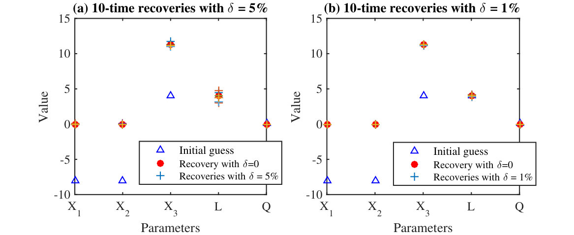 Figure 10
 Figure 11
 Figure 12
 Figure 13
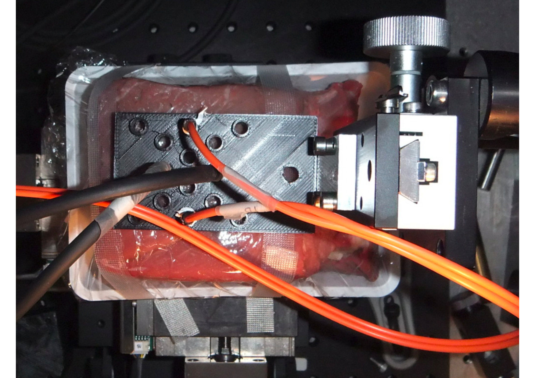 Figure 13
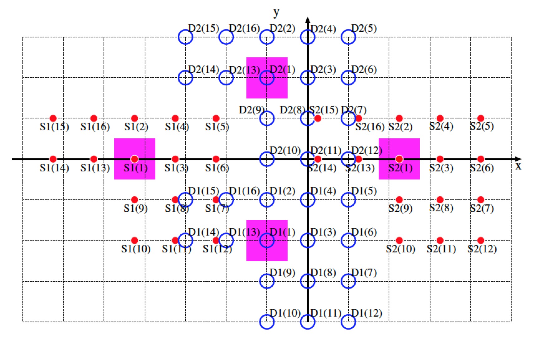 Figure 14
 Figure 15
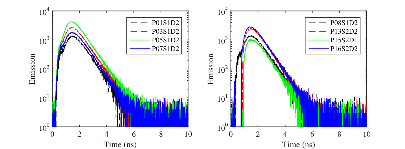 Figure 16
 Figure 17
 Figure 18
 Figure 1
 Figure 1
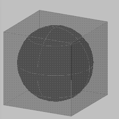 Figure 1
 Figure 2
 Figure 3
 Figure 4
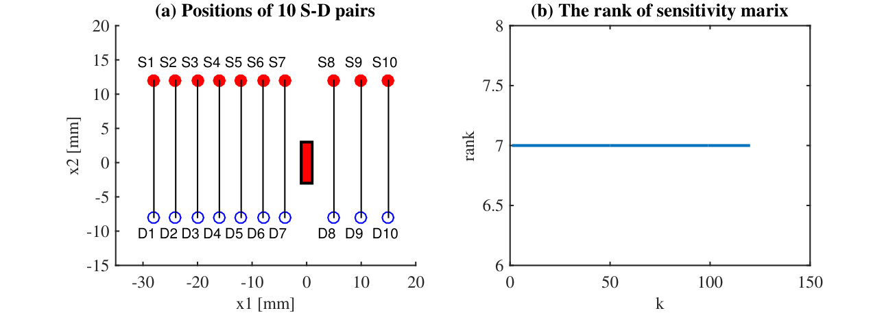 Figure 5
 Figure 6
 Figure 7
 Figure 8
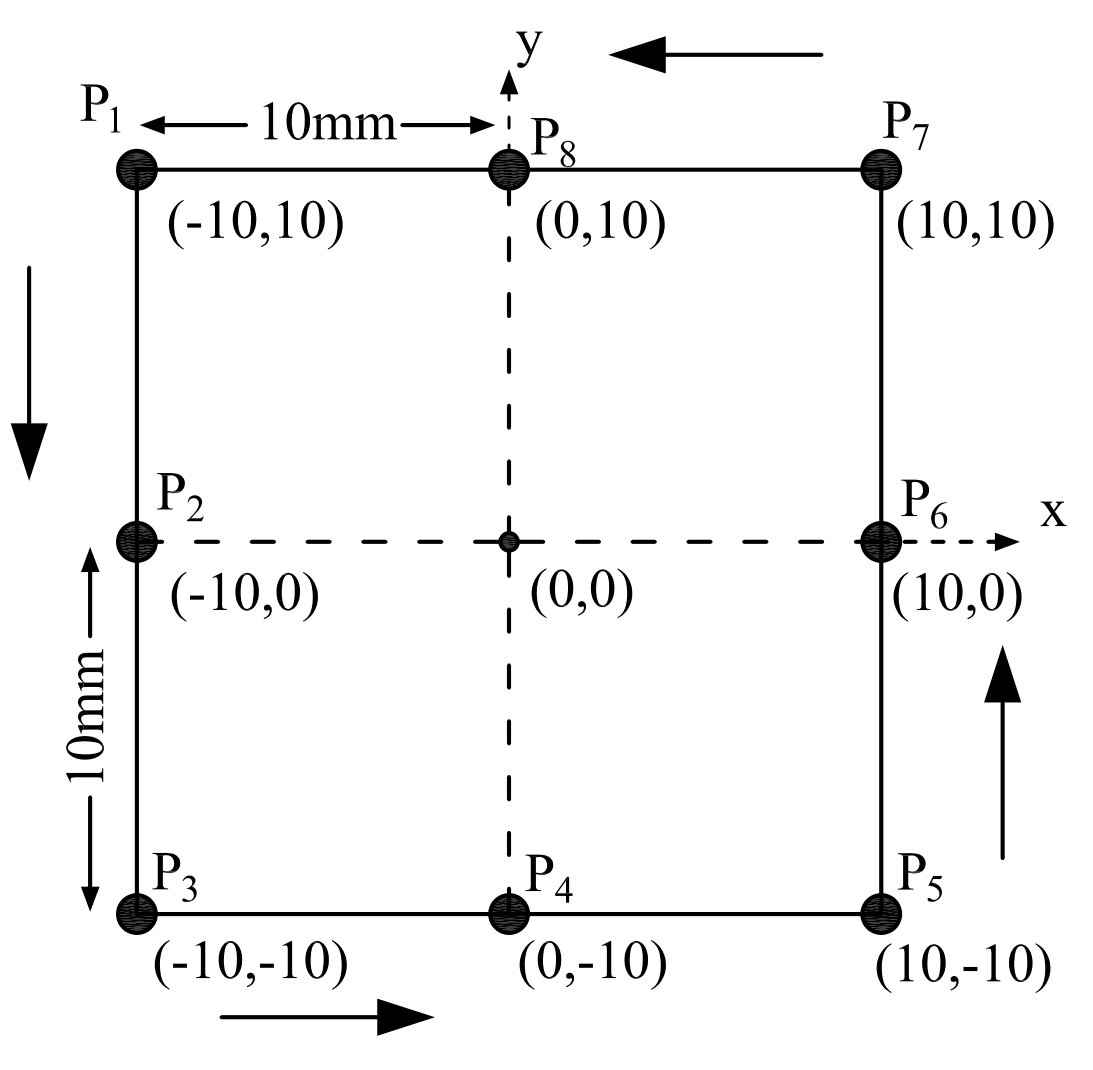 Figure 8
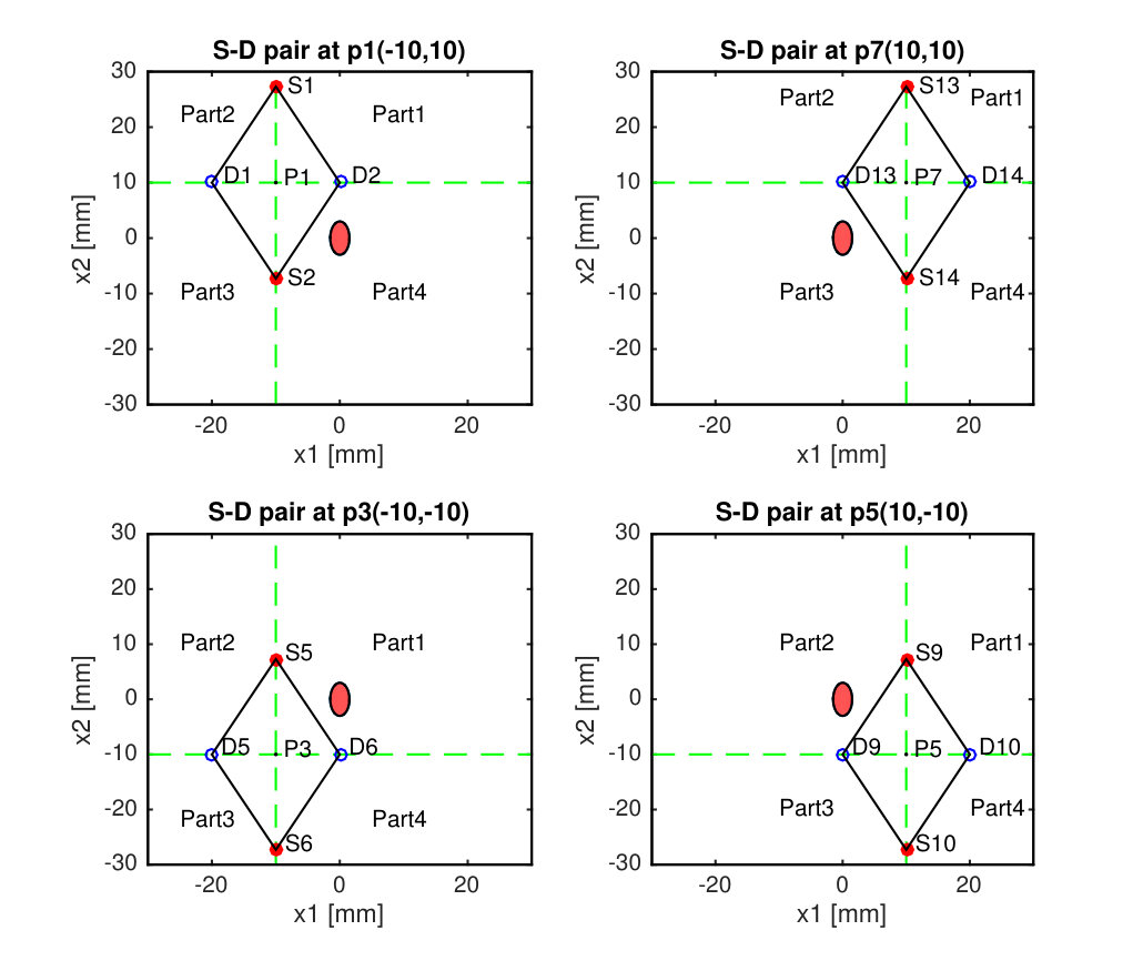 Figure 9
Peer Reviews
No public reviews on file for this paper yet. If you reviewed it on a platform where reviews are public (OpenReview, ICLR, NeurIPS, ICML), you can paste yours below so the community can read it here.
Videos
No videos yet. Explain this paper in a talk, walkthrough, or lecture? Add one.
Taxonomy
TopicsOptical Imaging and Spectroscopy Techniques · Advanced Fluorescence Microscopy Techniques · Photochemistry and Electron Transfer Studies
Expression of the peak time for time-domain boundary measurements in diffuse light
J.Y. Eom
Graduate School of Mathematical Sciences, The University of Tokyo, Tokyo 153-8914, Japan
M. Machida
Institute for Medical Photonics Research, Hamamatsu University School of Medicine,
Hamamatsu 431-3192, Japan
G. Nakamura
Department of Mathematics, Hokkaido University, Sapporo 060-0810, Japan and Research Center of Mathematics for Social Creativity, Research Institute for Electronic Science, Hokkaido University, Sapporo, 060-0811, Japan
G. Nishimura
Research Institute for Electronic Science, Hokkaido University, Sapporo 001-0020, Japan
C.L. Sun
College of Science, Nanjing University of Aeronautics and Astronautics, Nanjing 211106, P.R. China
Nanjing Center for Applied Mathematics, Nanjing 211135, P.R.China.
Abstract
Light propagation through diffusive media can be described by the diffusion equation in a space-time domain. Further, fluorescence can be described by a system of coupled diffusion equations. This paper analyzes time-domain measurements, which measure the temporal point-spread function (TPSF), at a boundary of such diffusive media with a given source and detector. We focus on the temporal position of the TPSF maximum, which we refer to as the peak time. Although some unique properties of solutions of this system have been numerically studied, we give a mathematical analysis of peak time, providing proof of the existence, uniqueness, and the explicit expression of the peak time. We clearly show the relationship between the peak time and the object position in a medium.
††preprint: AIP/123-QED
I Introduction
Light propagation in highly scattering medium, such as biological tissue, is dominated by multiple scattering. The propagation can be described by an initial-boundary value problem for a diffusion equation in a space-time domain given as
[TABLE]
where represents the specified background medium with boundary , is the photon density of light, is the unit outward normal, is the speed of light in the medium, is the photon diffusion coefficient and is the absorption coefficient of mediumMarttelli ; Jiang11 ; Durduran10 . Here is the location of point source and is a parameter given by
[TABLE]
with the Fresnel reflectance , which depends on the refractive index ratio between the medium and the free space Marttelli .
The initial-boundary value problem (1) is usually used for the light propagation in highly scattering media, such as biological tissues and is applied for the quantitative analysis of the optical properties of the mediumMycek03 ; Rudin13 ; Nitziachristos V02 ; Arridge99 ; Arr09 . This kind of analysis is so-called diffuse optical spectroscopy (DOS) or more sophisticated one, diffuse optical tomography (DOT). The DOS or DOT is to identify the unknown absorption coefficient and diffusion coefficient from the time-domain (TD) measurements at the boundary
[TABLE]
which depend on both of the space and time.
On the other hand, fluorescence in highly scattering medium is also very important in the applications and can be quantified by a similar initial-boundary value problem. In case of the fluorescence, two physical processes are coupled, namely excitation and fluorescence (emission). First, the excitation light injected from the boundary propagate in the medium as (1) and then absorbed by the fluorophores. Next, fluorescence emitted from the fluorophores propagate in the medium and is finally detected by a detector on the boundary described by
[TABLE]
In general, and here are not the same as the excitation ones in (1). We assume these are the same in this paper, corresponding to a case when the excitation and emission wavelengths are close and . The source term for on the right-hand side of (3) contains the excitation field and is specified by
[TABLE]
where is the fluorescence lifetime and is the absorption coefficient of fluorophores. Here we assume the optical parameters for fluorescence are same to those for the excitation and the absorption of the fluorophores is sufficiently smaller than the absorption of the medium. The inverse problem to identify the unknown absorption coefficient from the TD boundary measurements
[TABLE]
is referred to as the TD fluorescence diffuse optical tomography (FDOT)Lam05 ; Han08 ; Gao08 .
For above inverse problems of DOS and FDOT, other two types of the measurements, continuous wave (CW) Patwardhan05 ; Ducros11 and frequency domain (FD) Nitziachristos01 ; Corlu-etal07 ; Milstein04 , are also used. Among above three types of measurements, the TD measurements measure the temporal point-spread function (TPSF) and will provide the most fruitful information. Even though this advantage, it is believed that the effective choice of TPSF data is needed to extract important information about the unknown target. The possible choices of the TPSF data and the relative robustness of the different sets of data to noise are considered J.Riley07 . They refer the data in the whole TPSF as global data types, whereas the types of information only local to the high signal area are referred to local data types. It was examined that the local data types are more robust to noise than global data types, and should provide enhanced information to the related inverse problems.
In this paper, we denote the temporal position of the maximum of TPSF as peak time and assume . One has demonstrated direct depth estimation of a localized fluorescent object from the peak time by numerical experimentsD. Hall04 . The depth estimation permits recovery of the fluorophore concentration, which is a robust and efficient approach since the peak time is independent of the fluorophore concentration. However, the rigorous mathematical analysis of the peak time has not been provided yet as far as we know. In case of , one can find an explicit expression of the peak time of TD boundary measurements (2) but for the Direchlet boundary condition case ()G.Nishi05 . We will give the explicit expressions of peak time for the TD boundary measurements (2) and (5), by which we can construct the connection between the peak time and unknown important information in the related inverse problems.
A mathematically well known hot spots problem is to extract which spatial point is the hottest point Siudeja15 ; Rodrigo99 ; Burdzy99 , whereas the peak time problem in this paper is to extract the time point at which the photon density of TD boundary measurements is strongest. Both of them are the problems of studying the evolution of solution’s maximum value. Searching general schemes to identify a profile with peaks for convolutions of functions has been studied in signal processing Vidmar03 ; Shensa92 ; lin06 . For instance, there is a scheme using continuous wavelet transformslin06 . We tried in this paper to derive the peak time by using an asymptotic analysis.
The rest of this paper is organized as follows. In section II, under some simple assumptions, we show the asymptotic behavior of TD boundary measurements. Section III shows the explicit expressions of the peak time for the boundary excitation measurements (2) and the boundary emission measurements (5), respectively. The unique existence of peak time is also considered in this section. Finally, section IV is devoted to conclusion and remark.
II Asymptotic behavior of the boundary measurements
In the measurement setup of DOT or FDOT, the source and detection optical fibers are placed on the boundary surface . We are here considering measurements, which are a set of source and detector pair on the same surface of biological tissue, and the distance between source and detector is very small rather than the tissue size. In this case, we can assume the half space for the modeling of tissue. Hence we can model as
[TABLE]
with the boundary . On the other hand, we assume that the absorption coefficient and the diffusion coefficient are constants everywhere in the medium. In this paper we consider the zero-lifetime case of model (3), i.e., the lifetime in the source term is . Furthermore, we assume the size of fluorescence target in (3) is very small such that it can be approximated by
[TABLE]
where is the location of point target.
Under above assumptions, we are going to obtain the analytical expressions of excitation light and zero-lifetime emission light. Let be the Green function, which satisfies
[TABLE]
for a given point source located at . One can obtain the analytical expression of by the functional solution of heat equation Haskell , which has been investigated extensively in the scientific community. That is
[TABLE]
where
[TABLE]
with the complementary error function
[TABLE]
Then, by the general theory of partial differential equations, we have the following expression for as
[TABLE]
Next, we consider the analytical solution of zero-lifetime emission light. Let be the photon density of zero-lifetime emission light. For , integrating (4) by parts with respect to gives
[TABLE]
Since ,
[TABLE]
due to (8). This implies that for each fixed , is bounded with respect to . Hence there exists a constant depending on such that
[TABLE]
for . Together with this and , we immediately have for that
[TABLE]
Hence the photon density of zero-lifetime emission light satisfies the following initial-boundary value problem
[TABLE]
which implies the solution to initial-boundary value problem (3) is the convolution of zero-lifetime emission with the lifetime function , i.e.,
[TABLE]
Now, by using the Green function and the expression of as in (8), we have the following analytical expression for as
[TABLE]
In particular, for any given , we have by (7), (8) and (10) that
[TABLE]
and
[TABLE]
where
[TABLE]
In what follows, if there is no specification, we will define
[TABLE]
where is the Euclidean norm of any three dimensional vector . Then, by (13), we can write of (12) as
[TABLE]
where
[TABLE]
with
[TABLE]
for . We will consider the peak time for (14). More precisely, we will consider the explicit expressions of approximate peak time for (14) in three cases where in the boundary condition is really small, large and general value, respectively. This implies that we need to construct the connections between (14) with the TD boundary measurements corresponding to Neumann boundary condition and Dirichlet boundary condition, respectively. We do that by analyzing the asymptotic behavior of TD boundary measurements for as follows.
Lemma 1
Corresponding to the case of , we set
[TABLE]
which is the boundary measurements of (9) corresponding to Neumann boundary condition. Then, there holds the following asymptotic behavior
[TABLE]
Proof: By applying the integration by parts for the complementary error function, we have
[TABLE]
and
[TABLE]
for . This together with (16) implies
[TABLE]
for , where . Then by (15) we obtain
[TABLE]
for . Similarly we have for .
Note the definition of as in (17). By (14), (17) and (19), we obtain the estimation
[TABLE]
for , implying the asymptotic behavior as in (18).
The proof is complete.
Lemma 2
Corresponding to the case of , we set
[TABLE]
which is the boundary measurements of (9) corresponding to the Dirichlet boundary condition. Then, there holds the following asymptotic behavior
[TABLE]
Proof: Since
[TABLE]
this together with (16) implies
[TABLE]
for , where is independent of and . Here constants may have different values also within the same line. We remark as . Then by (15)
[TABLE]
and
[TABLE]
for . Then this together with (14), (20) and (II) implies that
[TABLE]
as .
Since
[TABLE]
we obtain
[TABLE]
where is as in (20). The proof is complete.
III The peak time of boundary measurements
In this section, we will show the expressions of the approximate peak time for TD boundary measurements (11) and (14), respectively.
III.1 The expression of peak time for
We consider the expression of peak time for TD boundary measurements as in (11). Likewise Lemma 1, we first investigate the asymptotic behavior of in the following two limiting cases:
[TABLE]
and
[TABLE]
Then, based on the asymptotic expansion of , we are able to present the expression of the approximate peak time for . By the expression of as in (11), we have
[TABLE]
where
[TABLE]
and
[TABLE]
with . We have the asymptotic behavior for that
[TABLE]
as , and
[TABLE]
as . Now we are ready to give the expression of approximate peak time of as follows.
Theorem 3
(1) If , the TD boundary measurements uniquely attains the maximum approximately at
[TABLE]
(2) If , then uniquely attains the maximum approximately at
[TABLE]
Proof: Since
[TABLE]
we obtain
[TABLE]
by using (24) and (25). This together with the expression of the derivative of
[TABLE]
implies that
[TABLE]
Finally, computing yields that attains the maximum approximately at as in (26) and (27) with respect to the cases and . Further, it is clear that the peak time is unique.
The proof is complete.
III.2 The Neumann boundary condition
We consider the Neumann boundary condition, i.e., in (1) and (9). Then we investigate the peak time for TD boundary measurements (i.e., as in (17)). We first consider the existence of peak time for , which is to prove that there exists one time point such that . The precise statement is given by the following theorem.
Theorem 4
There exist such that
[TABLE]
and
[TABLE]
Proof: Observe that
[TABLE]
Then we have
[TABLE]
for , where , are as in (15) and
[TABLE]
for . Then we have for that
[TABLE]
for , where is the positive solution of
[TABLE]
That is
[TABLE]
Let is the positive solution of
[TABLE]
We take . Then by (32) we have
[TABLE]
implying (28) is established.
On the other hand, for , we have
[TABLE]
for . This implies
[TABLE]
for . Since
[TABLE]
with for , we obtain
[TABLE]
for .
Set
[TABLE]
with . Then by (32), (34) and (35) we have
[TABLE]
implying (29) is established. The proof is complete.
In Theorem 4, we only proved the existence of peak time of for general and , without giving its uniqueness. However, for the case of , we are able to show the uniqueness of peak time and present its explicit formula.
Theorem 5
Suppose . Then there holds
[TABLE]
where and are as in (13). Further, admits the unique peak time
[TABLE]
Proof: By (31), we have
[TABLE]
where
[TABLE]
Since , it is easy to see that
[TABLE]
By the change of variable , there holds
[TABLE]
We transform the integration variable to which transforms to , and is given as \sigma=\big{(}1-\sqrt{1-4z^{-1}}\big{)}/2. Then, further transforming to , which yields the following
[TABLE]
By straight computation, we have
[TABLE]
This together with (III.2) implies
[TABLE]
and
[TABLE]
Then, by computing we can see that attains the maximum at the time as in (38).
The proof is complete.
We next consider the peak time of for the case but is small enough. Set
[TABLE]
We will prove as and give the expression of approximate peak time for with respect to the case is very small, which is stated as the following theorem.
Theorem 6
Let and be as in (17) and (41), respectively. Then
[TABLE]
Further, if , the peak time of can be approximated by
[TABLE]
Proof: By denoting and a transformation of integration variable for (39) and (40), we have
[TABLE]
Note that
[TABLE]
and
[TABLE]
Now we are ready to show the asymptotic behavior as in (42). By the mean value theorem for between and , there exists such that
[TABLE]
for . This together with (44) implies
[TABLE]
Similarly, we have the estimation for that
[TABLE]
Then, by (46) and (47) we immediately have the estimation
[TABLE]
implying that
[TABLE]
as . By the expression of as in (41), we obtain
[TABLE]
Finally, by computing we can see that attains the maximum at the time as in (43).
The proof is complete.
Remark 7
Based on the asymptotic behavior of in above Lemma 1, the peak time of as in (14) can be approximated by (43) if and .
III.3 The Dirichlet boundary condition
Here we consider the Dirichlet boundary condition, i.e., in (1) and (9). Then we study the peak time of TD boundary measurements (i.e., as in (20)). By the similar arguments as in Theorem 5 and Theorem 6, we will show the expression of peak time for .
Theorem 8
Suppose . Then there holds
[TABLE]
where and are as in (13). Further, admits unique peak time
[TABLE]
where
[TABLE]
and
[TABLE]
with .
Proof: By (20), we have
[TABLE]
where
[TABLE]
Likewise Theorem 5, we have by that
[TABLE]
This together with (50) implies (48) and
[TABLE]
Then, by computing we can see that attains the maximum at the time as in (49), i.e., (49) is the unique positive zero of the following cubic polynomial given as
[TABLE]
because for . Then the proof is complete.
Remark 9
If , by (48) we have
[TABLE]
This yields that admits unique approximate peak time
[TABLE]
under the condition .
We next consider the peak time of for the case but is small enough. Set
[TABLE]
Likewise Theorem 6, we can have the asymptotic behavior of . Then we arrive at the expression of peak time for under the condition is small enough. Since the same argument in Theorem 6 still works in our setting, we will state the following conclusion and omit the proof here.
Theorem 10
There holds
[TABLE]
Then, if but , the expression of peak time for can be approximately given as in (49) by replacing by .
We will give a remark before closing this subsection.
Remark 11
Together Remark 9, Theorem 10 with the asymptotic behavior of in Lemma 2, we can approximate the peak time of as in (14) by
[TABLE]
if provided that and .
III.4 The Robin boundary condition
Now we consider the Robin boundary condition, i.e., is a positive constant in (1) and (9). Then we consider the peak time for as in (14). We do that basically based on the asymptotic expansion of the complementary error function given as
[TABLE]
Lemma 12
Suppose
[TABLE]
and
[TABLE]
Then, there holds
[TABLE]
where and is given as (62).
Proof: With the assumption (59), we have the asymptotic expansion (58) for any . With the assumption (60), there holds
[TABLE]
Then, by (14), we can express as
[TABLE]
Here,
[TABLE]
By changing variables as , , and then , we arrive at
[TABLE]
where
[TABLE]
By straight computations, we have
[TABLE]
where
[TABLE]
We note that and . Thus,
[TABLE]
Therefore,
[TABLE]
The proof is complete.
Now we give the expression of approximate peak time for , which is stated as the following theorem.
Theorem 13
Suppose , and the conditions in Lemma 12 are established. Then, admits the approximate peak time
[TABLE]
Proof: By the assumptions
[TABLE]
we have
[TABLE]
Since is large, there holds . Then, at , by Lemma 12 we have
[TABLE]
Hence,
[TABLE]
By computing , we obtain
[TABLE]
which is the unique positive solution of following equation
[TABLE]
The proof is complete.
In Theorem 13, under some assumptions for physical parameters, we showed the expression of approximate time for TD boundary measurements with Robin boundary condition. Here we give a remark to show the limiting assumptions in above theorem are not strict in practice.
Remark 14
The assumption (59) can be achieved for typical physiological parameters. For example, we set
[TABLE]
which are typical values of biological tissues. Hereafter the unit of length is mm. In this case, there holds
[TABLE]
for . Further, if we set , and , the assumption can be satisfied. In this case, we have
[TABLE]
IV Conclusion and Remark
In this paper, we considered the TD boundary measurements, which means that the measured data for each given source and detector is a TPSF. One can expect that the TPSF corresponding to a single point target always admits a unique maximum from the physics intuition. We have mathematically investigated this physical phenomenon in this paper. By analyzing the asymptotic behavior of the TPSF, we proved the unique existence of the peak time for TD boundary measurements.
The peak time is an important property of TPSF. The local data types around the peak time are more robust to noise than other data types, and should provide enhanced information to the related inverse problems such as DOT and FDOTJ.Riley07 . Further, the recovery of unknown information from the measured data around peak time is a robust and efficient approachD. Hall04 . However, the explicit relations between the peak time and the unknowns have not been discussed yet. In this paper, we explicitly give an approximate expression of the peak time for both the boundary excitation measurements as in (11) and the boundary emission measurements as in (12). The expression of approximate peak time for clearly shows the relationship between the peak time and the important information of medium such as the absorption coefficient and the diffusion coefficient . The expression of approximate peak time for shows not only the dependence of peak time on but also the connection between the peak time and the position of an unknown point target. The above identities connecting the peak time of measurements and the unknowns in related inverse problems provide the possibility of constructing an effective and fast inversion scheme for the inverse problems. We will study the inverse problem of DOT and FDOT, and discuss an inversion scheme based on the explicit expression of the peak time in the forthcoming paper.
We remark that the expressions of peak time in this paper are obtained under some assumptions for the physical parameters and the object. We assume the size of fluorescence target is very small such that it can be approximated by the Dirac -function. However, we can still provide the prior information for general FDOT from the expression of peak time by assuming a point target.
Acknowledgements.
The first author was supported by JSPS KAKENHI (Grant No. JP20F20327). The third author was supported by JSPS KAKENHI (Grant No. JP19K03554). The fourth author was supported by JSPS KAKENHI (Grant No. JP19K04421). The last author was supported by National Natural Science Foundation of China (Grant No. 11971104) and by Natural Science Foundation of Jiangsu Province, China (Grant No. BK20210268).
AUTHOR DECLARATIONS
The author have no conflicts to declare.
Data Availability Statement
Data sharing is not applicable to this article as no new data were created or analyzed in this study.
The reference list from the paper itself. Each links out to its DOI / PubMed record.
- 1(1) F. Marttelli, S. D. Bianco, A. Ismaelli and G. Zaccanti, light propagation through biological tissue and other diffusive media: theory, solutions, software, SPIE Press, Bellingham, Washington, 2010.
- 2(2) H. B. Jiang, Diffuse optical tomography: principles and applications, CRC Press, Taylor & \& Francis Group, Boca Raton, 2011.
- 3(3) T. Durduran, R. Choe, W. B. Baker and A. G. Yodh, Diffuse optics for tissue monitoring and tomography, Rep. Prog. Phys., 73(7), 076701, 2010.
- 4(4) M. Mycek, B. W. Pogue, Handbook of Biomedical fluorescence, Marcel Dekker, New York, 2003.
- 5(5) M. Rudin, Molecular imaging: basic principles and applications in Biomedical research, 2nd ed., Imperial College Press, London, 2013.
- 6(6) V. Nitziachristos, C. Tung, C. Bremer, R. Weissleder, Fluorescence molecular tomography resolves protease activity in vivo , Nat. Med., 8(7), 757–761, 2002.
- 7(7) S. R. Arridge, Optical tomography in medical imaging, Inverse Probl., 15(2), R 41-93, 1999.
- 8(8) S. R. Arridge and J. C. Schotland, Optical tomography: forward and inverse problems, Inverse Probl., 25(12), 123010, 2009.