On a solution to the Monge transport problem on the real line arising from the strictly concave case
Nicolas Juillet (IRMA)

TL;DR
This paper introduces a novel approach called excursion coupling to ensure uniqueness in the Monge transport problem on the real line for costs that are powers less than one, by analyzing limits as the power approaches one.
Contribution
It provides a complete construction and characterization of the excursion coupling, a new solution concept for the Monge problem with strictly concave costs on the real line.
Findings
Unique solution constructed via excursion coupling
Characterization of transport routes through combinatoric and geometric methods
Solution as a limit of transport problems with power costs less than one
Abstract
It is well-known that the optimal transport problem on the real line for the classical distance cost may not have a unique solution. In this paper we recover uniqueness by considering the transport problems where the costs are a power smaller than one of the distance, and letting this parameter tend to one. A complete construction of this solution that we call excursion coupling is given. This is reminiscent to the one in the convex case. It is also characterized as the solution of secondary transport problems. Moreover, a combinatoric/geometric characterization of the routes used for this transport plan is provided.
Click any figure to enlarge with its caption.
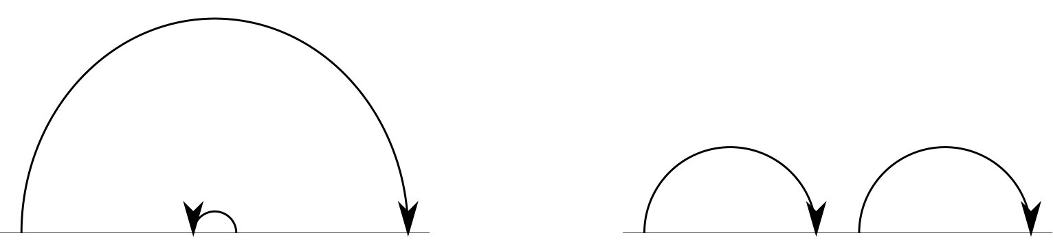 Figure 1
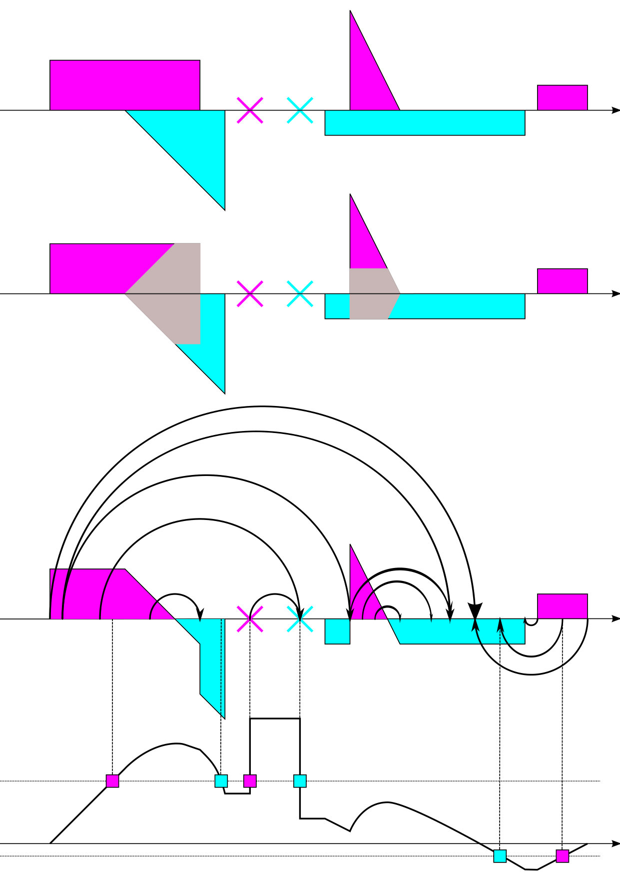 Figure 2
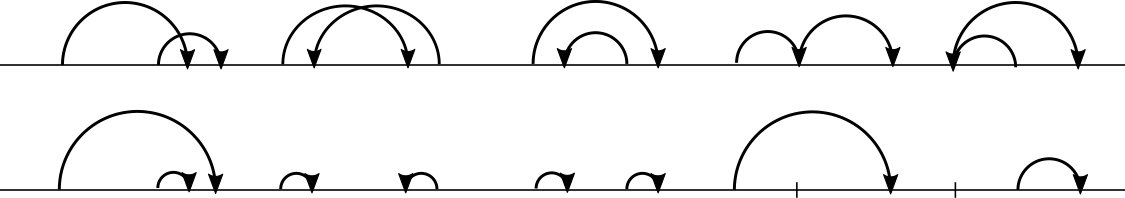 Figure 3
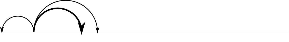 Figure 4
 Figure 5
Peer Reviews
No public reviews on file for this paper yet. If you reviewed it on a platform where reviews are public (OpenReview, ICLR, NeurIPS, ICML), you can paste yours below so the community can read it here.
Videos
No videos yet. Explain this paper in a talk, walkthrough, or lecture? Add one.
On a solution to the Monge transport problem on the real line arising from the strictly concave case
Nicolas Juillet
Abstract
It is well-known that the optimal transport problem on the real line for the classical distance cost may not have a unique solution. In this paper we recover uniqueness by considering the transport problems where the costs are a power smaller than one of the distance, and letting this parameter tend to one. A complete construction of this solution that we call excursion coupling is given. This is reminiscent to the one in the convex case. It is also characterized as the solution of secondary transport problems. Moreover, a combinatoric/geometric characterization of the routes used for this transport plan is provided.
We first introduce the mass transport problem and quickly arrive to our Main Theorem. The reason why it can appear so fast is that it concerns the most basic setting – together with the finite discrete setting – where the optimal transport problem can be introduced, namely the real line for a power cost.
Definition 0.1**.**
Let be a metric space and be a positive real number. We denote by the set of Borel probability measures such that for some (and in fact any) and say that has finite moment of order . The set is the (convex) set of measures with first marginal and second marginal , i.e and where is the -th coordinate function. These definitions naturally extend to positive measures of finite positive mass .
For and two measures with we call “ transport problem” (of Monge and Kantorovich), the problem to minimize
[TABLE]
We denote by the (convex) set of solutions to this problem.
The space is equipped with the weak convergence topology and it is compact according to Prokhorov Theorem, see [Vil03, §1.1.7]. Moreover is continuous on , so that is not empty. One may have a look at page 4.1 where this basic continuity result and a more evolved one are stated and proved. Note that if and have finite moment of order the value of the problem is finite, with . Hence, we will assume that and have finite moment of order permitting a finite value for all the transport problems, for . Note moreover that for every since is continuous and compact, the set is not empty.
Let us review some of the known facts concerning the solutions of the transport problem on the real line . See also Remark 5.7 for the connexion of the transport problem on with the transport problem on geodesic spaces.
- •
For , except from degeneracy occurring when the set of solutions is reduced to a single element, known as commonotonic coupling, quantile coupling, monotone rearrangement, Hoeffding-Fréchet transport or any combination of these vocables. The universality and usefulness of the notion is reflected by this number of names.
- •
The value is the one in the original problem of Monge of 1781 [Mon81] (except that Monge considers or ). For this parameter the quantile transport is still one of the solutions but it may not be the unique one. There is actually a broad class of pairs such that the set of solutions is the whole set of transport plans , see Remark 5.3. Note also that the solutions of the Monge problem in many geodesic space can be disintegrated along transport rays, i.e parts of isometric to intervals where the obtained measures are solution of the Monge problem on the real line. This disintegration is the fundament for many powerful recent applications, see Remark 5.7
- •
The problem for the values may be less known and understood as . However, Gangbo-McCann [GM96] and McCann [McC01] thoroughly explored this range of the parameter . For a class of absolutely continuous measures and , McCann found an algorithm to restrict the search for the solution – it is unique under the absolute continuity assumption – to a finite number of classes, where regions of concerning are mapped onto other regions of concerning , the frontiers between the regions having to be determined. Note that for general values of , the solution space may not be reduced to a single value. Moreover it is not constant as a function of . See Example 2.2 about these two facts. See also Lemma 2.3 the maximal amount of mass that can stay must also stay on place.
- •
Our paper being concerned with the value and its limits , we interrupt here the description of the power costs. It is continued in Remarks 5.1 and 5.2 where we give an account on and, beyond, .
The novelty of this paper is that for the critical and historical parameter we distinguish a special element of that we call the excursion coupling. This element may be seen as a solution for , the counterpart of the quantile coupling that would be the solution for .
Main Theorem**.**
Let and be two probability mesures in , and . The following assumptions are equivalent.
(Solution of the limit transport problem) There exists a sequence with and for every , such that . 2. 2.
(Solution of the secondary transport problem) is in and in this space it minimizes . 3. 3.
(Monotonicity) is concentrated on a set whose arches do not cross, do not connect and have the same orientation when they are nested (see Definition 0.3 and Figure 4). 4. 4.
(Excursion coupling) is the excursion coupling of and as defined in Section 1.
In Section 4 we will prove the Main Theorem as well as the following corollary based on the uniqueness of a coupling satisfying 1 or 2 in the Main Theorem.
Corollary 0.2**.**
Let and be two probability mesures in . The excursion coupling satisfies the two following statements.
- 1’.
For satisfying (with ) and it holds .
- 2’.
For every , the map is minimized by .
The paper is organized as follow: To give the Main Theorem a complete meaning we first briefly make 3. more precise in Definition 0.3 and define in Section 1 the excursion coupling attached to a pair . Note that this definition relies on several facts concerning functions with bounded variations that will be recalled and established in §3.1. Then we prove step by step the following implications: We prove and in Section 2. We prove in Section 3. The fact that there exists at least one solution to the problem and the secondary problem completes the proof (see Section 4). In Section 5 we provide some more comments.
Definition 0.3** (Arches in the Main Theorem).**
Let be a subset , whose elements we call transport routes. In what follows means and the routes are seen as arches (half-circles) over the real line.
- •
The routes of are said non-crossing arches if for every and at least one of the three happens.
- –
- –
for some
- –
One of the two, or , is included in the other.
- •
The arches do not connect means that if , and then .
- •
The nested arches have the same orientation if for every and such that we have .
The first property can be summed up saying that in the plane the two circles of diameter and linking and , and and , respectively, do not cross. The second property states that a point can not be at the same time a starting and arriving point. In the last property is stated that transporting to , and to must be done in the same direction when one of the arches is included in the other. See Figure 4 for a representation of the forbidden configuration and the authorized rerouting – where and are the new routes.
Aknowledgements. I warmly thank Guillaume Carlier, Augusto Gerolin and Martin Huesmann for discussions, bibliographic or editorial suggestions.
1 Definition of the excursion coupling
Given two probability measures and , we consider the signed measure and its cumulative distribution function
[TABLE]
Since it is the difference of and , is càdlàg (right continuous and with left limits at any point) and has limits [math] in . The graph of can be completed at discontinuity points by vertical segments where denotes the left limit at . We denote by the multivalued map defined by at discontinuity points and at continuity points. Its graph is
[TABLE]
and we may also denote it by . If the real is called a generalized solution of .
We further introduce the following subsets of : is the set of increasing points , i.e such that in a neighborhood of any point with satisfies . is the set of decreasing points , i.e such that in a neighborhood of any point with satisfies .
Theorem 1.1** (Excursion couplings can be defined).**
Let and be probability measures and , and be defined as above. One can define a transport of as described in what follows, the results implicitly stated during this construction (see Remark 1.2 for a list) are correct and we call excursion coupling the resulting coupling.
We distinguish two cases (the first one is a special case of the second).
Assume that and are singular measures (). We define a coupling where and . Let be the measure with density . Let be a random variable with law and note where and . Conditionally on and , the random vector is defined to be uniform on . Conditionally on and it is uniform on . 2. 2.
If and with , with probability the random vector satisfies and . On the complementary event, with probability it is distributed as the coupling of the singular measures and defined in the first item.
Remark 1.2*.*
To make Theorem 1.1 a rigorous definition of the excursion coupling we will have to prove that is a probability density, that is almost surely both finite and even with . Moreover, we must prove that the laws of and are and , respectively.
2 Monotonicity of the solutions of the and transport problems
In this section we prove the implications and of the Main Theorem. The name “(cyclical-)monotonicity” in the title is a generic name in Optimal Transport that in this section is represented by property 3. (Cyclical-)monotonicity results are variations of the following simple swapping lemma that concerns the transport problem for cycles of length two. For the transport problem we will firstly interpret Lemma 2.1 for and secondly let go to . For the transport problem will need a result analogue to 2.1 but more specific result: It will be Lemma 2.4 on page 2.4.
Lemma 2.1** (Swapping lemma).**
Let be positive and be in . Assume moreover . Consider a set such that and for any neighborhood of has positive measure (Notice that the support of satisfies these conditions, so that we may choose ). For any and in , the following holds:
[TABLE]
Proof.
Striking for a contradiction, suppose that the opposite identity holds. Then for some there exists such that for every with one has . The two balls (in the -norm) of radius centered in and have positive measure. We choose small enough to make their intersection the empty set. Then it is easily possible to replace by a competitor that coincide with it outside the balls , , and , has marginals and and satisfies (see e.g [GM96, page 129]), a contradiction. ∎
This simple principle, allows for a complete characterization of in the case . We provide it now for the sake of completeness and for further comparison with the limit and secondary problems.
The transport problem for
In this case the identity obtained by applying Lemma 2.1 is equivalent to . This may be graphically represented by the condition that segments in connecting for every the point to are not allowed to cross each other, see Figure 2. These segments may be interpreted as transport routes between concentrated on the line and concentrated on the -axis . The striking fact is that, given and , the elements of being concentrated on such a set are in fact reduced to a single transport plan, called the quantile transport plan. The latter is the law of on the probability space of quantiles, where is the Lebesgue measure and for any a real probability measure , the quantile function is defined as a pseudo-inverse of , namely
[TABLE]
(this infimum is a minimum).
2.1 The transport problem for and the limit transport problem
Important preliminary comparaison to the convex case
In the previous section we recalled that for , provided the transport problem admits a solution with , this trasnport plan is the unique solution and it is the quantile coupling. In particular it is independent of the value of .
The two last assumptions are both false in the case , which we prove in the following example.
Example 2.2*.*
Set and . The set of transport plans is easily described as
[TABLE]
where and . In the case every transport plan gives the same global cost . This proves the non-uniqueness; . Moreover, with the same marginals, depending whether or the measure or , respectively, is the unique optimal transport plan. Hence the solution depends on the value of .
In the two next paragraphs we prove that in the transport problem (for ) arches do not connect and do not cross. In the third next paragraph this will be transmitted to the (limit) transport problem where we also prove that nested arches have the same orientation, completing the proof of in the Main Theorem.
Conclusion concerning coinciding points for
Let satisfying (2) in the swapping lemma, Lemma 2.1 for and be in . Suppose moreover that and coincide meaning that one can take a route from to and a second one from to . Then studying the variations of and considering we see that this can only occur in one of the degenerate case or – compare with the two most right subfigures in Figure 4. With respect to the terminology of Definition 0.3 we have proved that a solution of the transport problem is concentrated on a set whose arches do not connect. This well-known situation has been studied be Gangbo and McCann in [GM96, Proposition 2.9] more than 20 years ago. It yields that can be decomposed as the sum where . Let us remind the argument for the sake of completeness.
Lemma 2.3**.**
If is concentrated on a set whose arches do not connect, it can be decomposed as follows: where and, for denoting the diagonal, it holds . Consequently, is a transport plan with the two marginals singular with respect to each other.
Proof.
Let us write where is concentrated on and is concentrated on . Therefore writes and the marginals of are and . They are respectively concentrated on the two projections and of the set . The fact that these two sets do not intersect is the direct consequence of our assumption. It follows which is equivalent to . ∎
Interpretation of the swapping lemma for and non coinciding points
For the use of the swapping lemma furnishes, compared to , less direct information. Equation (2) may be seen, similarly as in Example 2.2, as a competition of two transport plans, each transporting two points in two other points, in one or the other way. For this reduced transport problem if at most one of the two is true or . Unlike the situation studied for , to determine which transport is better it does not only depend on the relative positions of and with respect to and , respectively, but on the relative positions of the four points. Moreover, even though this ranking of the four point is important and yields the conclusion in configuration and we know since Example 2.2 and Figure 3 that it does not permit to conclude in configuration .
Notation*.*
The notation denotes the configurations of two routes and where or or or , the different alternatives being signed as , , and , respectively.
Since the problem in is in bijection with the one in , when we study configuration we in fact also study . In order to consider all configurations without coinciding points we finally only have to look at , and . Here is the conclusion for these three cases. They are also illustrated on Figure 4 (corresponding, in the same order, to the first three pairs of patterns, from the left).
- •
In the first case is allowed and forbidden. To see that, one can study the variations of where and apply it to .
- •
In the second case is allowed and forbidden. This is a simple consequence of the fact that is increasing.
- •
In the last case, as observed in Example 2.2, it depends on whether or is forbidden or authorized.
With the two first points we have proved that the arches of do not cross.
From the to the transport problem
In this paragraph we prove that the solutions of the transport problem have arches that do not connect, do not cross and have the same orientation when they are nested. This is implication of the Main Theorem.
Consider such that there exists a sequence weakly converging to where for . It also holds , actually an equivalent fact. Hence, if is a closed set and , the equation goes to the limit. In particular this holds for the complementary set of the open set that encodes the condition on non-intersecting arches (first condition of Definition 0.3). As it is satisfied by it is also satisfied by . Therefore is concentrated on a set whose arches do not cross.
Suppose by contradiction that the set of pairs of nested arches that do not have the same orientation has positive measure for . Due to the countable additivity of there exists rational numbers and with such that has positive measure. Since
[TABLE]
for close enough to 1, the open set has measure zero for the corresponding measures . Therefore, it has measure zero for as well, a contradiction. We conclude that concentrated on a set whose nested arches have the same orientation.
The implication finally amounts to prove that is concentrated on a set satisfying the second condition of Definition 0.3: the arches do not connect. Recall from Lemma 2.3 that where has marginals , and . Thus is the limit of the sequence if and only if it can be written where is the limit of . Therefore, has marginals and . Thus there exists and such that is concentrated on . This exactly means that it is concentrated on a set whose arches do not connect.
2.2 The secondary transport problem
Swapping lemma for the secondary transport problem and interpretation
We furnish now a swapping lemma corresponding to the transport problem.
Lemma 2.4** (Swapping lemma for the secondary problem).**
Let be a transport plan such that and for some fixed . There exists a set with such that for any and in it holds
[TABLE]
and if , the following holds:
[TABLE]
Proof.
Let be an optimal transport plan for the primary and the secondary transport problem. Let be . It is the set of routes in the support of such that at some size no mass is transported from the ball of center and radius to the left of at distance less than . We have . The proof of this result is postponed to Lemma 2.5. The symetricaly defined sets , and have measure zero too (for instance here denotes the set ). We define now as where is any set, as for instance , satisfying the condition in Lemma 2.1. Observe that .
We are now ready for the proof. It is almost identical to that of Lemma 2.1 that we invite the reader to read again: the principle is that is compared to a competitor defined rerouting part of the mass around and to mass aroud and . From Lemma 2.1 we note that (3) is satisfied for any . Aiming for a contradiction, suppose that for some routes and in it holds at the same time and . Until the end of the paragraph let us see that without loss of generality we can assume : The first equation induces ‘ or ’. Without loss of generality we can assume the first case. The second inequality implies and and without loss of generality we assume . This finally implies .
Apparently the swapping method used in the proof of Lemma 2.1 that consists in picking mass in equal quantity around the points , , and can be applied without problem providing a competitor with , a contradiction. However, this argument only works if and not directly if because can not be certified: during the swap the routes and with have a priori in their neighborhood routes and with that do no longer satisfy (3), so that is made possible. The relation is no longer a contradiction because . In this critical situation let us call the point . As and are not in we can swap selecting the mass on the proper side of . More precisely for there is some mass traveling from a neighborhood (as small as we want) of to a small right neighborhood of . There is the same mass on a small left neighborhood of transported to a small neighborhood of . We swap for defining : the mass around is transported around and the mass directly on the left of is transported directly to the right of . We obtain and keep .
∎
Lemma 2.5**.**
Let be a solution to the secondary optimal transport and be . Then .
Proof.
Fix two rational numbers. Consider the set of points such that there exists with and moreover . Then every point is in the support of the measure defined by , but it is also isolated on the left in the sense that for small enough. One can easily convince that there are countably many such points and they are not atoms. Therefore, and . Finally, since we find . ∎
We can now give the geometric meaning for the routes of set as in Lemma 2.4. As for the problem we compare the different configurations with their alternative – recall the list on page 2.1 – and again these comparaisons are illustrated on the three most left patterns of Figure 4.
- •
Pattern is allowed and forbidden. To see that, since we have to look at the secondary problem.
- •
Pattern is allowed and forbidden because as in the problem, (3) is a strict inequality.
- •
Finally, pattern is allowed and is forbidden because as in the problem, (3) is a strict inequality.
Some of the points may be equal. Swapping does not change the cost if or . We have only to look at and and see that it is never better than and (see on Figure 4 the two patterns on the right).
- •
For the pattern , meaning , we have but the secondary problem tells us to choose in place of .
- •
For , from the primary problem we choose in place of .
Finally as for the limit transport problem, we have proved that if is a solution of the secondary transport problem it is concentrated on a set whose arches do not cross, do not connected, and have the same orientation when they are nested.
3 Transport plans concentrated on monotone sets of arches are the excursion coupling
3.1 Proof of Theorem 1.1 defining the excursion coupling
We need to explain why Theorem 1.1 can define the excursion coupling. We only need to investigate the construction in case 1 where and are singular (), which we thus assume in the present subsection.
With the following lemma we will be able to handle with as if it were a continuous function.
Lemma 3.1** (Generalized intermediate value theorem).**
For any càdlàg function , any and such that and , there exists such that .
Proof.
Let , be as in the statement. Without loss of generality we assume , and . Let be the infimum of . As it is a not empty set. As moreover is right continuous we have and . Due to the definitions of and , any satisfies . If is left-continuous at we have . If it is not, as we also have . ∎
A result by Bertoin and Yor establishes a relation between the occupation measure in a set of a function of finite variation and its variations when its values are in , see Remark 5.5 for details. In particular we can apply their Theorem 1 in [BY14] (see also their §5) to and , and relate the total variation (without its saltus part) with the number of solutions of the equations , where goes over : For any points in
[TABLE]
where
[TABLE]
is the so-called Banach indicatrix, after [Ban25]. Notice that in [BY14] the result is stated for and . Our statement on a general interval is a trivial generalization. Another difference is that we only apply the formula for the occupation measure of in when . It is hardly more than a simple exercise to rewrite (5) for generalized solutions of , which permits at the same time to forget about the saltus part. For this purpose we introduce the generalized Banach indicatrix. Let be in .
[TABLE]
Therefore (5) yields
[TABLE]
A consequence of Theorem 1 in [BY14] specifies that not all intersections with the graph need to be considered. Recall first that and have been defined in Section 1. Bertoin and Yor proved that almost surely for , the (generalized) Banach indicatrix equals where
[TABLE]
(with obvious notation Bertoin and Yor in fact proved the equality for the non yet generalized indicatrix .) This also comes from Theorem 1 in [BY14] (where ):
[TABLE]
With the next result we go further in the analysis.
Proposition 3.2**.**
For almost every , the set has cardinal a finite and even integer. In fact for almost every it holds with . Moreover if the generalized solutions of are alternatively crossing positively and negatively, starting with the most-left solution if and if .
Proof.
Due to (6) the generalized Banach indicatrix is finite for almost every and with (7) for almost every we have . With the generalized intermediate value theorem (Lemma 3.1) and as we conclude that is an even number for almost every .
More precisely, due to the generalized intermediate value theorem applied to and reminding that this function has limit zero in and the points of are ordered with and if , and if . ∎
Coming back to (6), another direct generalization of Bertoin and Yor’s study is
[TABLE]
It will be useful for recovering and from .
For any measurable set , let denote the following positive measure
[TABLE]
We consider in particular and and and call , and the corresponding measures. As a consequence of Proposition 3.2 and of the concerned definitions we can already state and . The next result indicates the other projections.
Proposition 3.3**.**
The measures and defined as in the previous paragraph satisfy and .
Proof.
From (6) and (8), computing the half sum and the half difference we already have
[TABLE]
Therefore,
[TABLE]
and . Recall moreover the definitions
[TABLE]
where and are the positive and negative parts of . As , there exists with and . By outer regularity for every there exists an open set such that and .
Finally from the -additivity of measures and the fact for every there exists a finite union of semi open intervals such that and . The partition of given by permits us to check that the positive total variation of is greater than which is greater than . This holds for every so that . Symmetrically . Finally as we conclude with and . The same identity is correct on with the same proof (for instance ). ∎
Proof of Theorem 1.1.
We proved that is almost surely an even integer and . Due to Proposition 3.2 is concentrated on and is distributed as . Similarly is concentrated on and distributed as . Finally the law of is and the law of is . ∎
3.2 Proof that a transport plan concentrated on a monotone set is the excursion coupling
In this subsection we call monotone a set with arches that do not cross, do not connect and have same orientation when they are nested. In what follows we prove of the Main Theorem, i.e. that measures concentrated on a monotone set are the excursion coupling of their marginals (this is correct even though these measures do not have finite first moment). We prove this first in the case and prove the general case on page 3.2.
Proof of for measures
The generalized , and the related objects are still defined as above and we still assume . We define (that depends on ) as
[TABLE]
where is the set of levels such that and are the points of . We stated in Proposition 3.2 that has full measure with respect to . Therefore, with respect to the definition of the excursion coupling, we have .
Remark 3.4*.*
We could prove that is monotone (the arches of do not cross, do not connect and have the same orientation when they are nested). Since , this would correspond to the implication . This is correct and can be proved directly but our proof of the Main Theorem goes .
Proposition 3.5**.**
Let and be mutually singular measures of and be a monotone transport plan in . Let be a monotone set with . Then is still monotone and satisfies .
Proof.
It is not a priori known that and this statement is in fact clearly equivalent to the proposition result. Let be as in the statement. We will define such that has measure zero for and . Hence we will have .
Let and be as in the statement. Let be the diagonal and and . Let be and . Finally .
Proof of . We already recalled in Lemma 2.3 that transport plans , whose arches do not connect takes the form where . As we have and . We have . Similarly, so that . Finally there are countably many pairs with and . Thus and =1.
Proof of . Let be in . Without loss of generality we can assume ( became impossible as was replaced by ). Let us first prove
[TABLE]
If not there exists with and (or the same property inverting the role of and ). As is dense in the same is correct for a point , which leads to a contradiction with the monotonicity of , whose arches should not cross.
Case 1: Assume ; the complementary case is considered further in case 2. Then . Moreover, a similar argument as for (15) shows that for any we have
[TABLE]
In fact would imply that there exists some with and . If this contradicts the fact that arches and do not cross. If the latter fact or the one that nested arches have the same orientation is violated. From (16) we find for every . As and ( is not possible because is in so that it can not be an abscise of the decreasing part of ) the multivalued function is single valued at . Hence, from the definition of involved in it follows that must be an element of . Therefore, since the level cuts in points of or it is not possible to have for (In a neighborhood of we would have ). It follows that and are consecutive zeros of . Thus .
Case 2: We want to finalize the inclusion looking at the pairs where or is an atom of . Since the arches of do not cross at least one of the two is true: i) has empty intersection with ), or ii) has empty intersection with (recall that here ), i.e the arches of the left and right patterns of Figure 5 can not all be in . Without loss of generality we will assume that is empty. This corresponds to the two first patterns from on Figure 5. Adapting the argument of case 1 we find and in place of . Thus is in . Let be in . We have . This is due to the fact that the arches starting from have the same orientation as and do not cross it. Moreover, for some additional mass in could arrive from . We want to prove that is also true for any . If is not an atom we can proceed as before starting with and the arche with . Therefore we assume that is an atom of . If we will be able to conclude easily that there exists and we conclude as we did twice before (on the generalized function can not only touch the level but it must cut it, which is not possible because for the level ). In the other case and all the mass arriving in comes from . Therefore may be an element of but not of , a contradiction. This case can not happen and we proved in all the other cases. Finally we proved .
∎
Proposition 3.6**.**
Let and be singular measures and the excursion coupling and as defined in (14). Let be another coupling concentrated on . Then .
Proof.
Let be the set of atomic points of and the set of atomic points of . From the definition of we see that the set is contained in the graph of a function from to . The same is true, inverting the coordinates for . Hence the measures and coincide on the set that we denote by , i.e
[TABLE]
Therefore we aim at proving that and coincide on the countable set . We will in fact prove for every . Let be in . Let us assume without loss of generality . We further assume so that according to the definition of the transport plans and are concentrated on it and the mass of on must be transported onto . This writes and we have also . Reasoning similarly we obtain . Therefore
[TABLE]
The construction of associates the route with to some level . The generalized intermediate value theorem, Lemma 3.1 permits us to derive for every so that it also holds . Therefore (17) can be written for any such that in place of . Recall that it also holds for in place of . We will be done if we can prove . This is in fact correct because
[TABLE]
∎
Proof of for general measures in
We no longer assume . In this case we know from Lemma 2.3 that any satisfying 3 in the Main Theorem can be written in the form where satisfies . We are in the situation of the last paragraph because and satisfies 3: since we know that there is a monotone set with it also holds . From the discussion above we obtain that is the excursion coupling of and . This exactly implies that is the excursion coupling of and .
4 Final elements of proof of the Main Theorem and its corollary
Proof of the Main Theorem.
The structure of the proof is the following:
- •
The set of measures satisfying 1 (the solutions to the problem) is not empty.
- •
The set of measures satisfying 2 (the solutions to the problem) is not empty.
- •
Assumption 1 implies 3 and assumption 2 implies 3 (see Section 2).
- •
Assumption 3 implies 4 (see Section 3).
- •
There is a unique and well-defined coupling satisfying 4 (see Theorem 1.1).
Therefore, if satisfies 4 it equals any coupling satisfying 1, respectively 2. As these sets are not empty, if satisfies 4 it also satisfies 1, respectively 2.
We proved everything except the two first existence statements. They will be obtained as consequences of Lemma 4.1 that is proved in this section. ∎
Il order to prove that there exists a solution to the limit transport problem (property 1) it suffices to remind of two elementary facts. First, any sequence in admits cluster points. The set is indeed a compact set for the weak topology, as a simple consequence of Prokhorov Theorem and of the fact that it is closed. Second, as we recalled in the introduction, the set is not empty for every . These two elements permit us to conclude that there exists at least one element that satisfies 1. However, the non emptiness of relied on the following Lemma 4.1 through the standard argument of optimization. We prove it now for the sake of completeness and in order to prepare the proof of Lemma 4.3.
Lemma 4.1**.**
Let and be as in the statement. Let be in and be two mesures with finite moment of order . The function
[TABLE]
is continuous on , endowed with the weak topology of laws on .
Proof.
For every we decompose as the sum of a bounded continuous function and a reminder function:
[TABLE]
where denotes the positive part of . Since we have
[TABLE]
so that for every . Thus . Let us finish proving that is continuous at . Let be a positive real number and large enough to make smaller that . Now
[TABLE]
As is continuous and bounded this estimate proves that there exists a neighborhood of such that for every it holds . ∎
Remark 4.2*.*
Until now, even though it is clear from the context and a consequence of the Main Theorem (implication ) we never proved that a so-called solution to the limit transport problem is a solution to the transport problem. The next result may be invoked to prove it directly.
Lemma 4.3**.**
The function is continuous.
Proof.
Let us fix . For another pair we have
[TABLE]
Let . Due to the dominated convergence theorem the term is smaller than for in a neighborhood of . For large enough is smaller that . For this fixed we see that the last term is smaller than when is in a certain neighborhood of .∎
Let us now prove that the set of solutions to the secondary transport problem is not empty. With what precedes including Lemma 4.1 we indeed know that is not empty and that it is closed. Let be a minimizing sequence for on . This is a continuous function so that is not empty.
We finish the section with the proof that seemingly stronger results are equivalent to 1 and 2 in the Main Theorem.
Proof of Corollary 0.2.
The Main Theorem applies to any subsequence that is increasing. Therefore, in the compact set any subsequence of possesses an increasing subsequence converging to . This proves 1’.
Let be an exponent smaller than . Then the Main Theorem applies for . ∎
5 Concluding bibliographic remarks and perspectives
Remark 5.1* (the transport problem).*
For the cost function is where is the distance on . This corresponds to the coupling problem that defines the total variation of and . A coupling is a solution if and only if it writes and .
Remark 5.2* (the transport problem for ).*
For the cost function where is the distance on is singular on the diagonal where it takes the value . Notice that it writes where is decreasing, convex and has limits and [math]. This type of cost, including the Coulomb cost has been thoroughly studied by Cotar, Friesecke and Klüppelberg in [CFK13] with the purpose of determining the joint distribution of electronic particles on their orbitals. Their Theorem 3.1 states an existence and uniqueness result for measures admitting a density. In §4.1 they conduct a precise study of the one dimensional case in the spirit of [GM96, McC01], the same geometric spirit that is also inspiring us in the present paper. Concerning the Coulomb type costs, notice that the assumption is the natural one for the chemical application. In their Theorem 4.8 the authors completely characterize the optimal transport for an absolutely continuous measures with positive density. As for this solution does not depend on the particular value of (or of ).
However, there is no uniqueness of the optimal transport plan in general, as can be seen for instance with the example . Moreover the example , with is similar to Example 2.2: For the problem admits a unique solution , for another transport plan is the unique solution and for the solutions are the plans defined by .
Remark 5.3* (On the solution of the Monge problem selected in [DML18]).*
It is clear that if there exists such that and are concentrated in and respectively, then coincide with the set of all transport plans between and . In fact for measures with finite first moment if and only if there exist such a real splitting the supports of and (but the symmetric situation is possible). For general measures the set has recently be described by Di Marino and Louet in [DML18]. This recent paper concerns another way to select a special element of when the entropy parameter in the entropic regularized Monge problem tends to zero. Note that the resulting coupling is different from ours. If the measure are as in the beginning of this remark, the plan of Di Marino and Louet is . We obtain the decreasing rearrangement, i.e the law of seen as a random vector on .
Remark 5.4* (On the Skorkhod problem for unbiased Brownian motions).*
One motivation to our paper was to better understand a work by Last, Mörters and Thorisson [LMT14] and reformulate their construction in the framework of the optimal transport theory. In this paper eternal Brownian motions starting in are embedded onto with non-negative random time such that is an eternal Brownian motion independent of . The authors define a coupling similar to our excursion coupling but for two -finite random measures on . This solution minimizes for any concave function . Comparing with our case that concerns deterministic measure one can conjecture that among couplings with law in that satisfy the constraint , the excursion coupling is the one minimizing for every .
Remark 5.5*.*
Bertoin and Yor [BY14] established their deterministic formulae in relation with an important chapter of Stochastic Calculus. The occupation measure of (the continuous part of) a real semimartingale turns out to be a random absolutely countinuous measure with density expressed in terms of local times, that are quantities described by the Meyer–Tanaka formula. The work of Bertoin and Yor provides analogue results in the deterministic word of functions with finite variation.
Remark 5.6* (Sharpness of the assumptions).*
The assumptions in the Main Theorem are by no mean claimed to be sharp. For property 1, a rough analysis of the proof seems to indicate that the family of costs defined by can be replaced by any family of type where it is assumed for every and is increasing and strictly concave. Concerning property 2, any of the same type as before should play the same role as . Finally, the fact that and have a finite first moment should not be necessary to state the equivalence between 3 and 4 (see also Remark 3.4).
Remark 5.7* ( limit transport problem in Euclidean spaces).*
The transport problem for the Monge distance cost in Euclidean and further in some more general geodesic spaces is a research stream with a rich history. It recently culminated with the optimal transport proof by Cavalletti and Mondino of the Lévy-Gromov inequality [CM17]. It is intimately connected to the Monge problem on the real line because under appropriate assumptions on the space and the marginal measures, any optimal transport plan can be disintegrated as a mixture of one dimensional transport plans concentrated on disjoint geodesic rays.
A natural question with respect to the present paper is the existence and uniqueness of a solution to the limit problem in Euclidean spaces. One can moreover conjecture that such a cluster solution can be disintegrated in a way that the transport along the geodesic rays always is the excursion coupling. A similar result has been proved in [AP03] for the limit problem and the quantile coupling.
Remark 5.8* (Generating by picking a random point on a tree).*
A popular construction in probability is to associate a random tree with a random function (or process) . Typically in the construction of the continuum random Brownian tree [Ald93] a random tree is associated to a random excursion. However this topological construction is purely deterministic. Let be function defined on an interval . We write if and only if and . The tree is the quotient space . The fact that we conducted a similar operation with our function yields an appealing interpretation. In place of choosing a random point on the -axis with density and continue selecting uniformly an excursion among possible we could directly choose randomly a point on the associated tree according to the length measure, i.e the Hausdorff measure of dimension . Doing this we come closer to the classical simulation of the quantile coupling where a point is chosen on the tree (a segment) according to the length measure (the Lebesgue measure). While it is clear that the measure on the tree is the correct one if and are simple, e.g finite sums of atoms, or such that is of class with finitely many changes of monotonicity, it is not is the general case. We leave it as a conjecture that the quotient measure on the tree corresponding to our generalized function always is the length measure.
The reference list from the paper itself. Each links out to its DOI / PubMed record.
- 1[Ald 93] D. Aldous. The continuum random tree. III. Ann. Probab. , 21(1):248–289, 1993.
- 2[AP 03] L. Ambrosio and A. Pratelli. Existence and stability results in the L 1 superscript 𝐿 1 L^{1} theory of optimal transportation. In Optimal transportation and applications (Martina Franca, 2001) , volume 1813 of Lecture Notes in Math. , pages 123–160. Springer, Berlin, 2003.
- 3[Ban 25] S. Banach. Sur les lignes rectifiables et les surfaces dont l’aire est finie. Fundam. Math. , 7:225–236, 1925.
- 4[BY 14] J. Bertoin and M. Yor. Local times for functions with finite variation: two versions of Stieltjes change-of-variables formula. Bull. Lond. Math. Soc. , 46(3):553–560, 2014.
- 5[CFK 13] C. Cotar, G. Friesecke, and C. Klüppelberg. Density functional theory and optimal transportation with Coulomb cost. Communications on Pure and Applied Mathematics , 66(4):548–599, 2013.
- 6[CM 17] F. Cavalletti and A. Mondino. Sharp and rigid isoperimetric inequalities in metric-measure spaces with lower Ricci curvature bounds. Invent. Math. , 208(3):803–849, 2017.
- 7[DML 18] S. Di Marino and J. Louet. The entropic regularization of the Monge problem on the real line. SIAM J. Math. Anal. , 50(4):3451–3477, 2018.
- 8[GM 96] W. Gangbo and R. J. Mc Cann. The geometry of optimal transportation. Acta Math. , 177(2):113–161, 1996.