Short-term prediction of Electricity Outages Caused by Convective Storms
Roope Tervo, Joonas Karjalainen, Alexander Jung

TL;DR
This paper introduces a machine learning framework for predicting power outages caused by convective storms by tracking storm cells using radar images and classifying their damage potential, addressing data imbalance issues.
Contribution
A novel approach combining radar image analysis and machine learning to predict storm-induced outages, with a focus on storm cell tracking and damage classification.
Findings
Random forest and deep neural networks evaluated for classification.
Storm cell tracking improves outage prediction accuracy.
Handling imbalanced data remains a key challenge.
Abstract
Prediction of power outages caused by convective storms which are highly localised in space and time is of crucial importance to power grid operators. We propose a new machine learning approach to predict the damage caused by storms. This approach hinges identifying and tracking of storm cells using weather radar images on the application of machine learning techniques. Overall prediction process consists of identifying storm cells from CAPPI weather radar images by contouring them with a solid 35 dBZ threshold, predicting a track of storm cells and classifying them based on their damage potential to power grid operators. Tracked storm cells are then classified by combining data obtained from weather radar, ground weather observations and lightning detectors. We compare random forest classifiers and deep neural networks as alternative methods to classify storm cells. The main challenge…
Click any figure to enlarge with its caption.
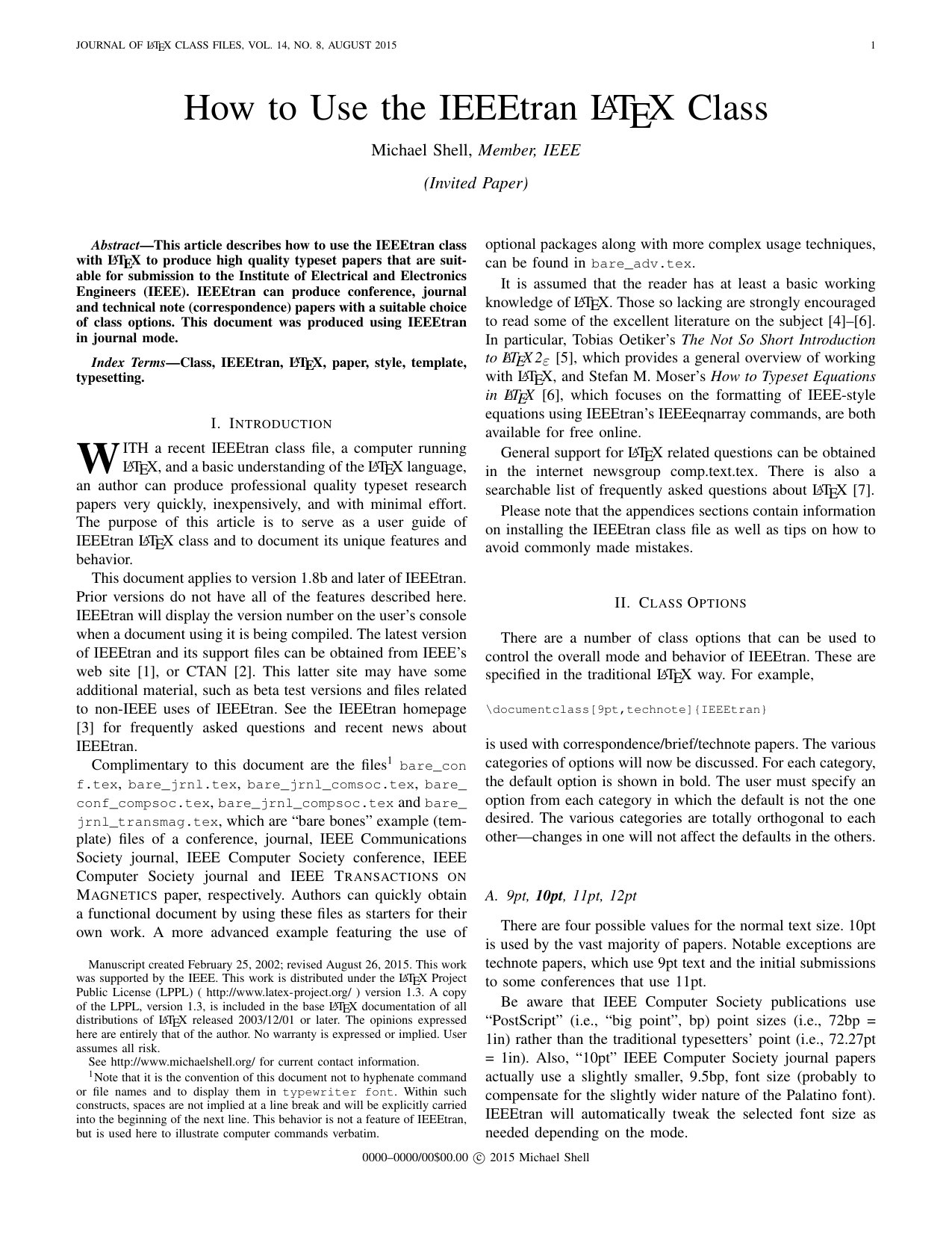 Figure 1
 Figure 2
 Figure 3
 Figure 4
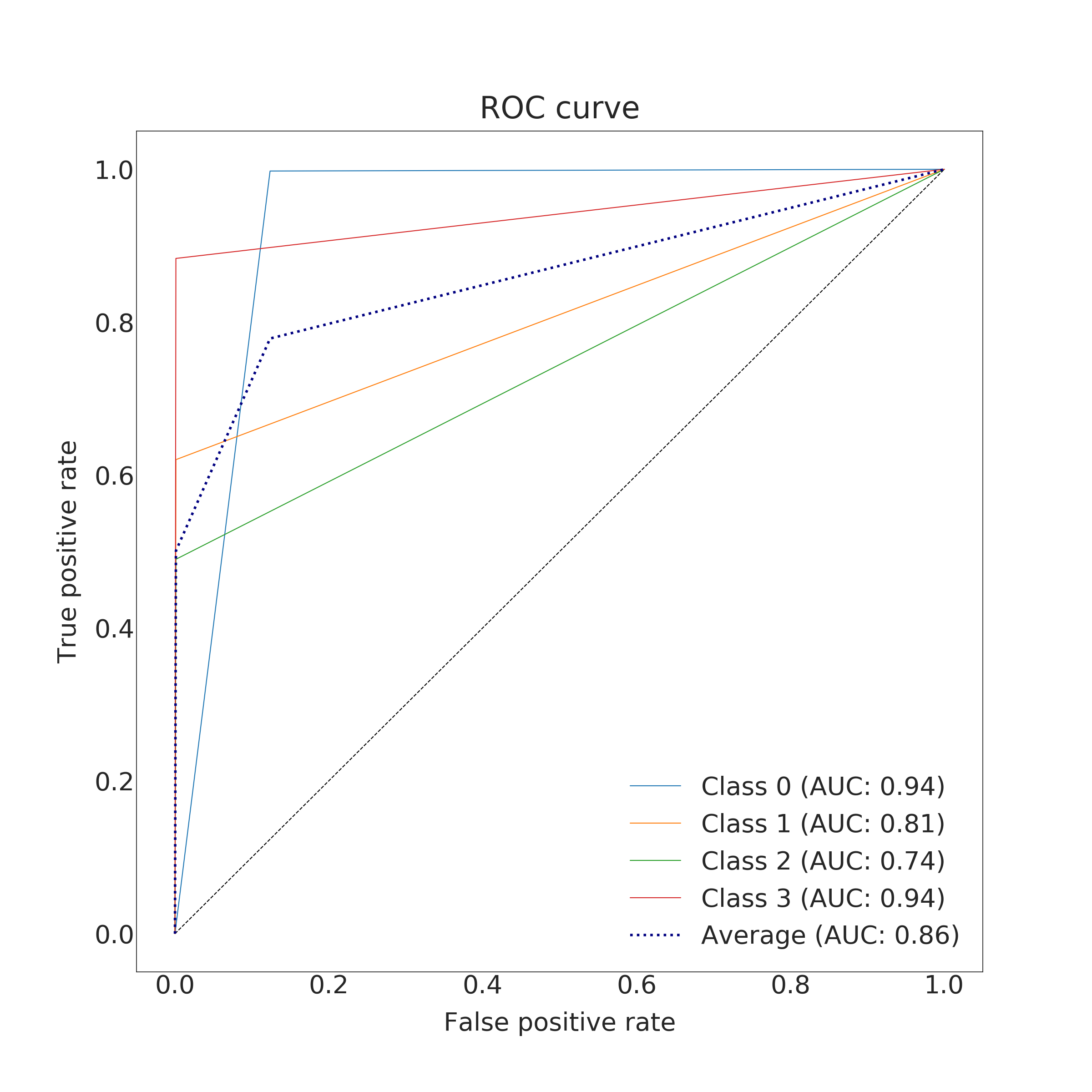 Figure 5
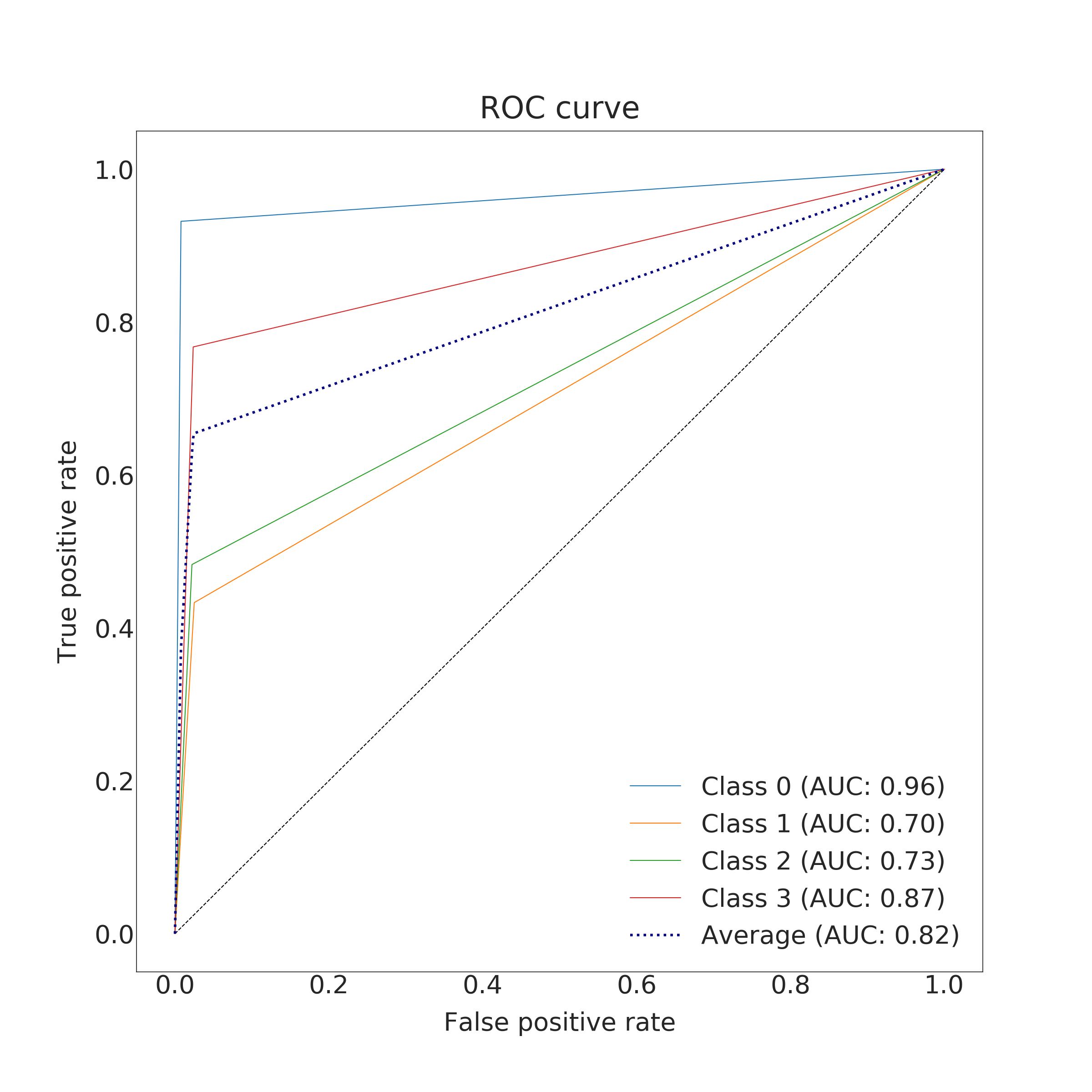 Figure 6
 Figure 7
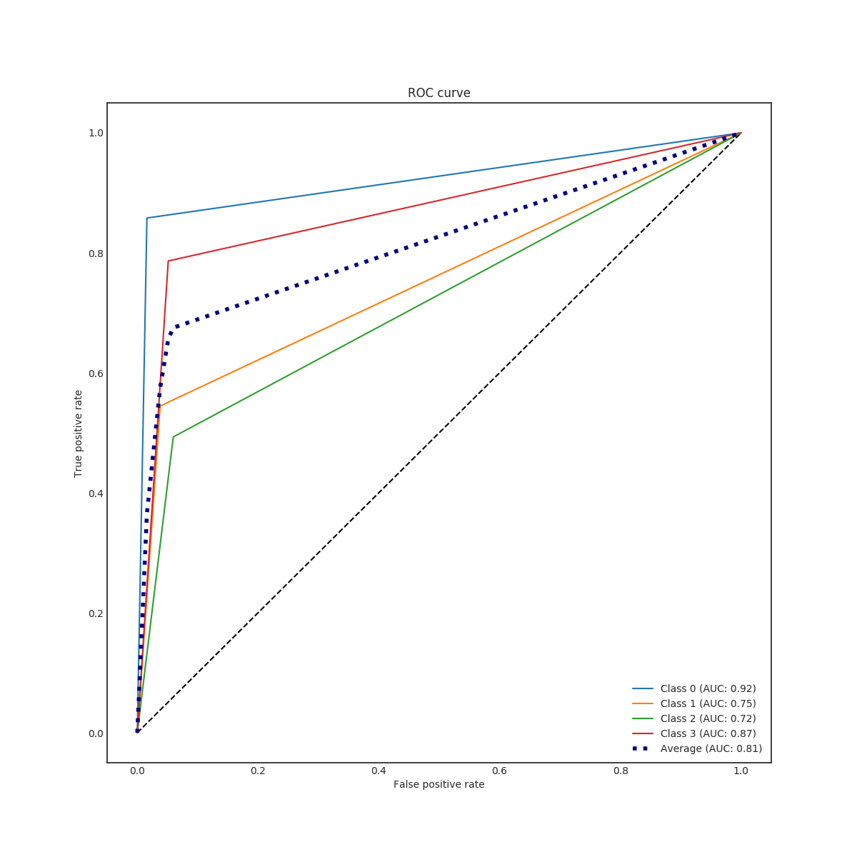 Figure 8
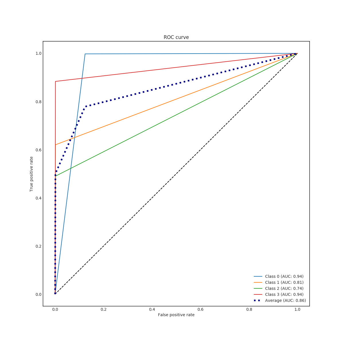 Figure 9
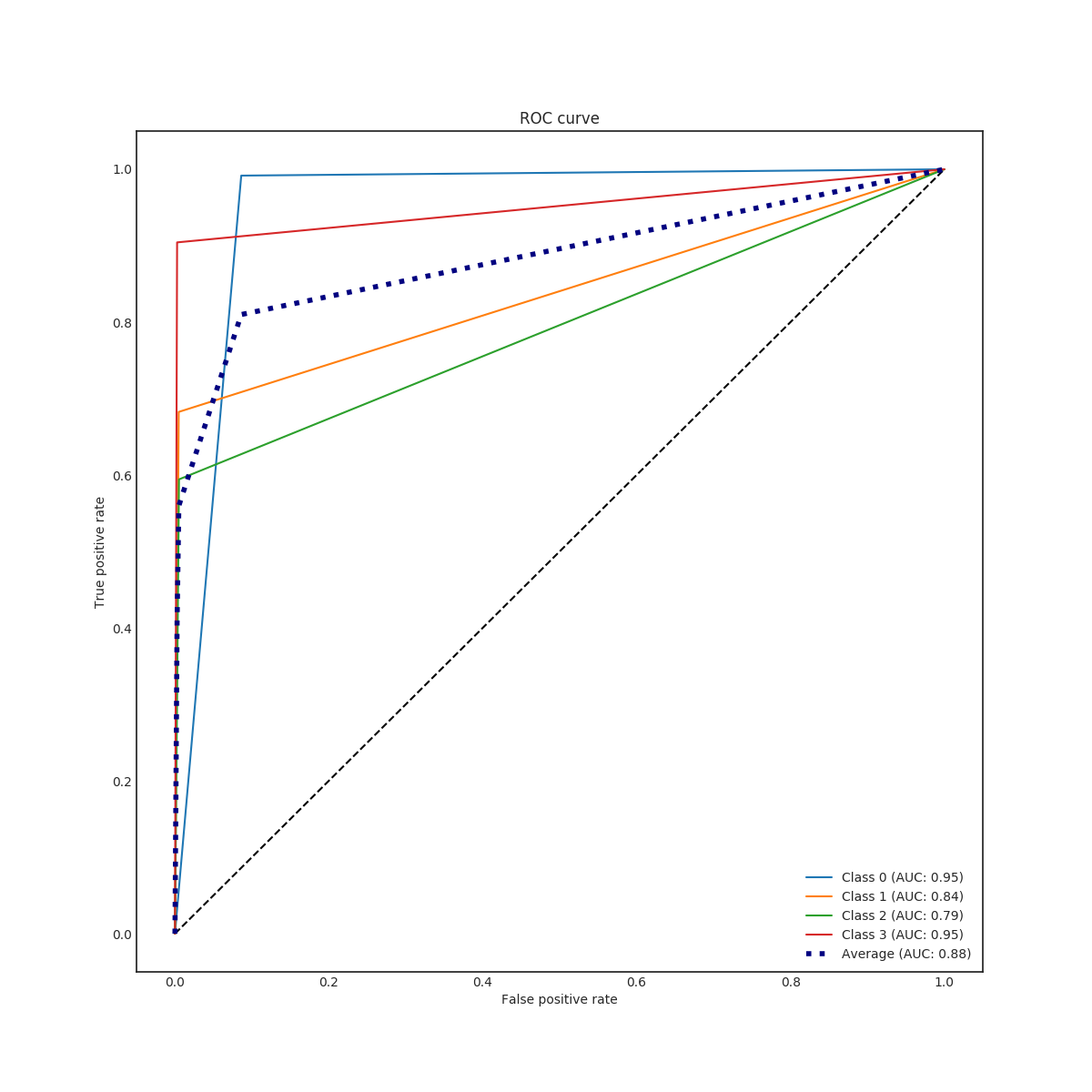 Figure 10
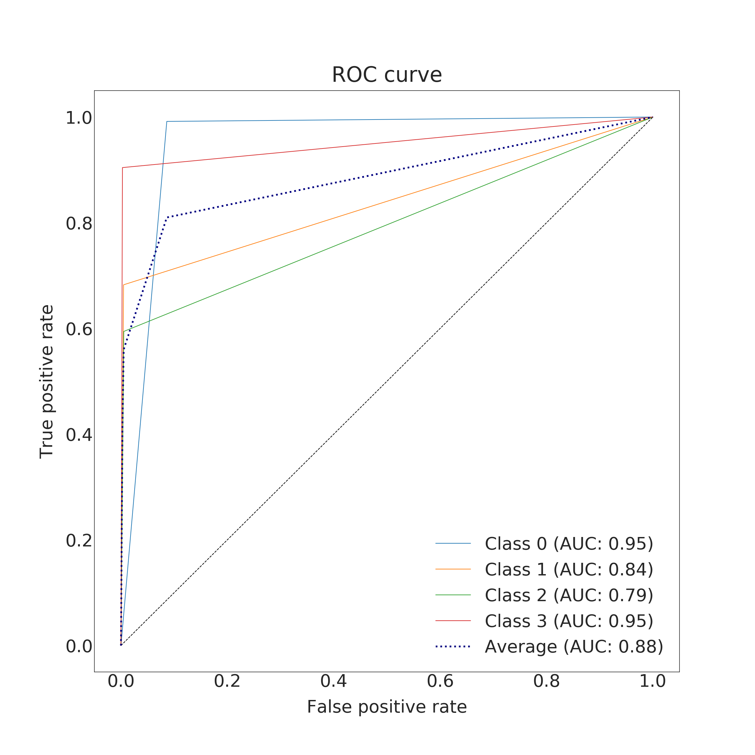 Figure 11
 Figure 12
 Figure 13
 Figure 14
 Figure 15
 Figure 16
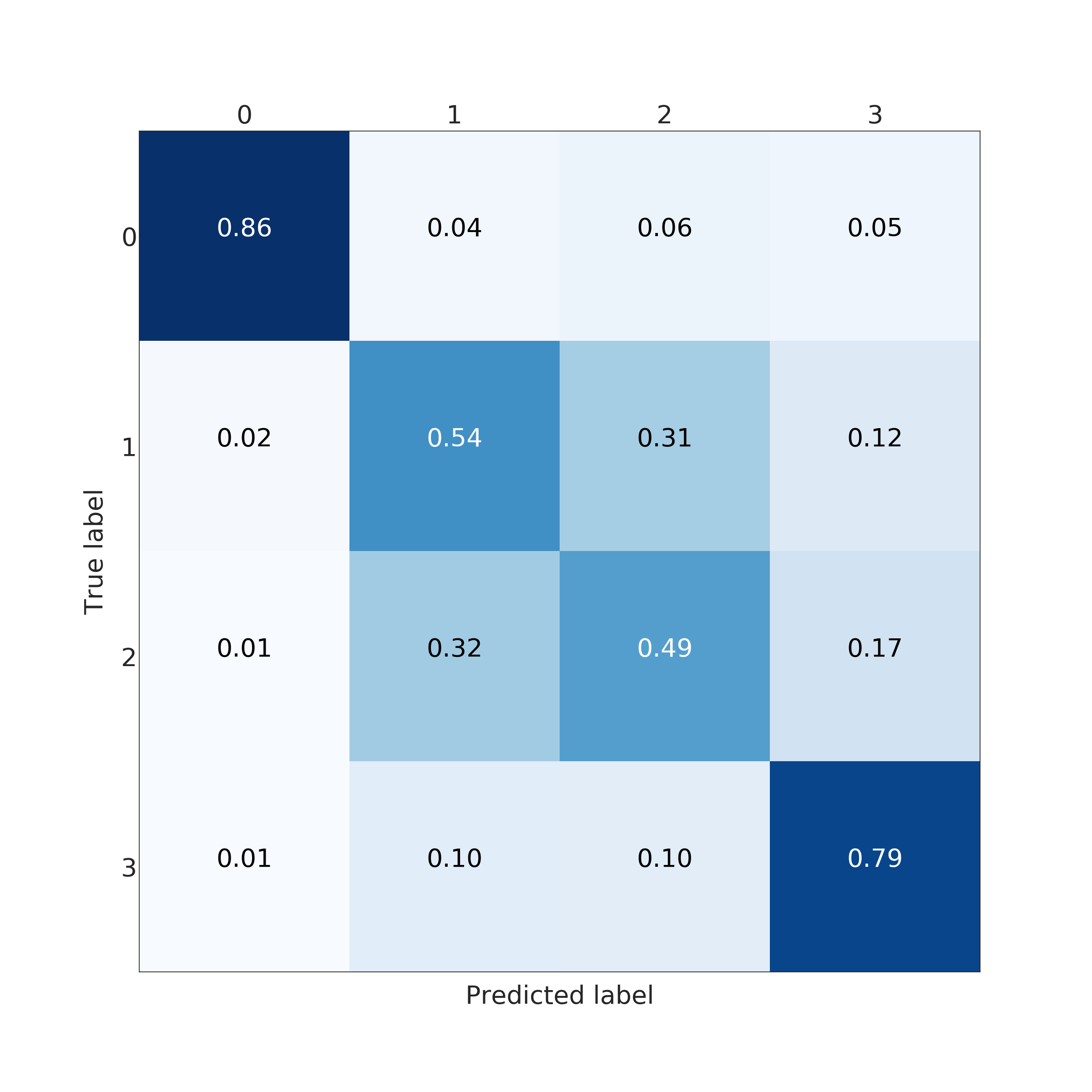 Figure 17
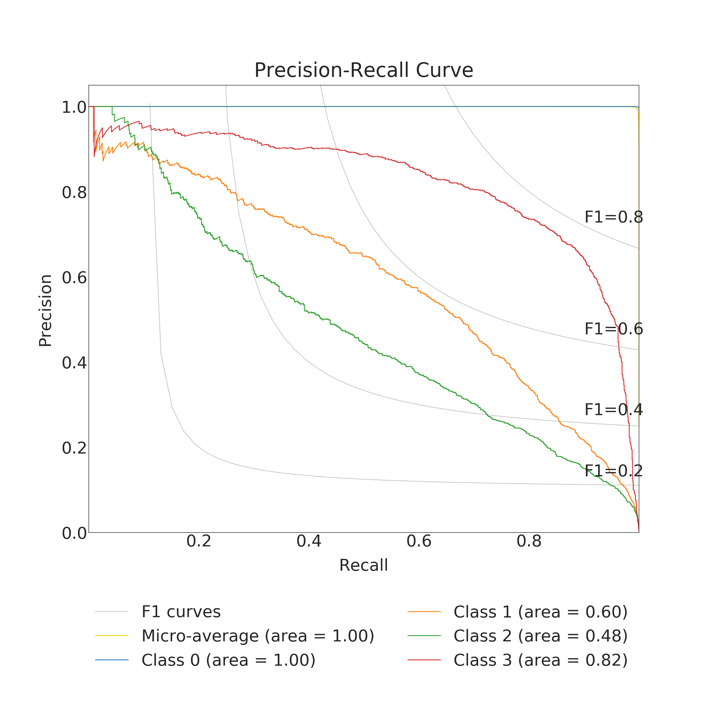 Figure 18
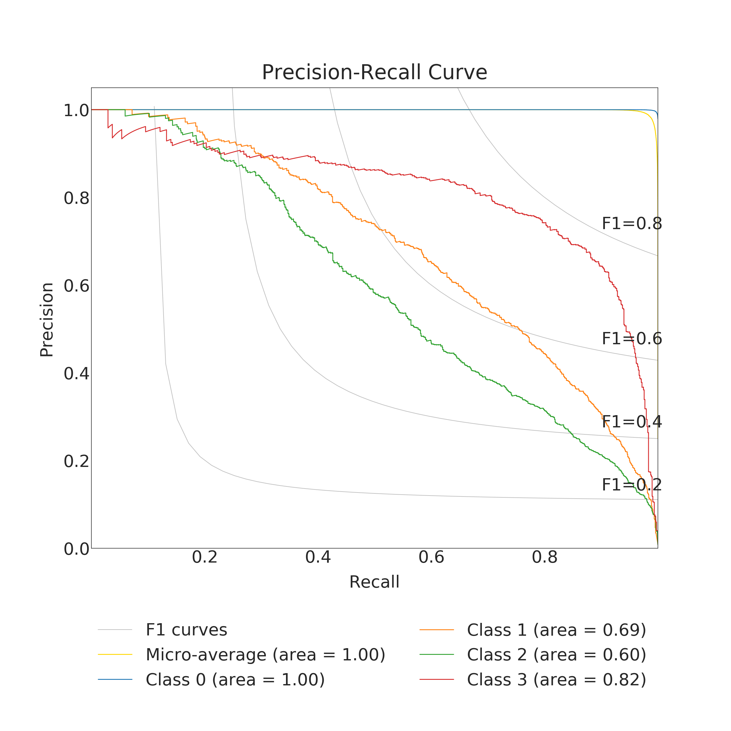 Figure 19
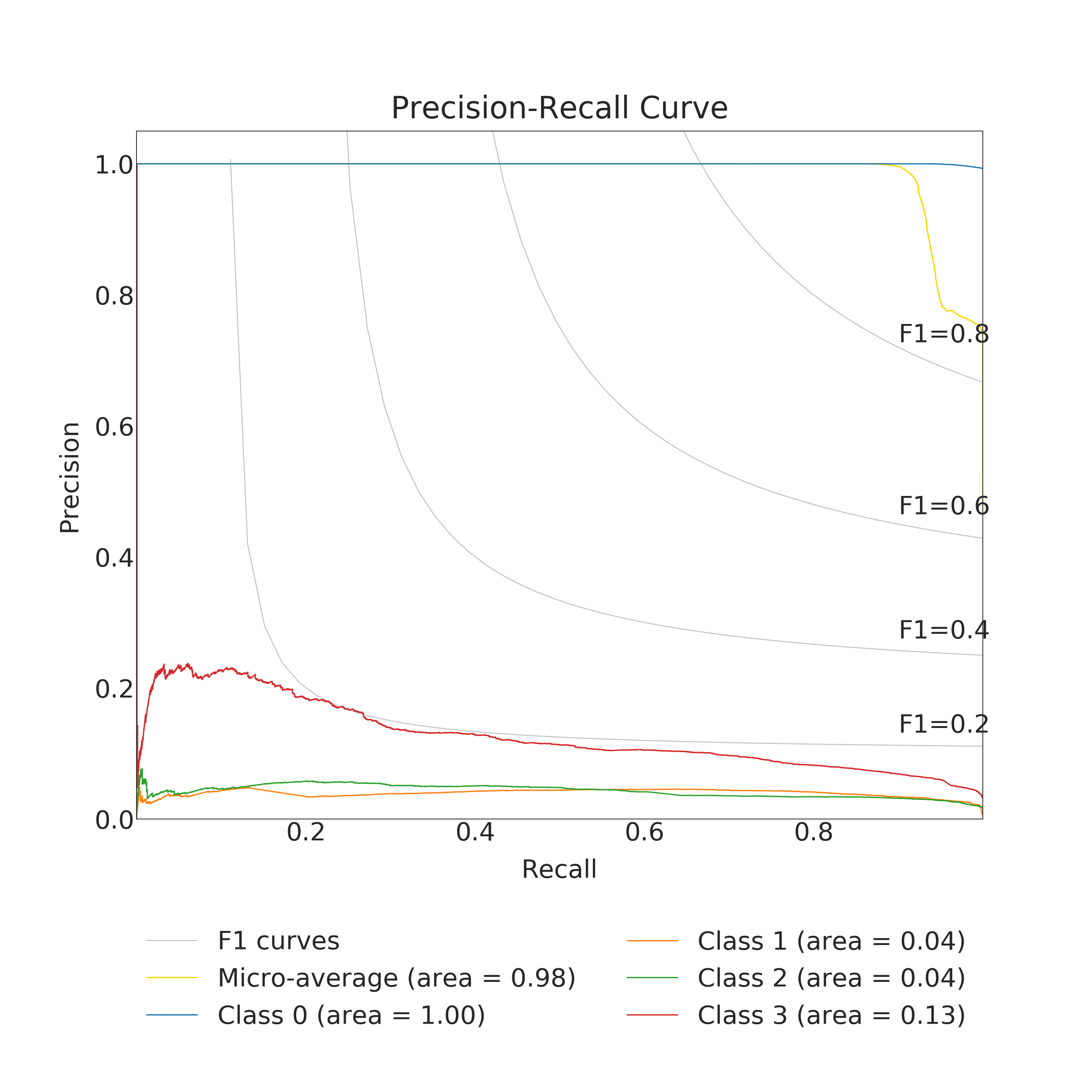 Figure 20
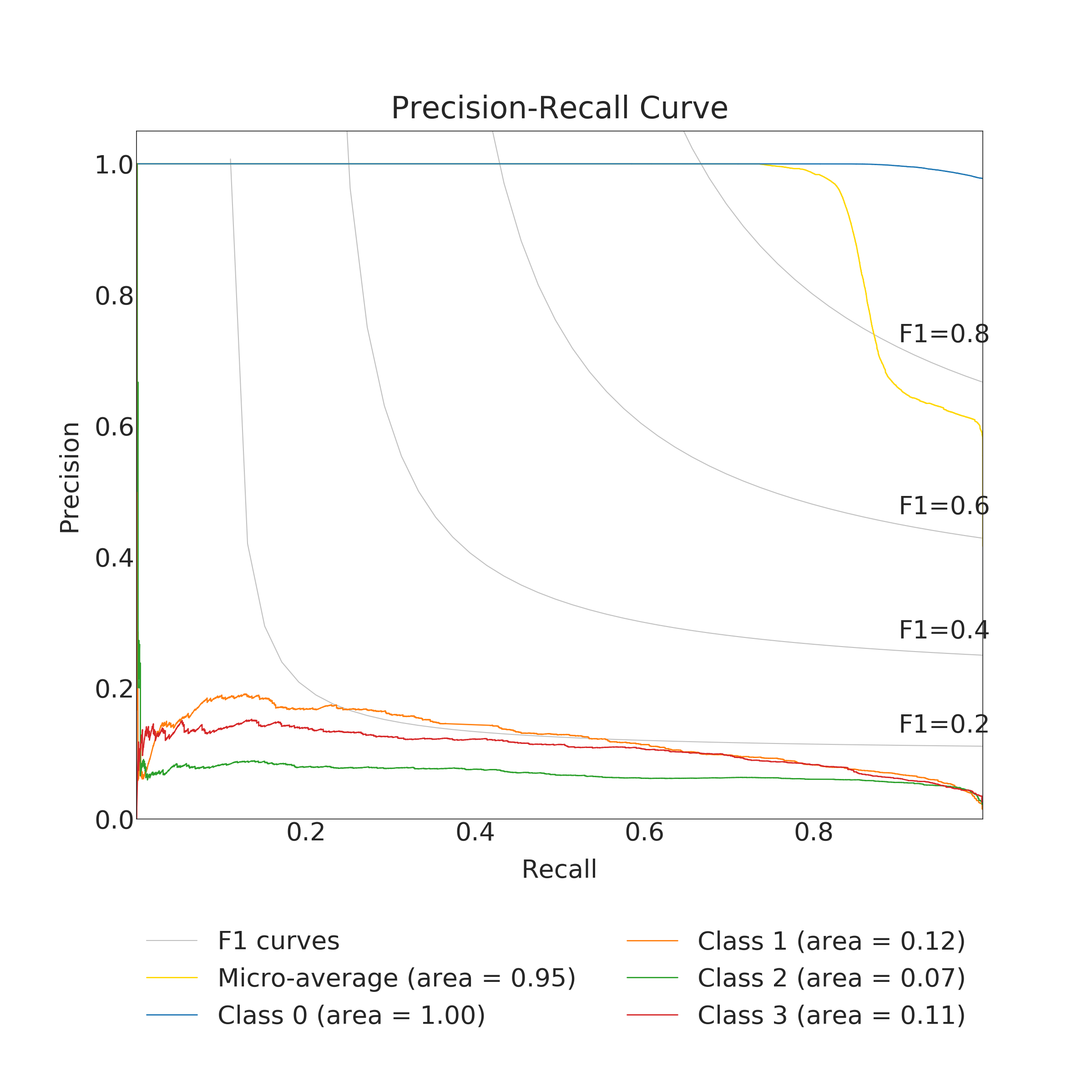 Figure 21
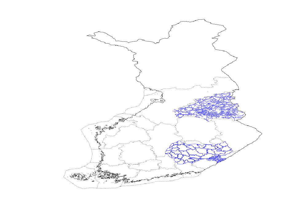 Figure 22
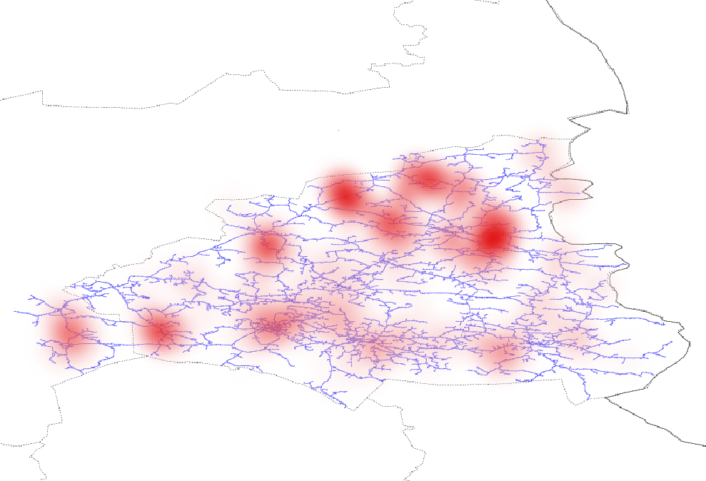 Figure 23
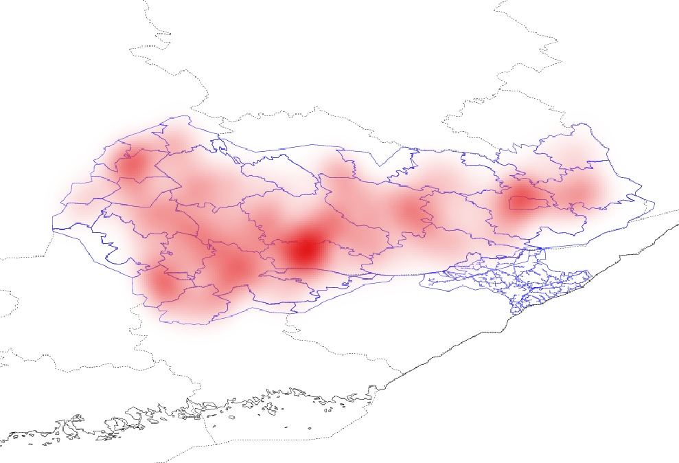 Figure 24
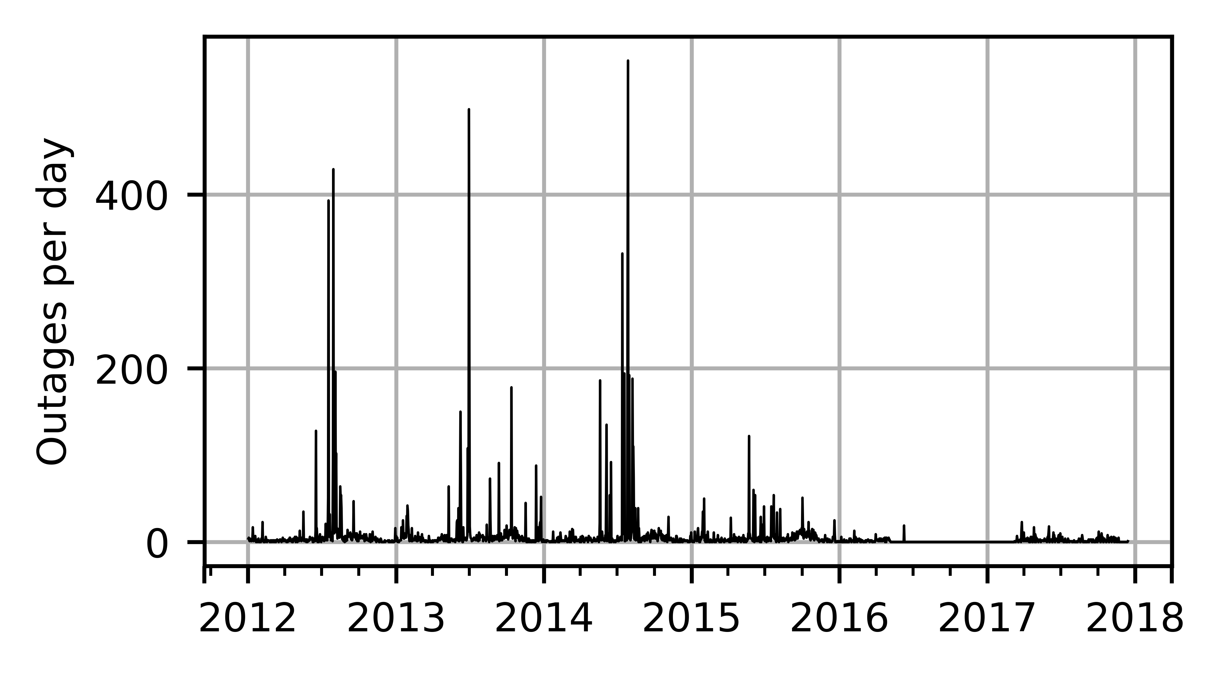 Figure 25
 Figure 26
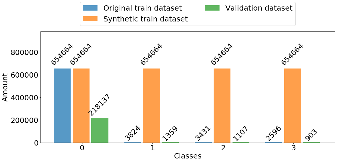 Figure 27
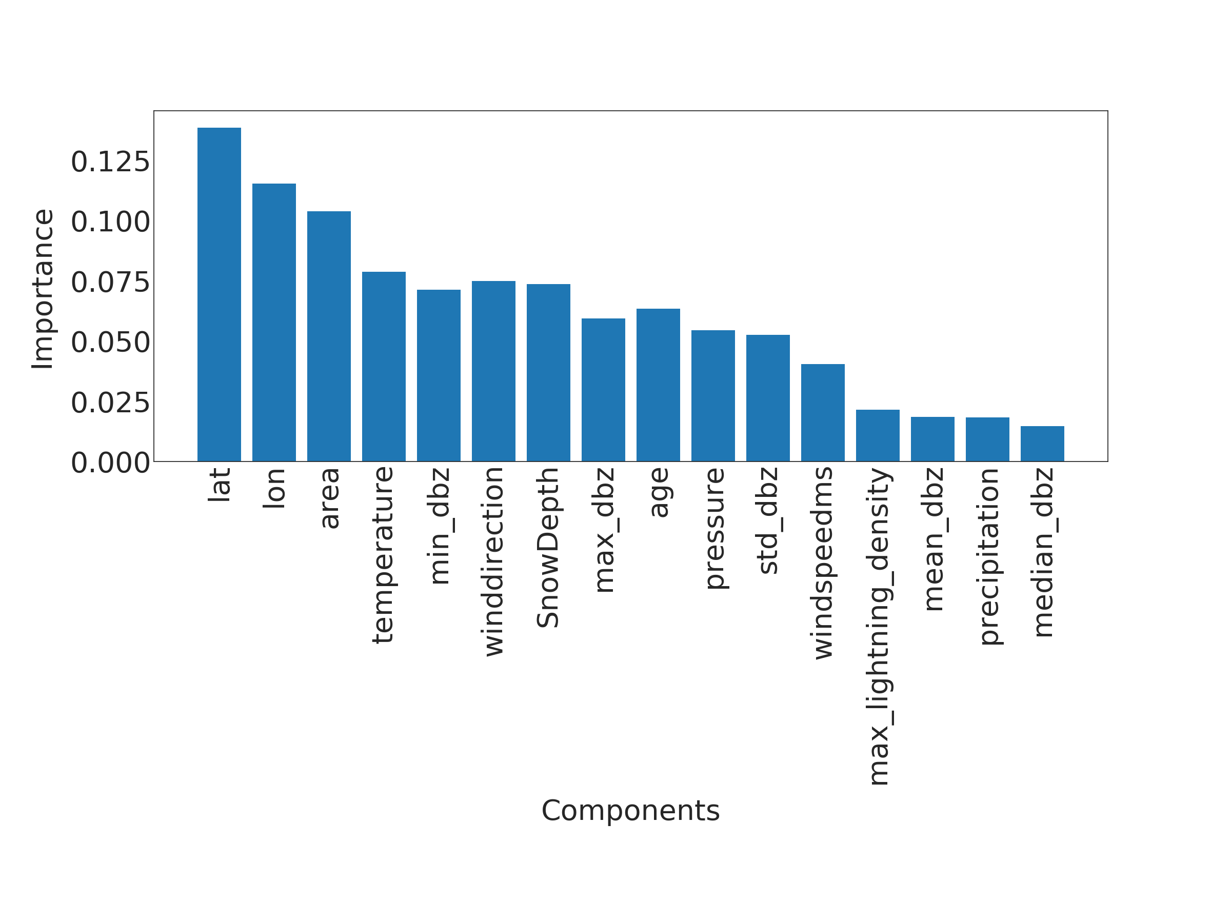 Figure 28
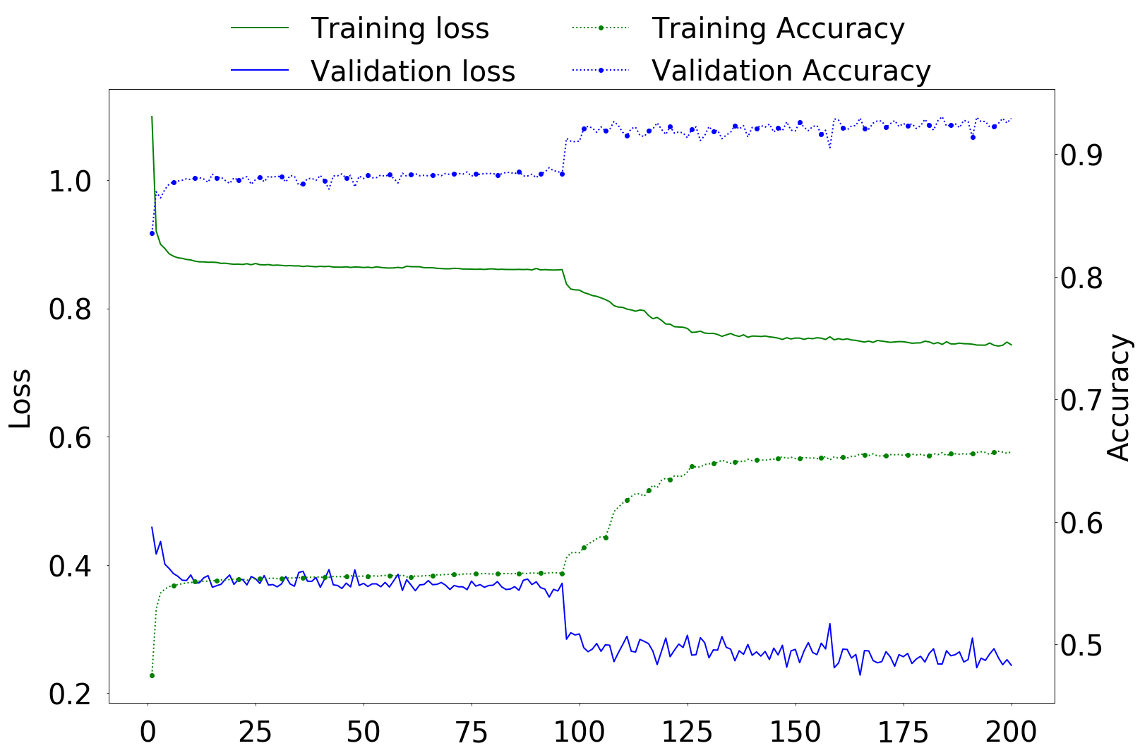 Figure 29
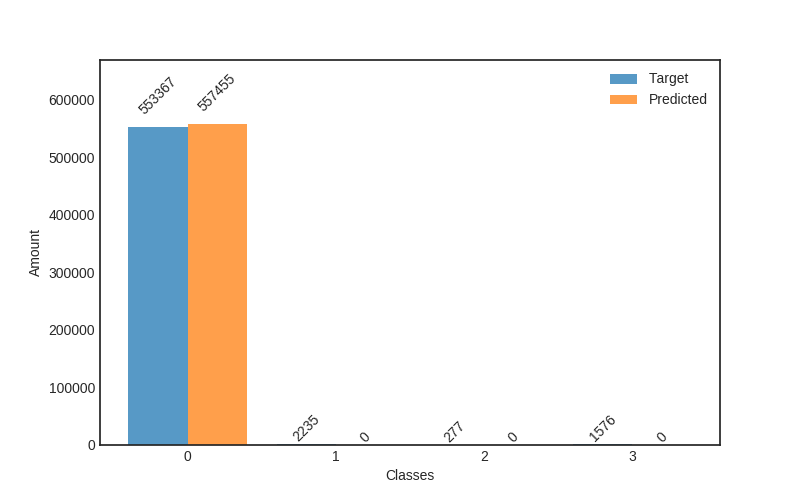 Figure 30
| Class | Share of transformers |
|---|---|
| 0 | no damage |
| 1 | 0 - 10 % |
| 2 | 10 - 50 % |
| 3 | 50 - 100 % |
| Feature | Explanation |
|---|---|
| Area | Area covered by the storm cell |
| Age | Age of the storm |
| Lightning density | Lightning density under storm cell |
| Max DBZ | Maximum radar reflectivity of the storm cell (spatially). Represents maximum rain intensity. |
| Min DBZ | Minimum radar reflectivity of the storm cell (spatially). Represents minimum rain intensity. |
| Mean DBZ | Mean radar reflectivity of the storm cell (spatially) |
| Median DBZ | Median radar reflectivity of the storm cell (spatially) |
| Std of DBZ | Standard deviation of radar reflectivity of the storm cell (spatially) |
| Lat | Storm center latitude |
| Lon | Storm center longitude |
| Temperature | Air temperature from ground |
| observations | |
| Pressure | Air pressure from ground |
| observations | |
| Wind speed | Wind speed from ground |
| observations | |
| Wind direction | Wind direction from ground |
| observations | |
| Precipitation amount | Precipitation amount from ground observations |
| Snow depth | Snow depth from ground |
| observations |
| Parameter | Value |
|---|---|
| Number of trees in the forest | 200 |
| Max depth | unlimited |
| Minimum nro. of samples to split | 2 |
| Minimun nro of samples to leaf | 1 |
| Features to consider for split | 4 |
| Max nro of leaf nodes | unlimited |
| Parameter | Value |
|---|---|
| Batch size | 256 |
| Epoch count | 1000 |
| Dropout probability | 10 % |
| (learning rate) | 0.001 |
| (exp decay for momentum) | 0.9 |
| (exp decay for momentum) | 0.999 |
| (stability constant) | |
| Initial decay | no decay |
| Metrics | MLP | MLP | RFC | RFC |
| Accuracy | 93 % | 85 % | 100 % | 98 % |
| AUC | 0.82 | 0.81 | 0.86 | 0.88 |
| Precision | ||||
| micro average | 93 % | 85 % | 100 % | 99 % |
| Precision | ||||
| macro average | 29 % | 31 % | 66 % | 67 % |
| Recall | ||||
| micro average | 93 % | 85 % | 100 % | 99 % |
| Recall | ||||
| macro average | 65 % | 67 % | 75 % | 79 % |
| F1 score | ||||
| micro average | 93 % | 85 % | 100 % | 99 % |
| F1 score | ||||
| macro average | 32 % | 34 % | 70 % | 72 % |
Peer Reviews
No public reviews on file for this paper yet. If you reviewed it on a platform where reviews are public (OpenReview, ICLR, NeurIPS, ICML), you can paste yours below so the community can read it here.
Videos
No videos yet. Explain this paper in a talk, walkthrough, or lecture? Add one.
© 2019 IEEE. Personal use of this material is permitted. Permission from IEEE must be obtained for all other uses, in any current or future media, including reprinting/republishing this material for advertising or promotional purposes, creating new collective works, for resale or redistribution to servers or lists, or reuse of any copyrighted component of this work in other works.
Short-term prediction of Electricity Outages Caused by Convective Storms
Roope Tervo, Joonas Karjalainen, Alexander Jung Manuscript received February 15, 2019; revised May 3, 2019 and May 31, 2019; accepted June 5, 2019. (Corresponding author: Roope Tervo.) Roope Tervo is with Finnish Meteorological Institute, Observing and information systems centre, B.O. 503, 00101 Helsinki, Finland (e-mail: [email protected]) Joonas Karjalainen is with Finnish Meteorological Institute, Observing and information systems centre, B.O. 503, 00101 Helsinki, Finland (e-mail: [email protected]) Alexander Jung is with Aalto University, Dept of Computer Science, B.O. 11000, 00076 Aalto, Finland Digital Object Identifier 10.1109/TGRS.2019.2921809
Abstract
Prediction of power outages caused by convective storms which are highly localised in space and time is of crucial importance to power grid operators. We propose a new machine learning approach to predict the damage caused by storms. This approach hinges identifying and tracking of storm cells using weather radar images on the application of machine learning techniques. Overall prediction process consists of identifying storm cells from CAPPI weather radar images by contouring them with a solid 35 dBZ threshold, predicting a track of storm cells and classifying them based on their damage potential to power grid operators. Tracked storm cells are then classified by combining data obtained from weather radar, ground weather observations and lightning detectors. We compare random forest classifiers and deep neural networks as alternative methods to classify storm cells. The main challenge is that the training data are heavily imbalanced as extreme weather events are rare.
Index Terms:
Radar tracing, Power distribution faults, Machine learning, Multilayer Perceptrons
I Introduction
A key problem faced by Finnish power grid operators is the prediction of damages caused by extreme weather events such as convective storms such as thunders which occur often in Finland during summer time [1]. These thunderstorms are typically geographically highly localised (50 km2) and have a short duration (less than 30 minutes) [2, 3] which makes them hard to detect and predict.
The damages produced by intense winds, lightning and tornadoes have significant social impacts and incur significant liability for power grid operators. Overhead lines which are still widely used in rural areas are particularly prone to weather events. During the year 2017, 78 percent of all outages were caused by extreme weather events; 50 percent of these outages are caused by strong winds, 45 percent by ice and snow load, 5 percent by lightning and rest by other weather events [4, p. 20]. Extreme weather events cannot be prevented but power grid operators can minimise the effect of weather-induced damages. For example, they can up-level workforce in relevant areas when bad weather is anticipated.
Since weather-caused damages incur a significant economic loss, a lot of effort has been put into studying efficient prediction of impacts of extreme weather events. Blackouts caused by large scale hazards such as hurricanes have been studied in e.g. [5, 6, 7, 8, 9, 10, 11, 12, 13]. In contrast, we focus on more localised phenomenons related to convective storms. The authors of [14] present an outage prediction method based on static areas and the authors of [15] ennoble this work to take power grid topology into account. [16] uses Random Forest Classifier to a regular grid to create power outage prediction. In [17], the authors compare a Poisson regression model and a Bayesian network model in the task of modelling failure rates in overhead distribution lines. These methods exploited data from ground weather stations and lightning detection network with a daily time interval. Kankanala et al. have experimented regression models [18] and multilayer perceptron (MLP) neural network [19] along with ensemble learning [20] to predict outages caused by wind and lightning in overhead distribution systems. Their methods are based on data from nearby weather stations. Bayesian outage probability (BOP) model predicting power outages has been discussed in [21]. They combined weather radar information from several sources to a geographically unified grid. Authors of [22] propose a method to forecast a probability that developing thunderstorm will produce severe weather. The method consists of creating spatial objects from satellite and weather radar data, tracking them and classifying them to be hazardous or non-hazardous with Naïve Bayesian classifier. The method is focused on predicting tornadoes, severe wind gusts, and hailstones and is aimed to provide a tool to weather forecaster. The problem of storm cell identification and tracking has been studied thoroughly also in [23].
We propose a novel method to predict the impact of severe convective storms on the power grid. Our method combines storm cell identification and tracking developed in [23] with state of the art machine learning techniques. The storm cell identification and tracking used in this work are related to [22]. However, [22] considers a binary classification for weather forecasters whereas we predict the short-term damage potential specifically for a power grid. Similar to [17, 18], we use data produced by weather stations and lightning detection network and combine them with parameters derived from weather radar data as used in [21]. Moreover, since our method is based on identified storm cells, we are able to use also parameters characterising the storm cell itself. This provides much more accurate spatial and temporal resolution than weather stations and more information about the whole storm instead of any individual point.
This paper is organised as follows: In Section II, we formulate a problem as a classification problem. In Section III we first discuss using an object-based approach in predicting power outages and propose two alternative classification methods of random forest classifier (RFC) and deep neural network classifiers to predict amount damage. Some illustrative numerical experiments based on historical data collected by the Finnish Meteorological Institute (FMI) are discussed in Section IV followed by results in Section IV-A.
II Problem Formulation
We model outage prediction as a supervised learning problem with occurred power outages as labels and weather conditions as features. Outage data and power grid description are fetched from two power grid operators. The data set contains in total of 33 858 outages. It is notable that actual damage may happen to any point in the power grid, but outages are always reported at nearby transformer nodes of the power grid. One physical damage may also turn down several transformers. Unbroken transformers can later be taken into use remotely by power grid operator (without repairing the actual damage). One physical damage can thus be reported as several outages in the power distribution network.
Spatial coverage of the data is shown in Fig. 2. Heatmaps of all outages recorded between 2012 and 2017 are shown in Fig. 3a. and 3b. It is notable that outages are not distributed evenly over the area. Instead, both areas contain “hotspots” where outages are more common than elsewhere. Outages also occur very unevenly in time. Fig. 4 shows amounts of outages per day in the whole area. One can see that most outages have happened during only a few days. It is also notable that although the worst peaks in outages get a place during summers, there are minor peaks also during winters. These outages are most probably caused by wet snow load on trees and wires [24]. The method considered in this paper is unable to address these cases.
We cast the problem of recognising a damage potential of the storm to as categorisation problem and propose two alternative methods for the task. In particular, we categorise storms into four classes based on how much damage they are expected to cause for the power grid during one time step. A storm at any given time step is defined as a “sample” in the remainder of this paper. The storm cells are assigned to a class based on how large share of transformers under the storm is without electricity. That is, a number of transformers in the whole network do not effect on the classification. We use four classes, described in Table I. The particular choice of these classes aims to provide a simple ’at glance’ view which is convenient for the end user (power grid operator).
The data are very imbalanced as most of the storm cells are not powerful enough to cause harm to the power grid. We depict a histogram of the target classes contained in the training data set in Fig. 6. In particular, we have 872 801 (98,5 %) samples of class 0 (no harm), 5183 (0.6 %) samples of class 1, 4538 (0.5 %) samples belonged to class 2 and only 3499 (0.4 %) belong to class 3 (most harmful).
III Proposed Methods
We used weather data collected by FMI during the years 2012 to 2017. Data are collected from weather radars, weather stations, and lightning detection. The data are pre-processed as introduced in [23]. First, we identify storm cells by contouring weather radar reflectivity composite constant altitude plan position indicator (CAPPI) images with a solid 35 DBZ threshold. The particular chosen threshold enables detecting full storm systems like multicellular storms [25, 26]. The radar images have 250 meters spatial resolution and 5 minutes update interval. Anomaly detection and removal with methods described in [27] has been applied to the radar images as part of FMI operational image processing. Contoured storm cells are stored as geographical objects into a PostGIS database.
After contouring, we apply the GDBSCAN method [28] (generalised form of DBSCAN [29]) to cluster the contoured objects. Within the DBSCAN method, a storm cell is considered as a core point if the area sum of its nearby storm cells exceeds the given area threshold. The storm cells that are within the neighbourhood of a core point (inside given radius) but do not fulfil the minimum area criteria are considered as outliers. Together with their outliers, connected core points form a cluster. Storm cells that do not fulfil the area criteria of core points and are too far from any core point are regarded as noise. In this study, the area limit was set to and the neighbourhood radius was set to . Different parameter values have previously been evaluated subjectively and used in [30].
After clustering, we track and nowcast movement of the storm cells using method originally introduced in [31]: first, we interpolate clusters of previous time step to the current time step using optical flow [32] with Lucas-Kanade method [33]. If interpolated and current time step clusters overlap over the required threshold, we consider them connected. Predicting movement of the storm cells is done by Kalman filtering based method introduced in [30]. The prediction is done for a time horizon of 2 hours ahead with a time resolution of 5 minutes. Every storm cell is identified with a globally unique identifier so that the whole lifecycle of the storms can be tracked. In particular, all overlapping storm cells in the same cluster are assigned with the same identifier. The unique identifier also makes the storms easily referable afterwards.
The pre-processing produces a training set where each sample is characterised by in total of 16 features listed in Table II and a target class based on the number of occurred outages. The features contain parameters fetched directly from 2-dimensional CAPPI radar images like area, age, and radar reflectivity (DBZ) parameters. The storm center is also taken into account because the characters of forest vary significantly in different parts of Finland. Several ground observations fetched from weather stations under storm path are used as well. Because the location of outage reports contains a lot of inaccuracy and devastating phenomenons such as wind and lightning may occur also outside the cluster area, ground observation and outage search area are extended by buffering storm geometry with 0.1 degrees.
Our overall process is described in Fig. 1. A novel approach of this work is to combine classification methods to identified and tracked storm cell clusters to create power outage prediction. Instead of predicting (predefined limits of) weather variables, we focus on the impact of weather and let the classification method to deduce relevant variables and limits. Applying classification to (clustered) storm cells instead of using predefined areas or grid-based methods provides more accurate spatial and temporal resolution. Moreover, we argue that handling storms as geographical objects allows us to better characterise damage potential. Implementing classification to clusters instead of individual storm cells enables capturing the whole life cycle of the storm system [34]. We also argue that classification instead of regression better captures areas of interest from power grid operator point of view.
We created two alternative methods for classification: Random Forest Classifier (RFC) [35] and multilayer perceptron (MLP) neural network [36]. Random forest classifier is an ensemble method which forms a decision tree based on randomly selected samples from train data. The method is reported to work well for the imbalanced data [37, 38] and is hence very interesting candidate for this particular application. For the training of the RFC, we used the Gini impurity as loss function, i.e.
[TABLE]
where is the number of classes and is the share of class in the tree.
As an alternative to RFC, we also implemented a classifier based on a multilayer perceptron (MLP) neural network [36]. The network structure, among hyperparameters, was searched by trial and error. The best solution we were able to find is described in Fig. 5. The first layer contains 20 nodes wide dense layer. In the following layers, the number of nodes is reduced to 16, 8, 4 and finally to 1 node. The first three dense layers use the rectified linear unit (Relu) as activation and dropout regularisation layers are included after first and second dense layers. In the final layer, we used the “Softmax” activation function in order to obtain the predicted class probabilities in the output layer. For MLP, we used the cross-entropy loss function [39]. This loss is defined as
[TABLE]
where is a probability distribution of true labels and is a probability distribution of predicted labels. Categorical entropy is a good default choice and it has an optional advantage that different classes can be easily preferred by giving different weights for the classes.
We combined the classifiers with the synthetic minority over-sampling technique (SMOTE) [40] to handle imbalanced data. The method generates new training samples in the vicinity of the original training samples by interpolating their nearest neighbours (in the feature space) as following:
[TABLE]
where is an original minority class sample, is one of ’s nearest neighbour and is random variable drawn uniformly from the interval . The synthetic data set generated by SMOTE contains data points with a balanced distribution of classes (see Fig. 6).
IV Numerical Experiments
We divided the data set into training and validation set with share of 75 % and 25 % respectively. SMOTE over-sampling was performed only for the training set. For RFC, optimal hyperparameters were obtained with random search cross-validation [41]. We used F1 macro average score for cross-validation so that all classes are valued equally in imbalanced data set. To be more specific:
[TABLE]
[TABLE]
[TABLE]
where is amount of true positive samples, false positives and false negatives in class . F1 scores of three best evaluation varied relatively much (0.70, 0.68 and 0.66) which indicates that the model is sensitive to the hyperparameters. The best obtained parameter set is listed in table III. The classification accuracy obtained for the training set was around 98 % and for the validation set up to 88 %. Thus, the RFC tends to slightly over-fit the training data.
One nice feature of RFC is that it provides relatively easy means to extract the importance of used features. The feature importance is plotted in Fig. 7. The importance analysis indicates that 12 out of 16 used features have significance in the classification. One can see that the storm center (latitude and longitude) are by far the most important features which makes sense as occurred outages are condensed at certain areas. It is also notable that the most important feature fetched from weather radar is an area of the storm, not the intensity of precipitation (DBZ). Several ground observations such as temperature, wind, pressure, and snow depth have relatively high importance as well. We tried to fit the method with a different number of features. While differences were small, the best results were nevertheless obtained with all 16 features.
Finding an optimal setup for the MLP network was a significantly more challenging task. Both network topology and hyperparameters were searched by trial and error. We started from one hidden layer and added more layers as long as they improved the results. For each round, we evaluated several different sizes for hidden layers with different activation functions. Training and validation loss and accuracy of the final training are plotted in Fig. 8. There is no sign of over-fitting and thus a quite low dropout probability was used for both dropout layers [39]. The batch size was a compromise to provide enough performance in sufficient time. We used the Adam optimiser [42] for training the model to avoid challenging points in the optimisation space. Final setup for hyperparameters is listed in table IV.
Data contained a large number of incomplete samples as capabilities of weather stations varies a lot. Absent parameters were initialised to zero to ensure technical coherence of the data. The intuitive assumption would say that filtering those samples would be beneficial to gain better results. We created a new data set from samples which contained all parameters and used that to train the classification methods. The new data set contained 563 571 samples (63 % of the original data set). Optimal hyperparameters for RFC with the new data set were re-optimised with random search cross-validation. For MLP, we used the same setup as for the full data set.
IV-A Results
The results are shown in table V. We evaluated performance with accuracy, Area Under the Curve (AUC) precision, recall and F1 score using both micro and macro average where applicable. The micro average is calculated from all samples from all classes. The macro average is calculated by taking an average of scores counted from each class independently. [43, p. 679]. To be more specific, having binary metrics where , and are amount of true positive, false positive, true negative and false negative samples respectively, one can define macro average as:
[TABLE]
and micro average as:
[TABLE]
where is amount of samples. Thus micro average is more suitable metrics for imbalanced data.
In the end, RFC performed better for predicting the amount of damage. Its accuracy and a micro average of precision, recall and F1 score were nearly 100 % (depending on used data set for training) but corresponding macro averages are significantly lower, varying from 66 to 79 %. Differences between micro and a macro average of used metrics are explained by dominating class 0 (no damage) in the data set. Performance for individual classes can be best seen in confusion matrices (Fig. 9. and 10). RFC is able to predict class 0 (no damage) with over 99 % accuracy and class 3 (most harmful) with 90 % accuracy but has troubles to distinguish classes 1 and 2 (68 to 59 % accuracy respectively). Precision-recall curves are plotted in Fig. 11. and 12. All models have extremely good precision (defined in equation 5) and recall (defined in equation 6) for class 0. Both RFC versions perform relatively well for class 3 but do not show proper skill for classes 1 and 2 having precision and recall mostly below 0.5. MLP works remarkably worse in terms of precision.
Impacts of filtering samples with missing values are two-pronged. Using clean data () for training improved the AUC and the macro average of precision, recall and F1 score but decreased accuracy a little bit. RFC trained with clean data set performed a little bit better with classes 1, 2 and 3 but worse with dominating class 0. That is to say, using clean data in training yielded to a little bit more false alarms but less missed cases. Nevertheless, the differences were marginal.
The results of the MLP classifier was significantly worse. While the MLP trained with full data set provided 93 % accuracy for class 0 and 77 % accuracy for class 3, accuracy for classes 1 and 2 are below 50 %. The MLP provided especially poor precision and F1 score giving a high false positive rate compared to true positive rate. Using the full data set for training yielded to better results than the clean data set with the MLP.
Classification is fast with both classifiers. For example, 221 506 samples can be classified in about 5 seconds with two 3,3 GHz i5 CPUs. While optical flow is a lightweight algorithm, DBSCAN method has a computational cost [29], which may be challenging during “active days”. Performing the clustering in under five minutes before the next radar image is produced requires significant computing power. Our experience is that at least 16 core server is required for processing area covering Finland.
V Conclusions
This paper studied the application of RFC and MLP classifiers to the problem of predicting power grid outages caused by hazardous storm cells. The classification method was based on characteristics of the storm cell extracted from CAPPI weather radar images, related ground weather observations, and lightning detection information.
Some illustrative numerical experiments based on weather data collected by FMI indicated that RFC can outperform deep MLP in predicting the amount of damage caused by storm cells. While MLP provided only poor performance, RFC showed very promising potential for the prediction task. Specially non-harmful and the most harmful cases were predicted with excellent accuracy.
This work suggests several interesting avenues for future research. Although used features already covered a quite wide range of environmental measurements, several promising but unutilised data sources still exist. Echo top information and speed of the storm could possibly give a good indication of its damage potential. Storm center seems to help the current classification method a lot but high importance of location prevents the method to be used in other areas without re-training it. The more generalised approach would maybe be to use the height of the forest as an input.
One promising direction is to use more advanced models and methods for the training data, e.g. times series models and recurrent neural networks. The time dimension could also be taken into account by adding ‘memory’ to the RFC so that predicted class of the storm is used as a feature for the prediction of following time step.
So far, we also used only very basic methods for coping with missing data (just replace by zero) and imbalanced training data (using SMOTE). Imputing missing data with kriging interpolation based methods (first introduced in [44]) would most probably improve the results. It would also be interesting to apply more advanced techniques for coping with imbalanced data, e.g. the “Rare-Transfer” algorithm [45].
Currently, Random Forest Classifier is used in an operational application.
Acknowledgements
The authors would like to thank the project partners Jä̈rvi-Suomen Energia, Loiste Sähkoverkko, and Imatra Seudun Sähkönsiirto for data and exprtice. Previous version of this work has been published as a conference paper [1].
The reference list from the paper itself. Each links out to its DOI / PubMed record.
- 1[1] Punkka Ari-Juhani and Bister Marja, “Occurrence of Summertime Convective Precipitation and Mesoscale Convective Systems in Finland during 2000 – 01,” Monthly weather review , vol. 133, no. 2, pp. 362–373, 2005.
- 2[2] E Galanaki, K Lagouvardos, V Kotroni, E Flaounas, and A Argiriou, “Thunderstorm climatology in the mediterranean using cloud-to-ground lightning observations,” Atmospheric Research , vol. 207, pp. 136–144, 2018.
- 3[3] G Brant Foote and Charles A Knight, “Results of a randomized hail suppression experiment in northeast Colorado. Part I: Design and conduct of the experiment,” Journal of Applied Meteorology , vol. 18, no. 12, pp. 1526–1537, 1979.
- 4[4] Esa Niemelä, “KESKEYTYSTILASTO 2017 (i),” Tech. Rep. 2018-06-14 11:51:52.916, Energiateollisuus Ry, Eteläranta 10, 00130 Helsinki, Finland, 2018.
- 5[5] Seth David Guikema, Roshanak Nateghi, Steven M. Quiring, Andrea Staid, Allison C. Reilly, and Michael Gao, “Predicting Hurricane Power Outages to Support Storm Response Planning,” IEEE Access , vol. 2, pp. 1364–1373, 2014.
- 6[6] Seth D. Guikema, Steven M. Quiring, and Seung Ryong Han, “Prestorm Estimation of Hurricane Damage to Electric Power Distribution Systems,” Risk Analysis , vol. 30, no. 12, pp. 1744–1752, 2010.
- 7[7] Roshanak Nateghi, Seth Guikema, and Steven M. Quiring, “Power Outage Estimation for Tropical Cyclones: Improved Accuracy with Simpler Models,” Risk Analysis , vol. 34, no. 6, pp. 1069–1078, 2014.
- 8[8] Seung Ryong Han, Seth D. Guikema, and Steven M. Quiring, “Improving the predictive accuracy of hurricane power outage forecasts using generalized additive models,” Risk Analysis , vol. 29, no. 10, pp. 1443–1453, 2009.