Narrow peaks of full transmission in simple quantum graphs
A. Drinko, F. M. Andrade, D. Bazeia

TL;DR
This paper investigates quantum graphs with degree-3 vertices, identifying conditions for full transmission and suppression, including narrow peaks caused by quantum interference, with potential applications in quantum device control.
Contribution
It introduces specific configurations of simple quantum graphs that exhibit narrow transmission peaks and suppression windows, advancing understanding of quantum interference effects in these structures.
Findings
Identified regions of full transmission and suppression in diamond and hexagonal graphs.
Discovered narrow peaks of full transmission due to constructive interference.
Analyzed series and parallel graph arrangements for controlled quantum transmission.
Abstract
This work deals with quantum graphs, focusing on the transmission properties they engender. We first select two simple diamond graphs, and two hexagonal graphs in which the vertices are all of degree 3, and investigate their transmission coefficients. In particular, we identified regions in which the transmission is fully suppressed. We also considered the transmission coefficients of some series and parallel arrangements of the two basic graphs, with the vertices still preserving the degree 3 condition, and then identified specific series and parallel compositions that allow for windows of no transmission. Inside some of these windows, we found very narrow peaks of full transmission, which are consequences of constructive quantum interference. Possibilities of practical use as the experimental construction of devices of current interest to control and manipulate quantum transmission…
Click any figure to enlarge with its caption.
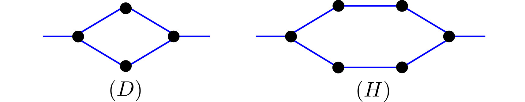 Figure 1
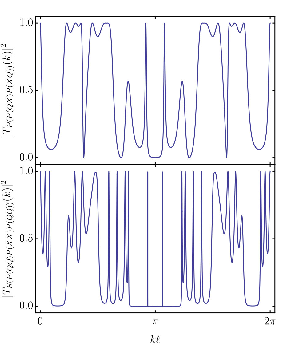 Figure 10
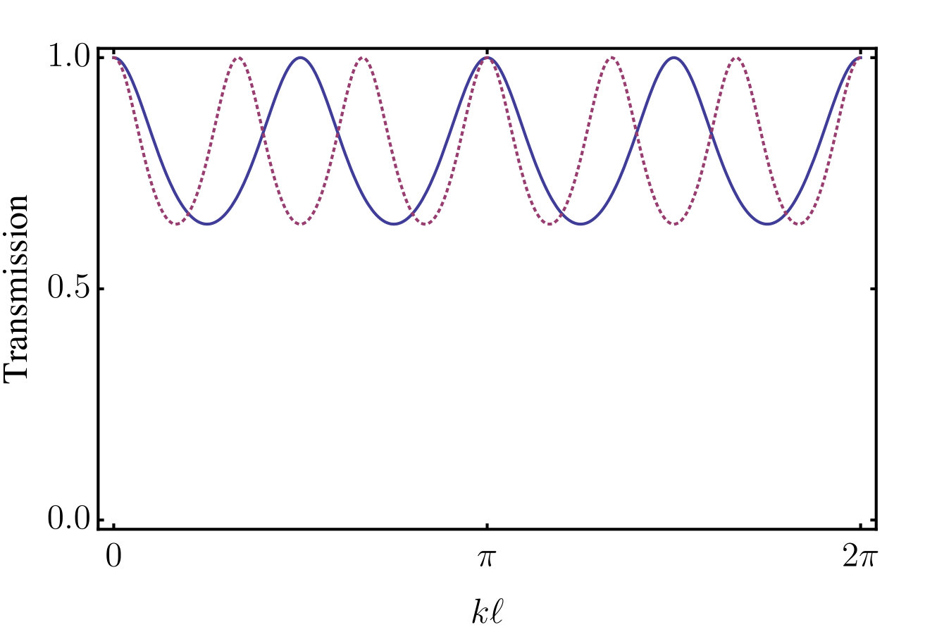 Figure 2
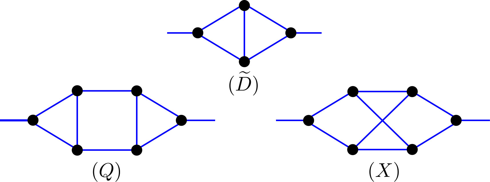 Figure 3
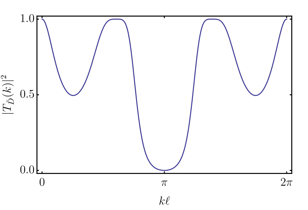 Figure 4
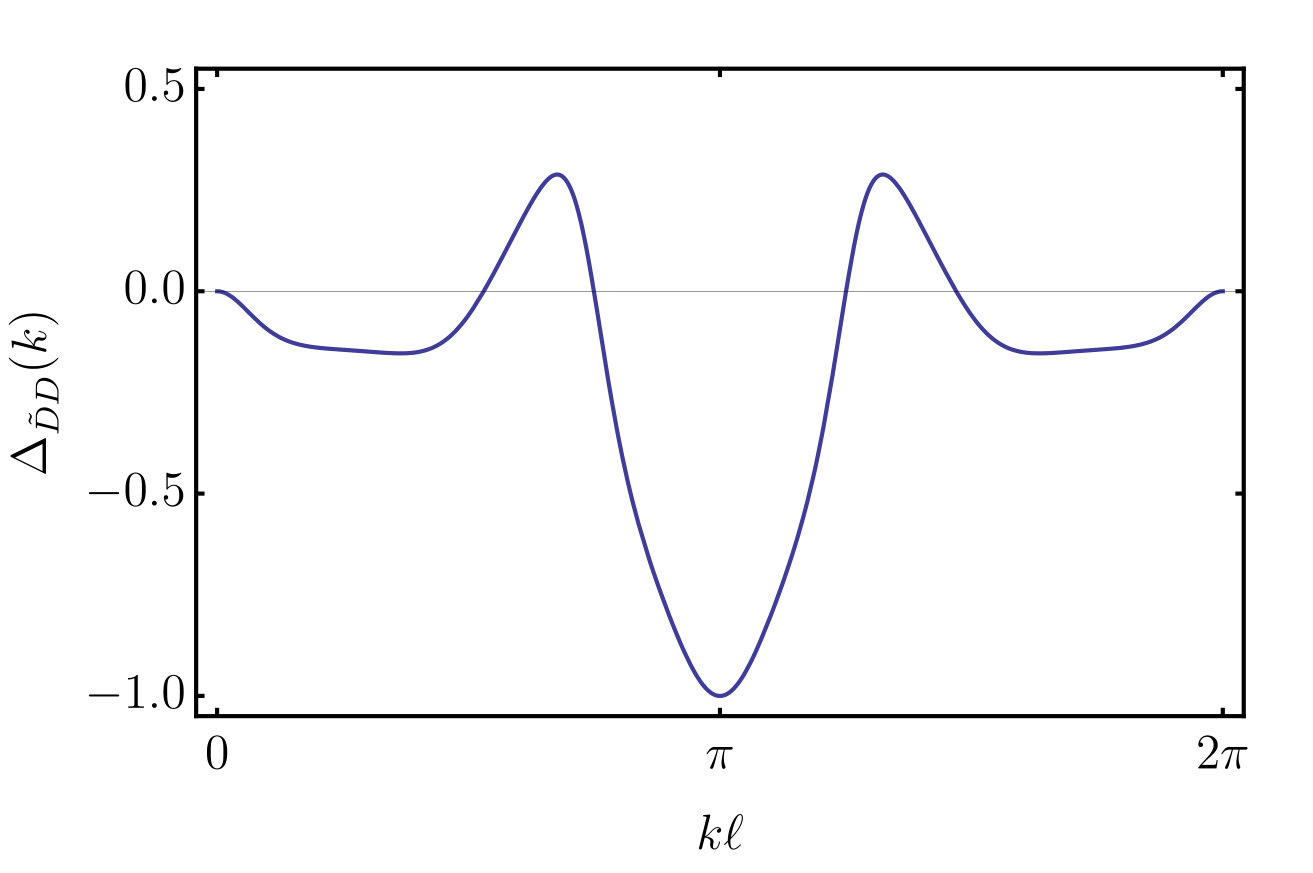 Figure 4
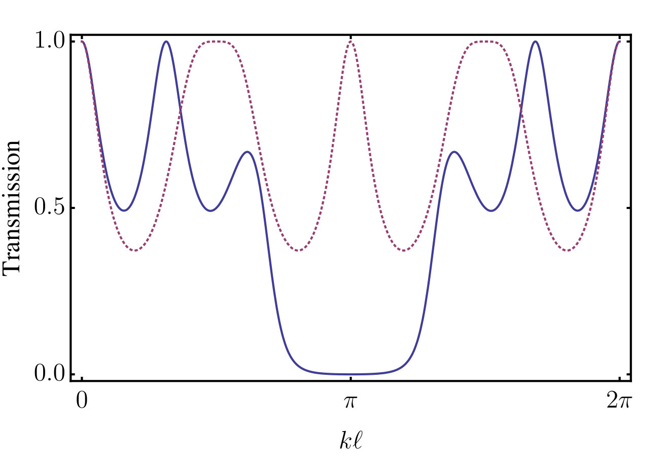 Figure 5
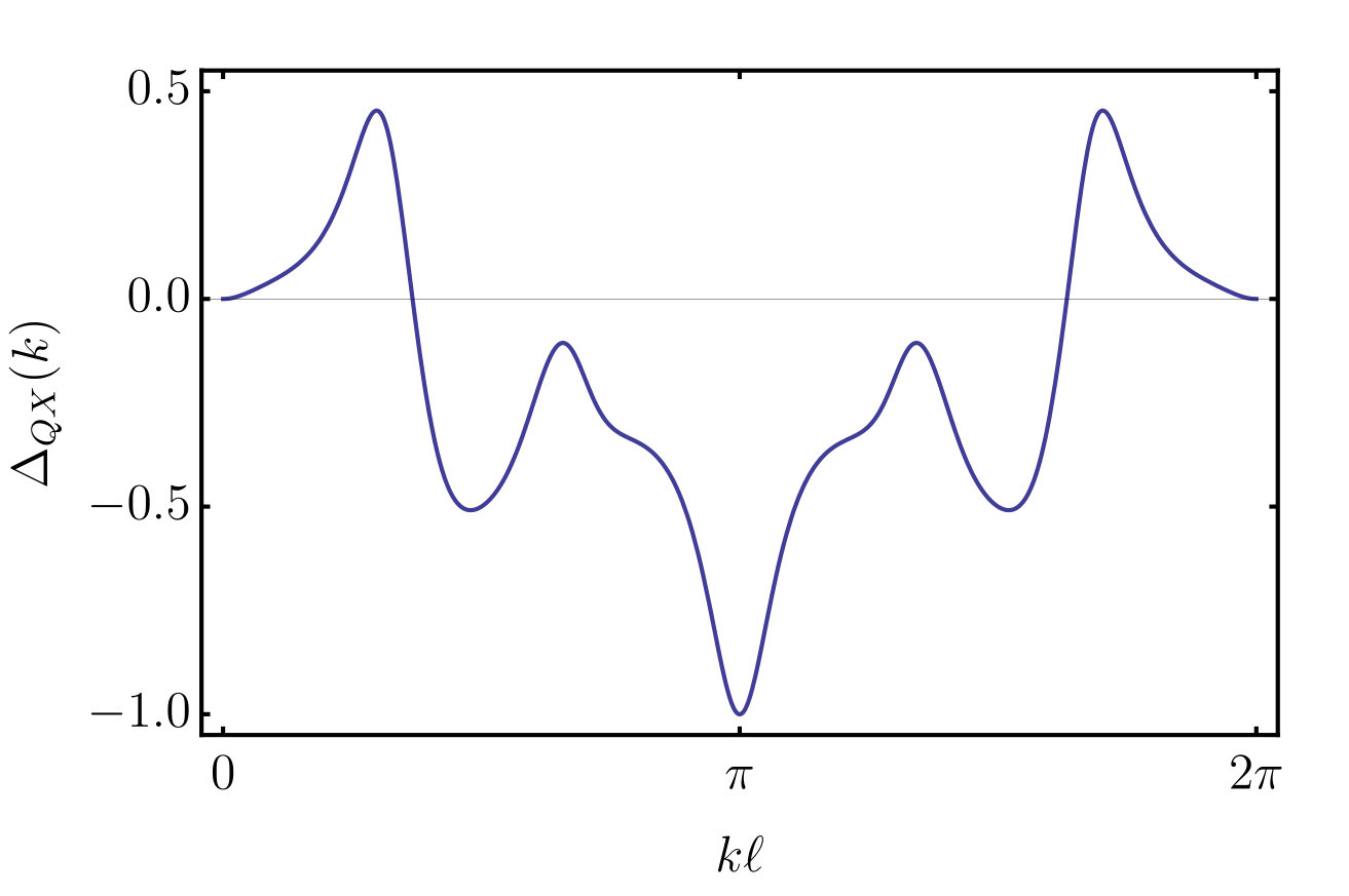 Figure 6
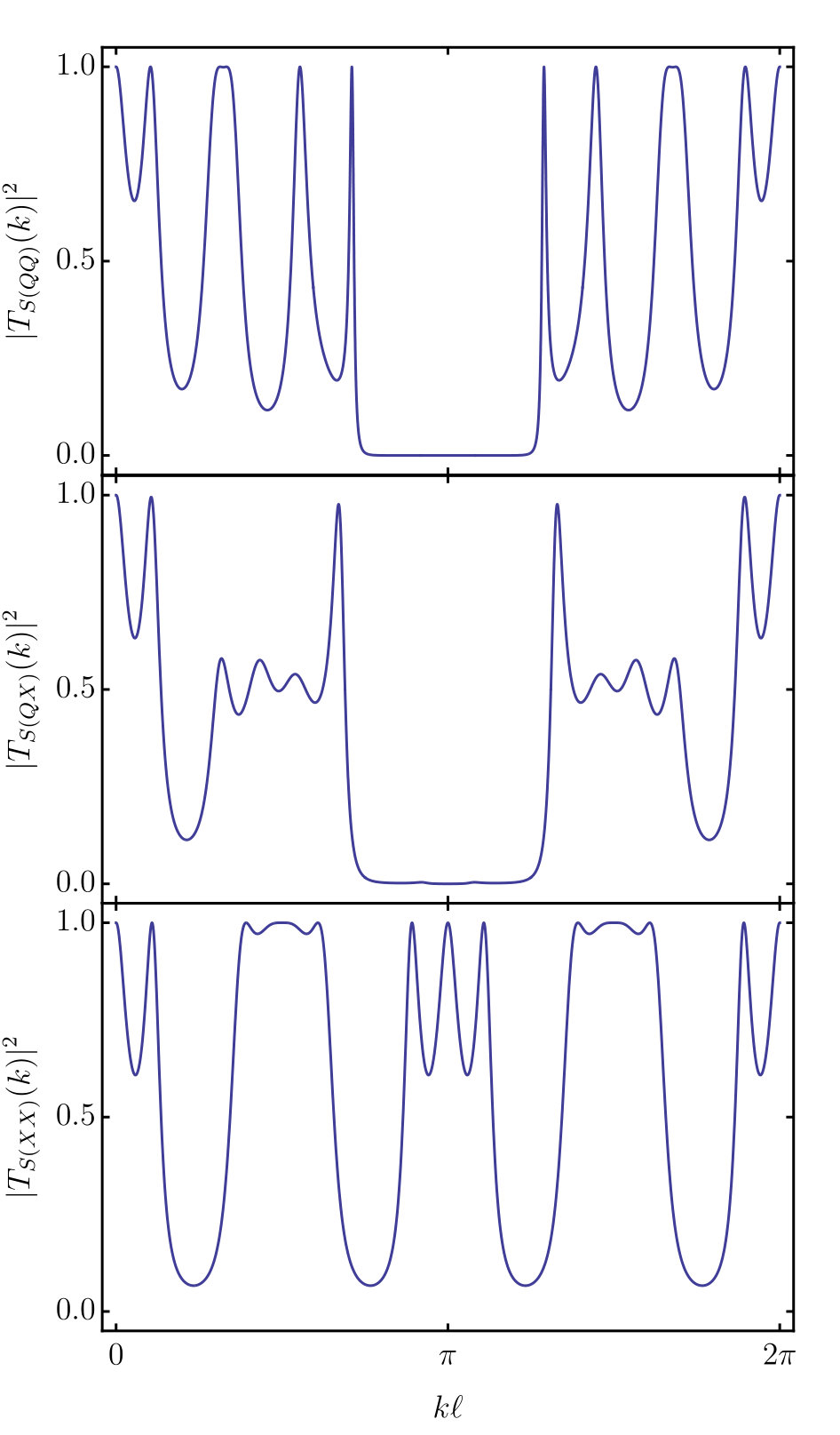 Figure 7
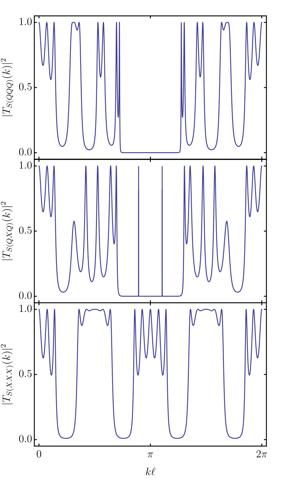 Figure 8
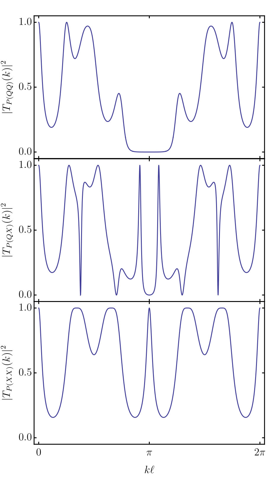 Figure 9
Peer Reviews
No public reviews on file for this paper yet. If you reviewed it on a platform where reviews are public (OpenReview, ICLR, NeurIPS, ICML), you can paste yours below so the community can read it here.
Videos
No videos yet. Explain this paper in a talk, walkthrough, or lecture? Add one.
Narrow peaks of full transmission in simple quantum graphs
A. Drinko
Programa de Pós-Graduação em Ciências/Física, Universidade Estadual de Ponta Grossa, 84030-900 Ponta Grossa, PR, Brazil
F. M. Andrade
Programa de Pós-Graduação em Ciências/Física, Universidade Estadual de Ponta Grossa, 84030-900 Ponta Grossa, PR, Brazil
Departamento de Matemática e Estatística, Universidade Estadual de Ponta Grossa, 84030-900 Ponta Grossa, PR, Brazil
D. Bazeia
Departamento de Física, Universidade Federal da Paraíba 58051-900 João Pessoa, PB, Brazil
Abstract
This work deals with quantum graphs, focusing on the transmission properties they engender. We first select two simple diamond graphs, and two hexagonal graphs in which the vertices are all of degree 3, and investigate their transmission coefficients. In particular, we identified regions in which the transmission is fully suppressed. We also considered the transmission coefficients of some series and parallel arrangements of the two basic graphs, with the vertices still preserving the degree 3 condition, and then identified specific series and parallel compositions that allow for windows of no transmission. Inside some of these windows, we found very narrow peaks of full transmission, which are consequences of constructive quantum interference. Possibilities of practical use as the experimental construction of devices of current interest to control and manipulate quantum transmission are also discussed.
I Introduction
In the past 20 years, quantum graphs Kottos and Smilansky (1999); Gnutzmann and Smilansky (2006) have been used to describe the behavior of quantum particles in idealized physical networks. The interest is due to the richness of the subject, which can be related to a variety of issues in physical and mathematical sciences. For instance, it has been simulated experimentally in microwave networks Hul et al. (2004) and it is also possible to synthesize quantum nanowire networks Dick et al. (2004); Heo et al. (2008). From the fundamental point of view, quantum graphs have became a test bed for studying different aspects in quantum mechanics and, due to the complex nature of the problem, the development of a unique method that holds for all graphs is difficult. Fortunately, however, there are some techniques developed in the literature that are able to deal with this problem Berkolaiko and Kuchment (2012). Among the several methods to deal with quantum graphs, an interesting one is the Green’s function approach, first proposed in Schmidt et al. (2003) and further explored in Andrade et al. (2016); Andrade and Severini (2018). In this work we shall deal with specific scattering properties of quantum graphs, which are identified by two leads and sets of vertices and edges, to be described in the next section. The focus is mainly on the transmission properties of simple graphs, owing to the possibility of applications of physical interest. We investigate the global transmission amplitude of quantum graphs as a function of the wave number of the incident signal using the Green’s function approach developed in Andrade et al. (2016); Andrade and Severini (2018). In particular, closer attention is given to the search for a new effect, which somehow remind us of the Braess paradox Braess (1968), and to the possibility to identify regions of wave numbers where the transmission coefficient increases significantly. The study will lead to the identification of peaks of quantum interference of very narrow width, similar to Feshbach resonances Feshbach (1958), in distinct arrangements of the basic structures to be studied in this work.
As one knows, the Braess paradox was first discussed by Braess in 1968 Braess (1968), and further studied in Refs. Braess et al. (2005); Youn et al. (2008). Originally, it showed that adding an extra road to a congested road traffic network to improve traffic flow may sometimes have the reverse effect, impeding the flow. The paradox was also discussed in several other contexts Pala et al. (2012); Sousa et al. (2013); Cohen and Horowitz (1991); Penchina and Penchina (2003); Barbosa et al. (2014), in particular in Pala et al. (2012), in which the quantum transport in mesoscopic networks with two and three branches revealed the transport inefficiency, confirmed by a scanning-probe experiment using a biased tip that modulates the conductance variation in terms of the tip voltage and position. It also appeared in Sousa et al. (2013) in a quantum ring of finite width, and in Barbosa et al. (2014) in the context of two quantum dots that are coupled together. Besides exploring global transmission properties of quantum graphs, we also concentrate on the presence of very narrow peaks of full transmission. The narrowness of the peaks reminds us of Feshbach resonances Feshbach (1958), which, in the context of quantum graphs, were investigated before in Ref. Waltner and Smilansky (2013) in a ring graph with edges with unequal sizes. Motivated by the above reasonings, in this work we follow the interpretation that the addition of a new path may under specific conditions enlarge the complexity of the system, opening new possibilities that may include unexpected responses. The effects that we are interested here appear in the search for the global transmission related to simple quantum graphs in the presence of quantum interference.
The investigation deals with quantum graphs, but in this work we consider simple graphs that are formed by arrangements of ideal leads, edges and vertices. This means that neither the vertices nor the leads and edges allow for vanishing of the quantum probability and, in this sense, any linear arrangement of leads, edges and vertices is trivial, since it gives full global transmission (see below). To go further on out of the trivial situation, we have to consider the possibility of a vertex being connected by a triple junction, in the form of a Y-shaped configuration, which is usually called a vertex of degree 3. In this case, the signal reaching a vertex has the possibility to reflect and return, and two possible paths of transmission, and this introduces nontrivial quantum effects that can appear in the global transmission coefficient of the graph. Of course, there is a diversity of possibilities of constructing graphs with vertices connected by two, three, four and more edges, and so in this work we consider the two simple possibilities of diamond and hexagonal arrangements. In the hexagonal case, we pay special attention to two arrangements, composed of two leads, six vertices and eight edges, with all the vertices having degree 3. We consider the hexagonal graphs in order to eliminate effects that could appear due to the presence of vertices with higher degrees, which seem to prefer backscattering Harrison et al. (2007). We call this the degree 3 condition, and use it to simplify the current investigation. The presence of vertices of degree 3 leads us to two distinct graphs that can be used to build arrangements that gives interesting responses, which can be of practical use in the construction of simple devices with important quantum properties. The two graphs to be considered in this work are hexagonal graphs with some internal structure, and this will also be of current interest, since hexagons are important to tile the plane to lead to hexagonal structures with vertices of degree 3, which are important part in nanotubes Saito et al. (1998) and in graphene sheets Neto et al. (2009); Gilje et al. (2007).
In order to deal with the above issues and implement the investigation, we organize the work as follows. In the next Sec. II, the main properties of quantum graphs are described, and there one concentrates mainly on the global transmission of simple graphs via the Green’s function approach. In Sec. III we introduce some simple graphs and describe and compare their global transmission coefficients. This investigation allows that we identify another effect, which is periodic and appears under the presence of quantum complexity. Also, in Sec. IV we deal with some simple composition of two distinct graphs and study some simple series and parallel arrangements of them. This will lead us to the presence of narrow peaks of full transmission, so in Sec. V we further investigate the issue to search for the presence of very narrow peaks of quantum interference. In Sec. VI we end the work, adding some comments and conclusions, paying further attention to the possibility of using the results of the work to applications of current interest to quantum transport.
II Procedure
In this section, we review some concepts of graphs as used in this paper. In particular, we deal with quantum effects and the use of the Green’s function approach for the calculation of the global transmission properties of quantum graphs, paying closer attention to the case of graphs with simple arrangements of leads, edges, and vertices.
II.1 Quantum graphs
A graph consists of a set of vertices and a set of edges Diestel (2010). The graph is described in terms of the adjacency matrix of dimension where the th element is defined by
[TABLE]
The degree of a vertex is defined as . We denote the set of neighbors of a vertex by and the set of neighbors of but with the vertices excluded by . A metric graph is a graph in which it is assigned a positive length to each edge. When a single ended edge is taken as semi-infinite (), it is called a lead. A quantum graph is a metric graph in which is possible to define a Schrödinger operator along with appropriated boundary conditions at the vertices Gnutzmann and Smilansky (2006). In general, the Schrödinger operator along the edge has the form
[TABLE]
where is the corresponding potential. In this sense, we can model distinct edges with the inclusion of different potentials; in particular, one can add a square well which will modify the transmission through the edge and so the global transmission through the graph. In this work, however, we shall take , that is, we shall use the free Schrödinger operator.
II.2 The Green’s function approach
In the context of quantum graphs, the exact scattering Green’s function for a quantum particle of fixed energy , with initial position in the lead and final position in the lead , is given by a sum over all the scattering paths connecting the points and , where each path is weighted by the product of the scattering amplitudes gained along the path Andrade et al. (2016). The reflection and transmission amplitudes, and , at the vertex , are determined through the boundary conditions defined at the vertex . With the help of the adjacency matrix of the graph, it was shown in Andrade and Severini (2018) that this sum over the paths can be written in the form
[TABLE]
where
[TABLE]
is the transmission amplitude. The is the family of paths between the vertices and , which are given by
[TABLE]
with . The family is given by the same expression above, but with the swapping of indices and . Then, in each vertex we associated one for every . In this work, we shall employ the above approach to determine the transmission coefficient for different quantum graphs and then discuss their properties. A useful quantity in our discussion is the difference between the transmission coefficients of two quantum graphs, and , and will be represented by
[TABLE]
Here, we shall consider equilateral quantum graphs where the length of all the edges are the same and set them to , such that .
II.3 The quantum amplitudes
Let us now discuss the possible boundary conditions. As one knows, a common vertex condition used is the so-called -type condition defined by Exner (1995)
[TABLE]
where is the value of the wave function at the vertex and is a real parameter related to the strength of the -type interaction. The prime in (II.3) represents the derivative, which should be taken in the outgoing direction, i.e., from the vertex into the edges or leads. Using this boundary condition the quantum amplitudes have the form Andrade and Severini (2018); Andrade et al. (2016)
[TABLE]
Among the choices for the value of , an interesting one is . In this case, we are considering no barrier at the vertices, resulting in the so-called Neumann-Kirchhoff boundary condition. As a result, the quantum amplitudes have the property of being independent of ,
[TABLE]
showing that the reflection amplitude increases with the increase of the degree of the vertex. When a Neumann-Kirchhoff boundary condition is used at a vertex of degree 2, the transmission amplitude is equal to 1 and the vertex becomes an ordinary point joining the edges. Such vertices are called Neumann vertices Gnutzmann and Smilansky (2006). In what follows, we shall adopt vertices of degree 3 with the Neumann-Kirchhof boundary condition. In this case the reflection and transmission amplitudes are explicitly given by and , respectively.
With the above conditions, we shall then be considering quantum graphs with ideal leads and edges, and with vertices that obey the Neumann-Kirchhoff boundary conditions. This is the simplest possibility, and we shall mainly consider vertices of degree 3, to avoid accounting for effects due to vertices of different degrees.
III Simple graphs
Let us now concentrate on simple graphs. One uses the symbol to represent vertices, and straight line segments to stand for the edges and leads, and first considers the graph {\color[rgb]{0,0,1}-}{\!\bullet\!}{\color[rgb]{0,0,1}-} with two leads – one at the left and the other at the right of the vertex. As we have already commented, this is trivial and gives |T_{{\color[rgb]{0,0,1}-}{\!\bullet\!}{\color[rgb]{0,0,1}-}}(k)|^{2}=1, since we are considering a Neumann vertex. If we go further and consider the graph {\color[rgb]{0,0,1}-}{\!\bullet\!}{\color[rgb]{0,0,1}-}{\!\bullet\!}{\color[rgb]{0,0,1}-} we also get full transmission, |T_{{\color[rgb]{0,0,1}-}{\!\bullet\!}{\color[rgb]{0,0,1}-}{\!\bullet\!}{\color[rgb]{0,0,1}-}}(k)|^{2}=1. In view of this, we have to consider vertices with higher degrees leading to more complex graphs to open the possibility of having nontrivial transmission effects, so we depict the diamond () and the hexagonal () graphs that are shown in Fig. 1. In this case, the transmission amplitudes can be written as
[TABLE]
and the corresponding transmissions coefficients are shown in Fig. 2.
The transmission coefficients are no longer nontrivial, and the effects are due to the presence of the left and right vertices of degree 3. Here we notice that since we are considering Neumann vertices, the difference between the diamond and hexagonal graphs depicted in Fig. 1 is only due to the difference between the two internal paths, which is at the ratio , as it nicely appears when one accounts for the difference between the periodicity of the transmission of the diamond and the hexagonal graphs that appear in Fig. 2.
Since the presence of vertices of degree 3 induces nontrivial transmission, we then focus on this and consider the new graphs which are depicted in Fig. 3. They are all constructed with vertices of degree 3 in the diamond and hexagonal families. Since there is only one graph in the diamond family, we cannot compare the transmission behavior of two distinct diamond graphs with vertices of degree 3. However, if we relax the degree 3 condition and consider the two diamond graphs that are depicted in Figs. 1 and 3, we see that the diamond graph of Fig. 3 has an extra edge which is not present in the diamond graph of Fig. 1, so it seems that the transmission through it would always be greater than the other one, which was already calculated above. To see how this works, we calculate the transmission coefficient of the graph, which is given by
[TABLE]
We then depict the difference in Fig. 4 and the result shows that the transmission through is not always greater than the one through . The effect shows that the addition of an extra edge in the graph to make it the graph, does not always improve the transmission probability. We believe that this is a manifestation of the quantum complexity that appears in the graph. However, since the two graphs and have different numbers of edges, and vertices with different degrees, we cannot separate how these effects contribute to the final transmissions. Due to this, from now on we concentrate on the transmission coefficient of the two graphs and of the hexagonal family that are depicted in Fig. 3 to compare their properties. We stress that all the vertices of these two hexagonal graphs have degree 3 and, also, they have the same number of edges and vertices. This means that our results will be contaminated neither by effects of vertices of different degrees nor by effects of different number of vertices and edges. The transmission amplitudes for these two graphs are given by
[TABLE]
and the corresponding transmission coefficients are displayed in Fig. 5, unveiling interesting nontrivial properties which we discuss below.
As we noted, the two transmission coefficients are periodic so we display them in Fig. 5 for the wave number in the interval of periodicity of the graph. We also observe that the transmission coefficient of the graph is more complex than the other one. More importantly, it may vanish in a large interval which we call the suppression band, inside its interval of periodicity. The results also show that there are regions in space, where the transmission is more or less significant for the than the graphs. That is, may be greater or smaller than , depending on the interval in space in consideration.
These results open the possibility to study the presence of an effect that is similar to the one that appeared above, with the two diamond graphs, but now with the vertices with the same degree. Here we depict the difference between the two coefficients, to see regions where one is higher than the other. This is shown in Fig. 6, and we can observe that for in the interval the transmission of the graph is higher than the transmission of the graph. However, for and for one sees that the transmission for the graph is greater than the one for the graph, and this is a manifestation of the quantum complexity related to these two graphs. In regard to the numerical results, all of them were obtained using the commercial Mathematica software by using standard techniques with precision of twelve decimal digits, and we decided to use only five digits in the final results.
To get further insight on the result depicted in Fig. 6, let us now briefly discuss the transmission of the signal at the classical level: one supposes that a classical signal enters the graph at the left (right) lead and leaves it at the right (left) lead; one notices from Fig. 3 that for the graph the shortest trajectory requires three steps, and that there are two distinct possibilities; for the graph, the shortest trajectory also requires three steps, but now there are four distinct possibilities. This suggests that the classical flux through the graph seems to be more efficient than the other one. However, the problem is more complex than this, because of the presence of reflection at the vertices. For instance, the next shortest trajectory for the graph requires four steps, and there are four possibilities; for the graph there is no trajectory with four steps. In fact, the graph has only trajectories with odd number of steps, whereas the graph has both even and odd number of steps. Thus, even classically, it is hard to decide which of the two graphs is more efficient to transmit the signal. At the quantum level the problem is harder, because of the quantum interference, and the result displayed in Fig. 6 shows that the answer depends on the wave number. Since the two graphs have the same number of edges and vertices and all the vertices have degree , it is the topological difference between these two graphs that leads to different transmission coefficients, which depends on the wave number and the quantum complexity involved in the problem.
The result in Fig. 6 suggests that both the and graphs are complex enough to give rise to other effects of current interest. They then motivate us to go further and explore other possibilities. In the current investigation we explore the fact that the graph engenders a band of no transmission in space, as it is easily identified from the blue solid line depicted in Fig. 5. This is the suppression band, and it is an interesting quantum effect that can be used in different applications. The simplest possibility is to use it to block the passage of a signal through the quantum graph, which can be seen as a device of direct interest to the construction of tools that allow for the control and manipulation of quantum transmission probability. Yet more interesting is to see the two quantum graphs as two independent quantum devices, which can be used for the construction of others, composed devices, and this will be investigated in the next section.
IV Graph circuitry
Let us now use the two quantum devices, the and the graphs, to build compound structures and study their transmission properties in light of the above investigation.
IV.1 Simple series circuits
We first consider the series composition, of the forms , , , and , where indicates the series composition of the graph with the graph , keeping the degree 3 condition of the vertices, which in the series arrangement occurs very naturally. We then calculate and display the transmission coefficient for all the cases in Fig. 7. Although the square and crossed graphs are different, the compound transmission does not depend on the order one chooses each other, so we say that . We compare the transmission displayed with the blue solid line in Fig. 5 with the one in the top panel in Fig. 7 to see that the series composition of two square graphs enlarges a bit the suppression band in space around , so it is a bit more efficient to block the passage of a signal. On the other hand, the violet dotted line that appears in Fig. 5 and the bottom panel in Fig. 7 show the appearance of extra maxima in the transmission coefficient of the graph. This composition also deepens the main minima, approaching them to suppression. The composition which appears in the middle panel in Fig. 7 is also interesting: it shows an almost invisible substructure in the suppression band, and this suggests that we further explore this effect.
To do this, we add another basic device to the series structure, so we consider compound structures with three devices. In this case there are several possibilities and in Fig. 8 we depict the three series arrangements , and , which are important for the considerations that follow below. The top and bottom panels in Fig. 8 show a behavior which appeared before, when we compared with Figs. 5 and 7. In particular, in the top panel in Fig. 8, one sees that the transmission coefficient vanishes completely in some interval in space, so we can also use this in applications of current interest. Moreover, the behavior that appears in the middle panel in Fig. 8 reveals an interesting quantum behavior – the presence of two very narrow peaks of full transmission inside the suppression band. They are very interesting and are consequences of the constructive quantum interference in the underlying graph, which we further study in Sec. V.
IV.2 Simple parallel circuits
Let us now study the case of parallel circuits. Here the condition that we only have vertices of degree 3 selects some specific combinations of the elementary devices. The simplest parallel possibilities are the , and structures, where is used to indicate parallel arrangements. The arrangement, for instance, is constructed as follows: one puts the graph on top of the graph, without contact, and at the center of the vertical arrangement, at the left and right one adds two extra vertices, the one at the left (right) being connected with a left (right) lead, and then connected with two other edges to keep the degree 3 condition, one going up to the graph, and the other going down to the graph.
We study the three distinct possibilities and in Fig. 9 we depict the transmission coefficients for the three distinct cases. We note that both the top and bottom figures give results somehow similar to the respective cases in the series arrangements shown in Fig. 7; compare the top results and the bottom results of both Figs. 7 and 9. However, the middle panel which describes the possibility is different from the case displayed in the middle panel of Fig. 7, so we go further and study other compositions.
IV.3 Other arrangements
The above results suggest that we study other possibilities. The series and parallel arrangements are more intricate than the elementary and compositions, and they require more complicated numerical calculations. However, if one keeps the condition of vertices of degree 3, there are several possibilities and we can, for instance, consider the parallel structures , and in parallel and in series. Examples are the cases , and , which represent parallel arrangements of parallel arrangements, etc., and , which represents a series arrangement of three parallel arrangements, etc.
We have studied several cases and, in comparison with the previous results, we found no qualitatively different behavior. To exemplify the findings, let us consider for instance the case of a parallel composition of two parallel compositions and a series composition with three structures of two parallel compositions. The results are depicted in Fig. 10, for the cases and , respectively. We note that the transmission coefficients for these new compositions add no different qualitative effects, in comparison with the previous results, so we end the calculations of transmission coefficients here.
V Interference
We see, from the transmission coefficients of the several arrangements already studied, the appearance of peaks of full transmission in the region around the center () of the periodic region in space, which we now want to investigate more carefully.
We first focus on the central peak that is displayed with the violet dotted line in Fig. 5. We do this by looking at the poles of the Green’s function which, for the graph depicted in Fig. 3, are all contained in the roots of the denominator of Eq. (15) Andrade et al. (2016). Here we identified a pole at , so one extends the investigation to the complex plane to find that this pole has a width that measures . Similarly, we also confirmed the presence of the pole at in the bottom panel in Fig. 7, but now the width is .
The more interesting case appears from the middle panel in Fig. 8 and in the bottom panel in Fig. 10. There are two similar peaks which engender very narrow widths, so we further examine the corresponding Green’s function and find the two poles that appear in the middle panel in Fig. 8: they are located at , and have very narrow width, which obeys . They are peaks of full transmission that appear inside the band of full suppression, and can be interpreted as peaks of constructive quantum interference. A similar situation appears in the bottom panel in Fig. 10. The presence of the two peaks symmetrically located around is a consequence of the time reversal symmetry of the quantum graphs, which does not distinguish the signal entering from the left (right) and leaving to the right (left). Note that the time reversal symmetry is present in all graphs here studied; it shows that , for , for all the global transmission coefficients.
VI Discussion
In this work we studied global transmission properties of some simple quantum graphs. We started with diamond and hexagonal graphs and, in the diamond family of graphs, we compared the transmission coefficients associated with the and arrangements that are depicted in Figs. 1 and 3. The difference between the two transmissions appears in Fig. 4, showing that it can be positive or negative, depending on the wave number of the incoming signal. For the and graphs, however, the degree of the vertices and the number of edges are not the same, so we moved on to the hexagonal family of graphs. In this case, the and arrangements appeared in the study of simple graphs that engender nontrivial behavior, and they are all constructed under the condition that the vertices are of degree 3. This condition is imposed to circumvent the presence of effects due to vertices of different degrees that could perhaps complicate the understanding of the results.
With this condition at hand, we ended up with the two quantum graphs of the hexagonal family which are displayed in Fig. 3, represented by and , respectively. We calculated the corresponding global transmission coefficients and and examined some of their properties. In particular, we showed the presence of the effect that the difference between the two global transmissions displayed in Fig. 5 can be positive or negative, depending on the value of the incoming wave number. Although this is similar to the case studied before, related to the diamond graphs and , here the and graphs contains the very same number of leads, vertices, and edges, with the vertices with the same degree and edges with the same length. In this sense, the and graphs are different because of the distinct connections among their vertices, which change their topological structures.
We also found a surprising quantum behavior, which concerns the presence of a suppression band, that is, a large region in wave number, where the global transmission probability is fully suppressed by the graph. Motivated by this, we explored other possibilities, using the two graphs as elementary devices that could be added together in series and/or parallel, to form composed structures. We studied several arrangements, finding results that can certainly motivate the construction of the apparatus of current interest for controlling the transmission probability. Also surprising, we showed how to compose the elementary devices to find very narrow peaks of constructive quantum interference inside the suppression band of the device. We investigated the values and widths of these peaks and showed that they are indeed very narrow.
If one thinks of the two quantum graphs as two elementary devices, it is possible to probe them following the lines of Ref. Hul et al. (2004), in which experimental and theoretical results show that microwave networks can simulate quantum graphs with time reversal symmetry. This is an interesting line of investigation, and is further connected with another very recent investigation Ławniczak et al. (2019) on graphs and possible simulations via microwave networks. One can also think of considering networks of fibers and splitters, as considered in Lepri et al. (2017). In this case, in the simplified version we may say that when a signal reaches a splitter, it is transmitted towards one of the connected fibers chosen at random, with the transition probability given in terms of splitting factors, with the signal flowing as a random walk on the graph Lepri et al. (2017); Giacomelli et al. (2019).
Another important line of research concerns the construction of quantum devices at the nanometric scale, simulating the two quantum graphs and with quantum dots connected by edges and leads; see, e.g., Refs. Dick et al. (2004); Heo et al. (2008) and references therein. The idea is to suppose that electrons in the incoming lead reach a quantum dot from one side and leave the device through the quantum dot at the outgoing lead on the other side, after interacting with the four other quantum dots that are arranged to form the two hexagonal graphs displayed in Fig. 3. Here the matter flow can be controlled by chemical potentials of electronic sources that are attached to the left and right leads. From the practical perspective, the experimental construction of devices based on quantum dots seems to face another challenging obstacle, which concerns the graph , that requires two edges that cross without touching each other. To circumvent this, one has to leave the planar perspective to build spatial devices. There is no problem here, if one thinks of modeling microwave structures like the ones described in Hul et al. (2004); Ławniczak et al. (2019) and also, the fabrication of lattices of optical fibers and splitters in the form recently suggested in Lepri et al. (2017); Giacomelli et al. (2019). Another possibility of practical interest is to leave the and arrangements and examine simpler graphs, with the focus on the construction of simpler quantum devices at the nanometric scale. The challenge here is to conciliate quantum complexity with geometric simplicity: complexity that is required for the enhancement of the quantum interference and simplicity which is welcome for the fabrication of quantum devices.
The theoretical perspective engenders other realizations, an interesting one being the study of more realistic graphs. Another feasible possibility is the inclusion of potentials along the edges and/or barriers at the vertices of the quantum graphs. This can be implemented with the addition of real parameters related to the potentials added along the edges, as commented on below Eq. (2), and the strength of the -type interaction at the vertices; this last possibility is controlled by Eqs. (II.3), (8) and (9), and its realization follows straightforwardly. In the case of electronic transport, we can also add appropriate magnetic fields, which would break the time reversal symmetry and add new effects. Another line of investigation concerns the search for other graphs, with similar properties but distinct topologies, which could suggest the construction of other experimental devices of direct interest to the control and manipulation of quantum transmission.
Before ending the work, we mention that, besides the very narrow peaks of full transmission that we found in this work, we have also observed some sharp peaks of full suppression in Figs. 9 and 10, and they also pose some issues, in particular related to their origin and narrowness. We believe that the peaks of full transmission and suppression deserve further attention, and an investigation focusing on them is now under consideration, with special attention to the possibility to relate the topological structures of the and graphs to the topological resonances considered in Gnutzmann et al. (2013).
Acknowledgements.
This work was partially supported by the Brazilian agencies Conselho Nacional de Desenvolvimento Científico e Tecnológico (CNPq), Fundação Araucária (FAPPR, Grant No. 09/2016), CNPq INCT-IQ (Grant No. 465469/2014-0), and Paraíba State Research Foundation (FAPESQ-PB, Grant No. 0015/2019). It was also financed in part by the Coordenação de Aperfeiçoamento de Pessoal de Nível Superior (CAPES, Finance Code 001). F.M.A. and D.B. also acknowledge CNPq Grants No. 313274/2017-7 (F.M.A), No. 434134/2018-0 (F.M.A.), No. 306614/2014-6 (D.B.), and 404913/2018-0 (D.B.).
The reference list from the paper itself. Each links out to its DOI / PubMed record.
- 1Kottos and Smilansky (1999) T. Kottos and U. Smilansky, Ann. Phys. (NY) 274 , 76 (1999) . · doi ↗
- 2Gnutzmann and Smilansky (2006) S. Gnutzmann and U. Smilansky, Adv. Phys. 55 , 527 (2006) . · doi ↗
- 3Hul et al. (2004) O. Hul, S. Bauch, P. Pakoński, N. Savytskyy, K. Życzkowski, and L. Sirko, Phys. Rev. E 69 , 056205 (2004) . · doi ↗
- 4Dick et al. (2004) K. A. Dick, K. Deppert, M. W. Larsson, T. Mårtensson, W. Seifert, L. R. Wallenberg, and L. Samuelson, Nat. Mater. 3 , 380 (2004) . · doi ↗
- 5Heo et al. (2008) K. Heo, E. Cho, J.-E. Yang, M.-H. Kim, M. Lee, B. Y. Lee, S. G. Kwon, M.-S. Lee, M.-H. Jo, H.-J. Choi, T. Hyeon, and S. Hong, Nano Lett. 8 , 4523 (2008) . · doi ↗
- 6Berkolaiko and Kuchment (2012) G. Berkolaiko and P. Kuchment, Introduction to Quantum Graphs (American Mathematical Society, 2012).
- 7Schmidt et al. (2003) A. G. M. Schmidt, B. K. Cheng, and M. G. E. da Luz, J. Phys. A 36 , L 545 (2003) . · doi ↗
- 8Andrade et al. (2016) F. M. Andrade, A. G. M. Schmidt, E. Vicentini, B. K. Cheng, and M. G. E. da Luz, Phys. Rep. 647 , 1 (2016) . · doi ↗