The Widom-Rowlinson model: Mesoscopic fluctuations for the critical droplet
Frank den Hollander, Sabine Jansen, Roman Koteck\'y, Elena Pulvirenti

TL;DR
This paper rigorously analyzes the mesoscopic surface fluctuations of the critical droplet in a two-dimensional Widom-Rowlinson particle system at low temperature, advancing understanding of phase separation in continuum models.
Contribution
It provides the first detailed mathematical analysis of surface fluctuations in a continuum particle system undergoing condensation.
Findings
Surface fluctuations are close to a deterministic disk shape.
Results establish a foundation for non-equilibrium Widom-Rowlinson models.
Analysis aids in refining the Arrhenius formula for phase transition times.
Abstract
We study the critical droplet for a close-to-equilibrium Widom-Rowlinson model of interacting particles, represented by disks of radius , in the two-dimensional plane at low temperature. The critical droplet is the set of macroscopic states that correspond to saddle points for the passage from a low-density supersaturated vapour to a stable high-density liquid. We analyse the mesoscopic fluctuations of the surface of the critical droplet, which turns out to be the set of particle configurations that are close to a disk of a certain deterministic radius. Our results represent the first detailed rigorous analysis of the surface fluctuations of a continuum interacting particle system exhibiting condensation and, as such, constitute a fundamental step in the study of phase separation from the perspective of stochastic geometry. At the same time, our results serve as a basis for the study…
Click any figure to enlarge with its caption.
 Figure 1
 Figure 2
 Figure 3
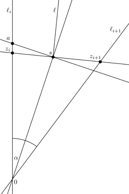 Figure 4
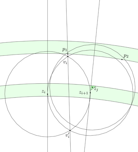 Figure 5
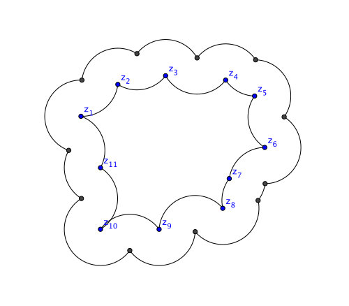 Figure 6
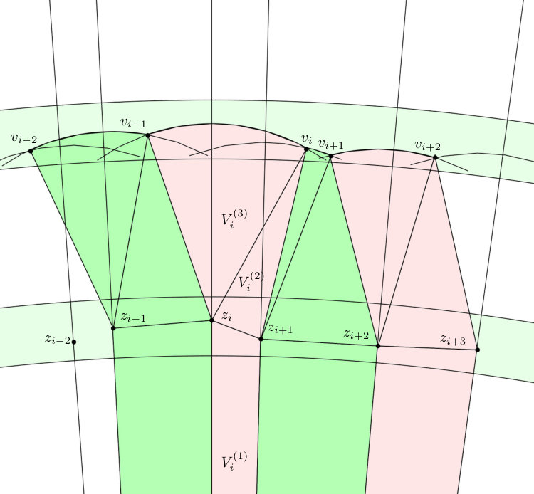 Figure 7
 Figure 8
 Figure 9
Peer Reviews
No public reviews on file for this paper yet. If you reviewed it on a platform where reviews are public (OpenReview, ICLR, NeurIPS, ICML), you can paste yours below so the community can read it here.
Videos
No videos yet. Explain this paper in a talk, walkthrough, or lecture? Add one.
Taxonomy
TopicsStochastic processes and statistical mechanics · Theoretical and Computational Physics · Complex Systems and Time Series Analysis
The Widom-Rowlinson model:
Mesoscopic fluctuations for the critical droplet
Frank den Hollander 111Mathematical Institute, Leiden University, P.O. Box 9512, 2300 RA Leiden, The Netherlands,
Sabine Jansen 222 Mathematisches Institut, Ludwig-Maximilians-Universität, Theresienstrasse 39, 80333 München, Germany,
Roman Kotecký 333Mathematics Institute, University of Warwick, Coventry CV4 7AL, United Kingdom and Center for Theoretical Study, Charles University, Prague, Czech Republic
[email protected] 44footnotemark: 4
Elena Pulvirenti 555Institut für Angewandte Mathematik, Rheinische Friedrich-Wilhelms-Universität, Endenicher Allee 60, 53115 Bonn, Germany
Abstract
We study the critical droplet for a close-to-equilibrium Widom-Rowlinson model of interacting particles in the two-dimensional continuum at low temperature. The critical droplet is the set of macroscopic states that correspond to saddle points for the passage from a low-density vapour to a high-density liquid. We first show that the critical droplet is close to a disc of a certain deterministic radius. After that we analyse the mesoscopic fluctuations of the surface of the critical droplet. These are built on microscopic fluctuations of the particles in the boundary layer, and provide a rigorous foundation for what in physics literature is known as capillary waves.
Our results represent the first detailed analysis of the surface fluctuations down to mesoscopic and microscopic precision. As such they constitute a fundamental step in the study of phase separation in continuum interacting particle systems from the perspective of stochastic geometry. At the same time, they serve as a basis for the study of a non-equilibrium version of the Widom-Rowlinson model, to be analysed elsewhere, where they lead to a correction term in the Arrhenius formula for the average vapour-liquid crossover time.
AMS 2010 subject classifications. 60J45, 60J60, 60K35; 82C21, 82C22, 82C27.
Key words and phrases. Critical droplet, surface fluctuations, large deviations, moderate deviations, isoperimetric inequalities.
Acknowledgment. FdH was supported by NWO Gravitation Grant 024.002.003-NETWORKS, FdH and EP by ERC Advanced Grant 267356-VARIS, and RK by GAČR Grant 16-15238S. EP was supported by the German Research Foundation in the Collaborative Research Centre 1060 “The Mathematics of Emergent Effects”. The authors acknowledge support by The Leverhulme Trust through International Network Grant Laplacians, Random Walks, Bose Gas, Quantum Spin Systems. SJ thanks Christoph Thäle for fruitful discussions.
Contents
-
2.1 Large deviation principles and isoperimetric inequalities
-
3 Proof of large deviation principles and isoperimetric inequalities
-
3.2 Minimisers of the shape rate function and their stability
-
5 Stochastic geometry: approximation of geometric functionals
-
6 Stochastic geometry: representation of probabilities as surface integrals
-
8 Asymptotics of surface integrals: proof of moderate deviations
1 Introduction, background and motivation
Section 1.1 introduces the equilibrium Widom-Rowlinson model. Section 1.2 states a key target in this model, namely, a detailed description of the fluctuations of the so-called critical droplet, i.e., the saddle point in the set of droplets with minimal free energy connecting the vapour state and the liquid state. In [21] we define and analyse a dynamic version of the Widom-Rownlinson model, for which this critical droplet appears as the gate for the metastable transition from the vapour state to the liquid state. Understanding the fluctuations of the critical droplet is crucial for the computation of the metastable crossover time in the dynamic model. The main goal of the present paper is a proof of the key target subject to three conditions, whose proofs are given in [22]. A weaker version of the key target is proved without the three conditions, in order to make the present paper self-contained. Section 1.3 contains an outline of the remainder of the paper.
1.1 The Widom-Rowlinson model
The Widom-Rowlinson model is an interacting particle system in where the particles are discs with an attractive interaction. It was introduced in Widom and Rowlinson [38] to model liquid-vapour phase transitions, and is one of the rare models in the continuum for which a phase transition has been established rigorously. In the present paper we place the particles on a finite torus in .
Fix and let be the torus of side-length . We can identify with the set after we redefine the distance by
[TABLE]
The set of finite particle configurations in is
[TABLE]
where denotes the cardinality of , i.e., particles are viewed as non-coinciding points that are indistinguishable. The halo of a configuration is defined as (see Fig. 1)
[TABLE]
where is the closed disc of radius centred at . (The reason why we choose radius instead of radius is explained in [21]: the one-species model arises as the projection of a two-species model.) The energy of a configuration is defined as
[TABLE]
where and . The energy vanishes when the discs do not overlap, and reaches its minimal value when the discs coincide. Since , the interaction is attractive and stable (Ruelle [29, Section 3.2]).
We define the grand-canonical Hamiltonian in with chemical potential as
[TABLE]
The grand-canonical Gibbs measure is the probability measure on defined by
[TABLE]
where is the inverse temperature, is the law of the homogeneous Poisson point process on with intensity , and is the normalisation
[TABLE]
Write to denote the chemical activity. In the thermodynamic limit, i.e., when , a phase transition occurs at with (see Fig. 2)
[TABLE]
(Ruelle [30], Chayes, Chayes and Kotecký [8]). No closed form expression is known for the critical inverse temperature . We place ourselves in the metastable regime
[TABLE]
In other words, we choose to lie in the liquid phase region, above the phase coexistence line in Fig. 2 representing the phase transition in the thermodynamic limit, and we let and in such a way that we keep close to the phase coexistence line by a fixed factor . For this choice the Gibbs measure in (1.6) becomes
[TABLE]
so that large particle numbers are favoured while large halos are disfavoured.
Let be the homogeneous Poisson point process on with intensity . If denotes the law of , then is absolutely continuous with respect to with Radon-Nikodym derivative
[TABLE]
1.2 A key target: the critical droplet
For , abbreviate (see Fig. 3),
[TABLE]
Throughout the paper, and are fixed (recall that is the linear size of the torus ). Define
[TABLE]
where is a constant that will be identified below and that does not depend on .
Fix , abbreviate , and define
[TABLE]
As shown in [21], appears as the leading order term in a computation of the Dirichlet form associated with a dynamic version of the Widom-Rowlinson model. In this dynamic version, the special role of the critical disc becomes apparent through the fact that the set forms the gate for the metastable transition from the gas phase (‘ empty’) to the liquid phase (‘ full’) in the metastable regime (1.9). The main ingredient in [21] is the following sharp asymptotics.
TARGET: For large enough and ,
[TABLE]
The above target is a statement about a restricted equilibrium: it provides a sharp estimates for the probability that the halo has a volume that lies inside an interval of width around the volume of the critical disc . By writing
[TABLE]
we see that we may think of as (a leading order approximation of) the free energy of the critical droplet, consisting of the bulk free energy and the surface tension, and of as (a leading order approximation of) the entropy associated with the fluctuations of the surface of the critical droplet, which plays the role of a correction term to the free energy. We will see that there are order discs inside the critical droplet and order discs touching its boundary (see Fig. 4). We remark that is to be viewed as a dimensionless quantity, i.e., the inverse temperature divided by some unit of energy. Otherwise, its fractional powers would not make sense.
The goal of the present paper is to provide a proof of (1.15), subject to three conditions that are settled in [22]. To make the present paper self-contained, we also prove a rough asymptotics that does not require these conditions, but still provides the correct order of magnitude for the entropy term, with bounds on the constant in (1.13). Along the way we will see that
[TABLE]
Since does not depend on , we may view (1.15) as a weak large deviation principle for the random variable under the Gibbs measure in (1.10). The rate is and the rate function is degenerate, being equal to the constant . This degeneracy reflects the fact that the radius of the critical droplet is close to , for which .
1.3 Outline
In Section 2 we present our main theorems: a large deviation principle for the halo shape and the halo volume, and weak moderate deviations for the halo volume close to the critical droplet. These theorems are the main input for the analysis of the dynamic Widom-Rowlinson model in [21]. Section 3 proves the two large deviation principles, as well as certain isoperimetric inequalities that play a crucial role throughout the paper. In Section 4 we provide the heuristics behind the proof of the main theorems, which is carried out in Sections 5–8. Section 5 focusses on approximations of certain key geometric functionals, which are crucial for the analysis of the moderate deviations. Section 6 represents moderate deviation probabilities in terms of geometric surface integrals and introduces auxiliary random processes that are needed for the description of the fluctuations of the surface of the critical droplet. Section 7 contains various preparations involving exponential functionals of the auxiliary random variables. Section 8 uses these preparations, in combination with the geometric properties derived in Sections 5–7, to prove the moderate deviations for the halo volume close to the critical droplet.
The results in Sections 3–8 lead to a description of the mesoscopic fluctuations of the surface of the critical droplet in terms of a certain constrained Brownian bridge and quantifies the cost of moderate deviations for the surface free energy of droplets. The proof relies on three conditions involving the microscopic fluctuations of the surface of the critical droplet, whose proofs are given [22]. To make the present paper self-contained, we also prove a rough moderate deviation estimate that does not need the three conditions.
2 Main theorems
This section formulates and discusses our main theorems. In Section 2.1 we state large deviation principles for the halo shape (Theorem 2.1) and the halo volume (Theorem 2.3), and show that the corresponding rate functions are linked via an isoperimetric inequality (Theorem 2.2). In Section 2.2 we formulate a conjecture (Conjecture 2.4) about moderate deviations for the halo volume, and state a sharp asymptotics that settles a version of this conjecture for volumes that are close to the volume of the critical droplet (Theorem 2.5). This sharp asymptotics settles the target formulated in Section 1.2, subject to three conditions (Conditions (C1)–(C3) below), whose proof is given in [22]. In order to make our paper self-contained, we also prove a rougher asymptotics (Theorem 2.6), which does not require the conditions and still provides the correct order of the correction term, with explicit bounds on the constant. In Section 2.3 we place our results in a broader context and explain why they open up a new window in the area of stochastic geometry for interacting particle systems.
For background on large deviation theory, see e.g. Dembo and Zeitouni [11] or den Hollander [20].
2.1 Large deviation principles and isoperimetric inequalities
Admissible sets.
Let be the family of non-empty closed (and hence compact) subsets of the torus . We equip with the Hausdorff metric
[TABLE]
where . This turns into a compact metric space (Matheron [27, Propositions 12.2.1, 1.4.1, 1.4.4], Schneider and Weil [31, Theorems 12.2.1, 12.3.3]). Let be the collection of all sets that are -)admissible, i.e.,
[TABLE]
where is the halo of . In Section 3.1 we will see that there is a unique maximal such that , which we denote by and which equals .
Obviously, not every closed set is admissible. For example, when we form -halos we round off corners, and so a shape with sharp corners cannot be in . Also note that whenever is admissible: necessarily contains at least one disc with . In the following, we typically omit the subscript referring to the torus .
Large deviation principles.
Define
[TABLE]
and
[TABLE]
We view the halo as a random variable with values in the space , topologized with the Hausdorff distance. Note that because .
Theorem 2.1** (Large deviation principle for the halo shape).**
The family of probability measures satisfies the LDP on with speed and with good rate function .
Informally, Theorem 2.1 says that
[TABLE]
The contraction principle suggests a large deviation principle for the halo volume. To formulate this, we first state a minimisation problem. The condition below ensures that that the effect of the periodic boundary conditions on the torus is not felt.
Theorem 2.2** (Minimisers of rate function for halo volume).**
**
- (1)
For every ,
[TABLE]
and the minimisers are the discs of radius .
- (2)
The minimisers are stable in the following sense: There exists an such that if and satisfies
[TABLE]
then is connected with connected complement (simply connected as a subset of ), and
[TABLE]
where denotes the Hausdorff distance.
Theorem 2.2 is a powerful tool because it shows that the near-minimers of the halo rate function are close to a disc and have no holes inside. In particular, it tells us that
[TABLE]
and allows us to describe the large deviations of the halo volume.
Theorem 2.3** (Large deviation principle for the halo volume).**
The family of probability measures satisfies the LDP on with speed and with good rate function given by
[TABLE]
Informally, Theorem 2.3 says that
[TABLE]
For every , we have
[TABLE]
2.2 Near the critical droplet: moderate deviations
Fluctuations of the halo volume.
The function is maximal at
[TABLE]
We assume that . In the dynamic Widom-Rowlinson model that we introduce and analyse in [21], plays the role of the radius of the critical droplet for the metastable crossover from an empty torus to a full torus in the limit as . We therefore zoom in on a neighborhood of the critical droplet. The large deviation principle yields the statement
[TABLE]
for fixed. We would like to take , for which we need a stronger property.
Conjecture 2.4** (Weak moderate deviations for the halo volume).**
There exists a function such that
[TABLE]
Conjecture 2.4 has the flavor of a weak large deviation principle on scale with speed . For we expect the function to be constant. In Theorem 2.5 below we establish a version of this claim, with , the entropy defined in (1.13). In what follows we first state a theorem (Theorem 2.5 below) that relies on three conditions involving an effective interface model whose proof is given in [22]. Afterwards we state a weaker version (Theorem 2.6 below) that provides upper and lower bounds, whose proof is fully completed in the present paper. To state these theorems we need some additional notation.
Notation.
Let be the halo of some configuration . The boundary of consists of a union of circular arcs that are disjoint except for their endpoints. We call the centres of these circles the boundary points of and we say that is a connected outer contour if there exists a halo with a simply connected -interior having exactly these boundary points (see Fig. 5). Let
[TABLE]
Later on we parametrize the boundary points of an approximately disc-shaped droplet in polar coordinates. We will see that, roughly, we may think of the angular coordinates as the points of an angular point process, and of the radii as the values of a Gaussian process evaluated at those random angles. To make this picture more precise, we need to introduce auxiliary processes.
Let be standard Brownian motion starting in [math], and let
[TABLE]
be standard Brownian bridge on . Consider the process
[TABLE]
called the mean-centred Brownian bridge (Deheuvels [10]). Set
[TABLE]
Let
[TABLE]
Thus, is a Poisson random variable with parameter . We assume that and are defined on a common probability space and they are independent. Conditional on the event , we may write with , and define
[TABLE]
Note that , , and . For , set
[TABLE]
with
[TABLE]
Later we will see that the natural reference measure for the angles is not the Poisson process but a periodic version of a renewal process, which is conveniently constructed by tilting the distribution of the Poisson process . The precise expression for the exponential tilt will be derived later. Set
[TABLE]
and consider the tilted probability measure on defined by
[TABLE]
Finally let be the unique solution to the equation
[TABLE]
The change of variables together with yields
[TABLE]
and so . In the sequel we use the notation , .
Conditions.
Our main theorem builds on three conditions whose validity is proven in [22]:
- (C1)
The limit
[TABLE]
exists and is of the form
[TABLE]
for some that does not depend on . 2. (C2)
The change from to does not affect (C1) when is not too large:
[TABLE] 3. (C3)
Let
[TABLE]
and
[TABLE]
Then, for sufficiently small,
[TABLE]
uniformly in .
Condition (C1) comes from the fact that for each of the boundary points there is a constraint in terms of the two neighbouring boundary points that must be satisfied in order for the corresponding 2-disc to touch the boundary of the critical droplet. The constant is related to the free energy of an effective interface model. Condition (C2) says that the constraint imposed by condition (C1) is not affected by small dilations of the critical droplet, and implies that the free energy of the effective interface model is Lipschitz under small perturbations. Condition (C3) says that the first Fourier coefficient of the surface of the critical droplet is small. The term represents an energetic and entropic reward for the droplet boundary to fluctuate away from . We require that this reward – which may be thought of as a background potential in the effective interface model – does not affect the microscopic free energy of the droplet.
Main theorem: sharp asymptotics.
We are now ready to formulate our main theorem.
Theorem 2.5** (Moderate deviations).**
Suppose that conditions (C1)–(C3) hold. Then, for large enough and ,
[TABLE]
where
[TABLE]
In view of (1.14) and (1.17), Theorem 2.5 settles the target in (1.15) subject to conditions (C1)–(C3).
Rough asymptotics.
Without conditions (C1)–(C3) we can still prove the following rougher asymptotics, which makes our paper self-contained.
Theorem 2.6** (Moderate deviation bounds).**
For large enough,
[TABLE]
with some constant (that may depend on ).
Theorem 2.5 provides a full description of the fluctuations of the surface of the critical droplet in the Widom-Rowlinson model in the metastable regime (1.9). It makes fully precise and rigorous the heuristic arguments for capillary waves that are put forward in Stillinger and Weeks [37]. In the proof of Theorem 2.5 in Sections 5–8 we will see that the boundary points are given by (2.23), with the mean-centred Brownian bridge, the Poisson point process on with intensity tilted via the probability measure in (2.25), and (which is negligible). We will also see that the effect of centring of the droplet is that the discrete Fourier coefficients defined in (2.31) are asymptotically vanishing.
2.3 Context
In this section we place our main theorems in the broader context of stochastic geometry and continuum statistical physics. For general overviews we refer the reader to Chiu, Stoyan, Kendall and Mecke [9], respectively, Georgii, Häggström and Maes [17].
Large and moderate deviations for confined point processes.
There is a rich literature on limit laws for high-intensity point processes and extremal points, and also on the high-intensity Widom-Rowlinson model. Let us explain why Theorem 2.5 is considerably more involved than the theorems encountered in that literature. We first review two papers in the context of stochastic geometry that are close in spirit to our results and discuss the differences. The results from the point process literature are valid in higher dimensions as well, but for simplicity we present the summary for only.
Consider a disc of fixed radius and a homogeneous Poisson point process with intensity in . The set is called the vacant set, the volume is called the defect volume. A point is extremal when . Write for the indicator that is extremal in . (The problem has been also studied for general compact sets instead of , in which case the points are called -maximal.) The following results are available in the limit as :
(I) Schreiber [33] focusses on a Boolean model that is a variation on the Widom-Rowlinson model, in which to each point of the Poisson point process a random closed set called grain is attached. Grains are deterministic compact convex smooth sets satisfying certain conditions, namely, they are contained in , are twice differentiable on the boundary, and are parametrized by the point closest to the boundary of . The following results are proved in [33]:
(i) A law of large numbers for the defect volume:
[TABLE]
(ii) A moderate deviation estimate: if is the expected defect volume, then for all and some ,
[TABLE]
The limit exists. An LDP is proved for a point process whose law is a Gibbsian modification of a Poisson point process with a hard-core Hamiltonian, which describes the one-color process in the two-color Widom-Rowlinson model. This result is close to our LDP, the main difference being that the minimization is much easier than in our model.
(II) Schreiber [34] considers a homogeneous Poisson point process with intensity restricted to (which by abuse of notation we again call ) and proves the following: satisfies the full LDP on with rate and with good rate function , the so-called Caccioppoli perimeter. However, this is proved in a specific limit for and jointly, namely,
[TABLE]
(i.e., the large-volume limit and the high-intensity limit are taken simultaneously), while in our setting the volume of the system and the radius of the discs are kept fixed. Furthermore, the parameters of the model are taken to be on the coexistence line. In our case this would amount to taking the limit instead of fixing arbitrarily.
In Section 3 we give a full description of large deviations for arbitrary droplets, and in Sections 5–8 of moderate deviations for near-critical droplets. The fluctuations that we consider are two-sided, i.e., the droplets are not confined to an ambient disk but rather live on a torus.
Interface literature.
Another popular concept in stochastic geometry is that of random convex polytope and its relation with the paraboloid growth process (see Schreiber and Yukich [35], Calka, Schreiber and Yukich [7]). The former is the convex hull of (with a smooth convex set in ), the latter is a growth model for interfaces that is studied because it provides information on the asymptotic behaviour as of geometric functionals of random polytopes, in particular, on the distribution of -maximal points. While we marginally touch on these concepts in the present paper, they play an important role in [22], where we discuss the microscopic fluctuations of the surface of the critical droplet. There we prove that, upon rescaling of the random variables describing the boundary of the critical droplet, the effective microscopic model is given by a modification of the paraboloid hull process, which is connected to the paraboloid growth process. In [22], the conditions (C1)–(C3) in Theorem 2.5 are formulated in the context of paraboloid hull processes, and are proven there.
The literature on stochastic interfaces is large, especially for phase boundaries separating two phases. In statistical mechanics interface analyses have been successfully carried out for discrete systems, such as the Ising model. Higuchi, Murai and Wang [19] adapted to the two-dimensional Widom-Rowlinson model what was done in Higuchi [18] for the two-dimensional Ising model. As for the Ising model, the interface is well approximated by that of the so-called Solid-on-Solid model. The results in [19] concerns limiting properties of the continuous random processes that model the fluctuations of the interface in the direction orthogonal to the line connecting the two end points of the phase boundary. Diffusive scaling of the interface is shown, with Brownian bridge appearing as the limit. However, the results in [19] are again only for parameters on the coexistence line, which in our case amounts to taking the limit .
Further variations on the Widom-Rowlinson model.
Several further variations on the Widom-Rowlinson model have been considered in the literature. One is the so-called area-interaction point process considered in Baddeley and van Lieshout [4], where the probability density of a point configuration depends on the area of through a parameter . When , the Widom-Rowlinson model is recovered. Another is the so-called quermass-interaction processes introduced in Kendall, van Lieshout and Baddeley [25], where a Boolean model interacting via a linear combination of Minkowski functionals generalizes the above area-interaction. In both these papers the problem of well-posedness of the processes are addressed via a proof of integrability and stability in the sense of Ruelle [29], but no result in terms of large deviations are obtained.
Another generalization regards the multi-color Widom-Rowlinson model (see Chayes, Chayes and Kotecký [8]): colors are considered and random radii , , are attached to any color. In Dereudre and Houdebert [12] the case with non-integrable random radii is studied, and a different type of phase transition is proved.
3 Proof of large deviation principles and isoperimetric inequalities
In this section we prove Theorems 2.1–2.3. Section 3.1 takes a closer look at the properties of admissible sets (Lemmas 3.1–3.2). Section 3.2 gives the proof of Theorem 2.2. The proof requires two isoperimetric inequalities (Lemmas 3.3–3.4), which are analogues of the classical isoperimetric and Bonnesen inequalities, and imply that the minimisers of in (2.4) are discs and that the difference of with its minimum can be quantified in terms of the Hausdorff distance to these discs. Section 3.3 proves the large deviation principle for the centres of the 2-discs in the Widom-Rowlinson model (Proposition 3.5), and uses this to prove Theorems 2.1 and 2.3.
3.1 Properties of admissible sets
Write
[TABLE]
for the -halo of (Minkowski addition) and
[TABLE]
for the 2-interior of (Minkowski subtraction). In integral geometry, the sets and are called the dilation and the erosion of , respectively. Note that the erosion and subsequent dilation of a set is contained in , i.e.,
[TABLE]
(Matheron [27, Section 1.5]). See Lemma 3.1(1) below.
Note that is not necessarily equal to . We use to denote the collection of all sets for which equality holds and call them (-)admissible (open with respect to in the terminology of integral geometry), i.e.,
[TABLE]
In the following, we typically omit the subscript referring to the torus , by writing , . There is another useful characterisation of admissible sets: if and only if it is the 2-halo of some , (see Lemma 3.1(2) below). Obviously, not every closed set is admissible. For example, when we form 2-halos we round off corners, and so a shape with sharp corners cannot be in . Also note that whenever is admissible: necessarily contains at least one disc with .
In this section we summarise some known properties of admissible sets in a setting that will be needed later. The proofs of these properties rely on various sources. Below we only quote appropriate references, and when instructive we supply a short proof.
A key property is that for any set such that is connected and is simply connected, the set is of reach at least 2. Recall that the reach of a set is
[TABLE]
Lemma 3.1**.**
- (1)
If , then . 2. (2)
* if and only if is the -halo of some , i.e.,*
[TABLE] 3. (3)
Both and are continuous with respect to the Hausdorff metric. 4. (4)
If and is connected, then also is connected. 5. (5)
If is convex, then and are convex and . If are convex and , then also . 6. (6)
The set is the closure in of the set , where consists of all of the form with finite. 7. (7)
If , then , provided the following condition is satisfied:
[TABLE] 8. (8)
For any such that , the boundary is -rectifiable. If , then the boundary is Lipschitz.
Proof.
We indicate the proper references to the literature. Part (7) is delicate.
(1) (Matheron [27, Chapter 1.5]) Note that is equivalent to , which is equivalent to the existence of a . Hence, since and since . In [27], sets such that are called open w.r.t. (rather than admissible).
(2) (Matheron [27, Chapter 1.5]). For any , we have with . On the other hand, if , then since and hence . The inclusion , which amounts to , was proven in 1.
(3) For the first claim, see Matheron [27, Proposition 1.5.1] Schneider and Weil [31, Theorem 12.3.5], for the second claim, see Kampf [24, Lemma 9].
(4) See Matheron [27, Chapter 1.5].
(5) See Matheron [27, Proposition 1.5.3]. In [27] , sets such that are called closed w.r.t. .
(6) This follows from the fact that finite sets are dense in in combination with the first claim in (3).
(7) Use Federer [13, Theorem 5.9], which assures that the is conserved under taking limits of sets with respect to the Hausdorff metric. It therefore suffices to consider with , where the finite set is sufficiently dense so that condition (C) is satisfied for .
We will prove that, for such , . First, observe that the boundaries and are unions of circular arcs (of radius 2). Given that satisfies condition (C), the set splits into connected components, each bordered by two Jordan curves: one connected component of the boundary and one connected component of the boundary . For each component of , we label the centres of the arc circles in such a way that two consecutive arcs belong to two consecutive centres, with periodic boundary condition. The associated component of is a union of circular arcs passing through the centres. The centre of the arc circle connecting two consecutive centres is the point on the boundary in the intersection of the arcs with these centres.
Let us assume that . Then there exist a point and two distinct points in a connected component of the boundary such that . (To belong to two distinct components of contradicts assumption (C).) Given that , the interior of the disc does not contain any point from , i.e., . In addition, there are at most finitely many points of in , all of which belong to .
The admissibility of means that every disc of radius 2 with a centre on is fully contained in . We will draw a contradiction with this statement from the fact that a Jordan curve avoiding and containing two distinct points on its boundary necessarily indents too sharply to be consistent with admissibility of and condition (C). To show the contradiction, consider a line through the point that separates the points and into opposite half planes determined by . Without loss of generality, we may assume that the points do not belong to . As a result, both and contain points not in or, since , there exist points and such that . Now, and cannot contain any point from , and hence the Jordan curve must avoid with , which yields the contradiction with condition (C).
Indeed, if is the outer boundary of the set with a single outer component of , then in contradiction with condition (C) this component contains two components of , since the points and belong to different components of . Otherwise, the Jordan curve is the inner boundary of the set and surrounds the set . However, the region encircled by contains two different components of , one containing and the other containing .
(8) For the first claim, see Ambrosio, Colesanti and Villa [2, Proposition 3]. For the second claim, it suffices to note that for the boundary is a finite union of arcs. ∎
We will also need the Steiner formula for sets of positive reach (Federer [13]).
Lemma 3.2**.**
Let be an admissible set with of reach at least . Then
[TABLE]
where is the outer Minkowski content of and is the Euler-Poincaré characteristic of (= the number of connected components minus the number of holes). If the boundary is Lipschitz, then , where is the -dimensional Hausdorff measure.
Proof.
Reformulating the Steiner formula for sets of positive reach as defined by Federer [13, Theorem 5.5, Theorem 5.19], we get, for and ,
[TABLE]
for any and by continuity also for . For continuity of the left-hand side, see Sz.-Nagy [28]. The last claim is the same as Ambrosio, Colesanti and Villa [2, Corollary 1]. ∎
3.2 Minimisers of the shape rate function and their stability
In this section we prove Theorem 2.2.
(1) The proof relies on the Brunn-Minkowski inequality and on Lemma 3.3 below, which provides three reformulations of the isoperimetric inequality in (2.6).
Lemma 3.3**.**
Let . If and , then the following three statements are equivalent:
- (a)
.
- (b)
.
- (c)
.
Moreover, equality holds in (a), (b), and (c) simultaneously, or in none.
Proof.
The equivalence of (b) and (c) is an immediate consequence of the fact that . For the equivalence of (a) and (b), we observe that and therefore, with , (a) is equivalent to
[TABLE]
We add to both sides and take the square to find that (a) is equivalent to (b). ∎
Proof of Theorem 2.2.
Armed with Lemma 3.3, we employ the Brunn-Minkowski inequality
[TABLE]
which is valid for any non-empty measurable , and (see Lusternik [26] and Federer [14, 3.2.41]). Indeed, (3.10) with implies
[TABLE]
and yields inequality (c) with and , and thus also (2.6) by (a). Equality in (3.11) occurs only if is a disc or a point (see Burago and Zalgaller [3, Section 8.2.1]).
(2) We first prove that if is close to a minimiser, then necessarily is connected and simply connected.
Lemma 3.4**.**
There exist a function satisfying such that if satisfies (2.7) with , then
[TABLE]
for sufficiently small , and is connected and simply connected.
Proof.
We use the claim about the stability of the Brunn-Minkowski inequality, first proven in qualitatively by Christ [6] and then quantitatively by Figalli and Jerrison [16]. Actually, for our purposes the qualitative version [6] suffices, since we are only using it as a springboard for more accurate bounds to be considered later.
Adapted to our setting, the claim is that there exist positive function with , such that if
[TABLE]
with sufficiently small , then there exist a compact convex set such that
[TABLE]
In the same vein, a (properly scaled and shifted) disc satisfies
[TABLE]
To verify the assumption in (3.13), we rewrite (2.7) as
[TABLE]
and use an equivalent formulation of (3.13), namely,
[TABLE]
Indeed, (3.16) with implies that the LHS of (3.17) is bounded by which, with the choice is bounded by the right-hand side of (3.17) and thus also (3.13).
Note that, in view of the convexity of , the condition in (3.15) implies that . Indeed, suppose without loss of generality that the centre of the disc is at the origin and write for its radius, so that . If , then contains the union of and the wedge bordered by and the tangents through to . The volume of this wedge is . Asymptotically, for small , this equals and exceeds once . Thus, and
[TABLE]
For an admissible , we can significantly strengthen the second claim in (3.14). We can argue that with . Indeed, if , then , while (see [21, Eq. (D.8)], in contradiction with the second inequality in (3.14). Combining the present claim with (3.18), we get
[TABLE]
Given that , this implies
[TABLE]
yielding, for sufficiently small , the statement in (3.12) with
[TABLE]
Using that
[TABLE]
we will prove connectedness and simple connectedness of the set by showing that every segment in the direction of any unit vector , intersects the set in a closed interval: with . If the contrary were true, then there would be a direction and two points , such that and . The fact that implies that , while implies that , and hence, in view of the preceding inclusion, . However, this cannot happen when . Nevertheless, this is exactly what happens when . Indeed, once , where is the line through orthogonal to . For we have
[TABLE]
when , which is equivalent with . ∎
To finish the proof of Theorem 2.2, we use that is connected and simply connected once (2.7) is satisfied and . For the latter, similarly as in the proof of Lemma 3.1 7, we may assume that . For fixed we choose such that for any . Using now that according to Lemma 3.1(7), we will rely on the Bonnesen inequality, which is more precise than the provisional claim in (3.12) with the bound whose dependence on is not explicitly specified. For connected and simply connected , its boundary is a Jordan curve and according to the Bonnesen inequality the difference of the radii and of the outer and the inner circle of the curve can be bounded in terms of the isoperimetric defect :
[TABLE]
Assuming that , we can write
[TABLE]
with the help of the Steiner formula (Lemma 3.2) and reformulate the isoperimetric defect as
[TABLE]
If the left-hand side of (3.25) is , then the right-hand side of (3.26) is bounded from above by
[TABLE]
It follows from (3.24) that
[TABLE]
Since , we get the claim in (2.8). ∎
3.3 Large deviation principle for Widom-Rowlinson
In this section we prove Theorems 2.1 and 2.3.
Remember the Gibbs measure at inverse temperature and activity . This is a probability measure on the space of particle configurations, which we may view as a subset of equipped with the Hausdorff topology. By a slight abuse of notation, we identify on with the measure on supported on . Theorem 2.1 builds on the large deviation principle for the Gibbs measure itself, i.e., the large deviation principle for the set of particle locations.
The LDP for is summarised in the following proposition (recall that a rate function is called good when it is lower semi-continuous and has compact level sets). This proposition is in the spirit of Schreiber [32], [33, Theorem 1]. The latter is stated in a slightly different setting, but the main ideas of the proof carry over.
Proposition 3.5** (Large deviation principle for Widom-Rowlinson).**
The family of probability measures on , supported on , satisfies the LDP with rate and good rate function given by
[TABLE]
Proof.
Let be the homogeneous Poisson point process on with intensity . We may view as a random variable on a probability space taking values in . Since , , it follows that the family satisfies the large deviation principle with rate and good rate function , . Note that is upper semi-continuous (Schneider and Weil [31, Theorem 12.3.5]), but not continuous: sets of positive measure can be approximated by finite sets, which have measure zero. It follows that is lower semi-continuous, but not continuous. Nevertheless, the map is continuous with respect to the Hausdorff metric (see Lemma 3.1(3)). Therefore, since
[TABLE]
the claim follows from the LDP for the Poisson point process and Varadhan’s lemma. ∎
With the help of Proposition 3.5, the proof of Theorems 2.1 and 2.3 becomes straightforward via the contraction principle.
Proof of Theorem 2.1.
As mentioned above, the map defined by is continuous with respect to the Hausdorff metric. Proposition 3.5 and the contraction principle therefore imply that the LDP for the law of under holds with rate and good rate function given by
[TABLE]
We show that . Indeed, if , then and yielding . On the other hand, taking with in view of admissibility of , we get . ∎
Proof of Theorem 2.3.
Theorem 2.3 follows from Proposition 3.5, the continuity of the map , and the contraction principle. The rate function is given by
[TABLE]
In the difference of the two infima, the first infimum (when with ) is equal to by Theorem 2.2. For the second infimum, we note that
[TABLE]
with equality for . ∎
4 Heuristics for moderate deviations
In this section we provide the main ideas behind the proof of Theorems 2.5–2.6 in Sections 5–8. Guidance is needed because the proof is long and intricate. In Section 4.1 we explain how the moderate deviation probability for the halo volume can be expressed in terms of a certain surface integral. In Section 4.2 we explain how the weight in this surface integral can be approximated in terms of the polar coordinates of the boundary points. In Section 4.3 we provide a quick guess of what the orders of magnitude of the angles and the radii of the boundary points are as . In Section 4.4 we introduce auxiliary random processes that allow us to transform the surface integral into an expectation of a certain exponential functional, capturing the global (= mesoscopic) scaling of the boundary of the critical droplet. In Section 4.5 we perform a further change of variable to rewrite the expectation in terms of an effective interface model, capturing the local (= microscopic) scaling of the boundary of the critical droplet.
4.1 Reduction to a surface integral
The starting point for the proof of Theorem 2.5 is the following. Because of the large deviation principles in Theorems 2.1 and 2.3 and the quantitative isoperimetric inequality 2.2, the dominant contribution to the event should come from approximately disc-shaped halos (“droplets”). Consider the event
[TABLE]
that is close to a disc , without any holes. Because of the translation invariance of the model, we may focus on .
For , the boundary of the droplet is a union of circle arcs centreed at points , called boundary points. Each boundary point is extremal in the sense that . We call a collection of points a connected outer contour if there exists a halo with a simply connected -interior having exactly these boundary points. The halo , if it exists, is unique, and we denote it by . The set of connected outer contours is denoted by .
For , both and are uniquely determined by the boundary points, since and . Therefore it makes sense to compute probabilities by conditioning on the boundary points. Abbreviate
[TABLE]
We will see that the following is true: for some constant and for all measurable sets , as ,
[TABLE]
where is the collection of connected outer contours for which , and is the rate function defined in (2.10). In view of this geometric constraint, the only contributions to the right-hand side of (4.3) are from connected outer contours that lie in an annulus: , . Hence we may think of (4.3) as a surface integral.
4.2 Approximation of the surface term
In view of (4.3), our next task is to evaluate . Let us choose polar coordinates for the boundary points and write
[TABLE]
Upon relabelling the centres, we may without loss of generality assume that . We set and , and define angular increments
[TABLE]
Note that and . The volume of the shape with boundary points admits an expansion
[TABLE]
Also,
[TABLE]
The previous formulas are valid for general radius . Next we specialize to . With
[TABLE]
and using that , we get
[TABLE]
with
[TABLE]
4.3 Orders of magnitude
Neglecting higher order terms in in (4.9), we see that the weight involves several terms. The factor suggests that the typical angular increment is of order , and the typical number of boundary points therefore is of order . The factor
[TABLE]
suggests that is approximately normal with variance proportional to . Hence, we expect that the radial increment is typically of order . Combining these observations, we may expect that
[TABLE]
which explains the exponent in Theorem 2.5. Furthermore, it will be natural to think of as
[TABLE]
with some unknown mean value, and the mean-centred Brownian bridge from (2.18). The consistency with the guessed order of magnitude of the radial increment is guaranteed by the fact that and the observation that . Finally, we note that
[TABLE]
which should not contribute at the scale we are interested in (unless is large). Nevertheless, we will need to treat this term carefully because, for the mean-centred Brownian bridge we have
[TABLE]
and extra arguments will be needed to cure this divergence.
For later purpose, let us also have a closer look at the volume constraint . If we substitute the expression (4.6) for and neglect higher order terms, then the volume constraint becomes
[TABLE]
Making a few leaps of faith, we may approximate
[TABLE]
using that for the mean-centred Brownian bridge. From the considerations above we should expect the sum overall to be of order . Hence should also be of order , i.e., . Later we will only prove that , but this will turn out to be enough for our purpose.
4.4 Global scaling: auxiliary random processes
If we substitute the approximation (4.9) for into the surface integral in (4.3) and drop error terms and indicators, we are naturally led to the investigation of expressions of the type
[TABLE]
where is some non-negative test function, and we recall (4.4) and (4.8) (by convention the summand with equals ). The Gaussian term (see also (4.11)) is conveniently expressed with the heat kernel
[TABLE]
and we have
[TABLE]
Let us approximate , drop the term , and change variables as . Then the integral in (4.18) becomes
[TABLE]
With the help of
[TABLE]
and , the expression (4.21) is rewritten as
[TABLE]
This expression motivates the auxiliary processes and the expressions and introduced before Theorem 2.5. Moreover, and only enter in the combination (except possibly in the test function ), which explains the scaling of the surface corrections in Theorem 2.5.
The picture that emerges of the droplet boundary is that its deviation from should be of the order of , and that the boundary points are obtained by selecting points of a Gaussian curve according to an angular point process. The process has a number of points of order . We may call this picture global since it describes the overall shape of the droplet – the Gaussian process does not see the microscopic details.
4.5 Local scaling: effective interface model
Equation (4.18) suggests one last change of variables, namely, set
[TABLE]
Note that
[TABLE]
Then (4.21) becomes
[TABLE]
or, equivalently,
[TABLE]
Let us finally return to the term that we had dropped from (4.18). By (4.25), we have
[TABLE]
Taking this term into account, we see that (4.27) should be replaced by the more accurate integral
[TABLE]
We may view the exponential, together with an additional indicator for the boundary points, as the Boltzmann weight for an effective interface model, which is studied in detail in [22]. The term plays the role of a background potential.
5 Stochastic geometry: approximation of geometric functionals
This section collects a number of geometric facts that will be needed for the moderate deviations of the halo volume. In Section 5.1 we prove a number of a priori estimates on the radial and the angular coordinates of the boundary points, i.e., the centres of the discs that lie at the boundary of the critical droplet (Lemma 5.1, Proposition 5.2, Definition 5.3 and Corollary 5.4). These estimates play a crucial role for the arguments in Sections 6–8. In Section 5.2 we show that the set of boundary points allows for a local characterisation, in the sense that whether or not a 2-disc touches the boundary of the critical droplet only depends on the centre of the two neighbouring 2-discs (Definition 5.5, Lemma 5.6 and Proposition 5.7). In Section 5.3 we derive an approximation for the volume and the surface of halos that are close to a critical disc, in terms of certain sums involving the radial and the angular coordinates of the boundary points (Proposition 5.8). In Section 5.4 we do the same for the geometric centre of halos that are close to a critical disc (Proposition 5.9 and Corollary 5.10). The a priori estimates in Sections 5.1 allow us to control the approximations derived in Sections 5.3–5.4.
5.1 A priori estimates on boundary points
Theorem 2.2 can be applied to sets of the form , the halo of the configuration . In particular, the condition that the boundary is close to a disc with is a strong restriction on the geometry of the boundary points (recall Fig. 5).
In this section we collect several a priori estimates and constraints that follow from the fact that has a simply connected 2-interior and . Remember the notion of boundary points, connected outer contour , and the polar introduced in Section 4.1 and the polar coordinates and angular increments from (4.4) and (4.5). We write or to denote the ray from the origin passing through the point , and and to denote the -annuli defined as the closures of and , respectively.
First we show that the intersections of the boundary circles in follow the order of the corresponding boundary points:
Lemma 5.1**.**
Fix . If and , then as :
- (a)
* for all .*
- (b)
The distance between any two points such that satisfies
[TABLE]
and the angle between the rays and satisfies
[TABLE]
- (c)
For every there exists a unique such that .
- (d)
The boundary consists of the union of closed arcs of the circles between the points and , , contained in (with ).
Proof.
The proof is based on a number of geometric observations.
(a) This claim is immediate from the fact that and that each is a boundary point with and .
(b) Let . To get the bound in (5.1), we note that the maximal distance between and and the maximal angle consistent with the condition and occur when and , i.e., when the ray is orthogonal to the segment . Assume, without loss of generality, that and with . Then the condition reads
[TABLE]
which, in combination with the equation , yields and implies
[TABLE]
which settles (5.1). For the corresponding angle, we have , and hence , which settles (5.2).
(c) Let and consider the boundary piece . This consists of two arcs, and , both ending in the points and . A necessary condition for both and to be boundary points is that both arcs and intersect the annulus . If, in addition, , then we get a contradiction with the assumption that both and are boundary points. Indeed, consider the line through and (and through ) and the intersection point as shown in Fig. 6.
There exists such that . Otherwise there would be a gap in the boundary along . Assuming, without loss of generality, that the line segment intersects the ray (in view of (5.1), this segment cannot intersect both and ), we conclude that if , then also , where is the reflection of with respect to the ray . But then also , which is in contradiction with the fact that is a boundary point. Note that there is a severe restriction on the position of the point : it has to be contained in . The allowed region is shown in Fig. 6 in a darker shade. Thus, necessarily, , while , because is a reflection of with respect to .
(d) If the arc of the circle between the points and is intersected by a circle for some , then necessarily . Similarly as above, assuming that the line segment intersects the ray and knowing that , we get that also its reflection with respect to the ray belongs to , which implies that , in contradiction with the fact that is a boundary point. ∎
Let
[TABLE]
and note that . Abbreviate
[TABLE]
Proposition 5.2** (A priori estimates for angular and radial coordinates).**
Fix . If and , then as ,
[TABLE]
Proof.
The first estimate in (5.7) is a trivial consequence of . The second estimate is the bound (5.2) in Lemma 5.1(b). The fourth estimate is a consequence of the second estimate. Indeed, if , then .
The third estimate is slightly more involved. Omit the index , similarly as in the proof of Lemma 5.1(c), and consider points with polar coordinates and , with , , , . Our aim is to evaluate the fraction .
To maximise for fixed , we assume that and that the point is chosen so that a point on an intersection lies on the inner boundary of , . We need to find satisfying the equations
[TABLE]
which yield
[TABLE]
The fact that implies that determining the position of the point satisfies the equation
[TABLE]
Solving for and expanding into powers in and , we obtain
[TABLE]
where we drop two negative terms. ∎
In the sequel we will need four sums involving , which we collect here.
Definition 5.3**.**
Fix . Recall (4.4) and (5.5)–(5.6). Define
[TABLE]
These expressions will appear in the expansions in Propositions 5.8 and 5.9 below. The following estimates will play a crucial role in the sequel. Note that are non-negative, while are not necessarily so.
Corollary 5.4** (A priori estimates for sums in approximations).**
Fix . If and , then as ,
[TABLE]
Proof.
Using the bounds (5.7), we estimate
[TABLE]
∎
5.2 Locality for boundary determination
In this section we present a crucial property of the boundary points, namely, their location is constrained only by the location of the two neighbouring boundary points (Proposition 5.7 below). This property will be used in the proof of the lower bound in Theorem 2.6 carried out in Section 8.2 (see, in particular, the proof of Lemma 8.3). It also plays an important role in [22].
Definition 5.5**.**
**
- (a)
Let be a sequence of points in in polar coordinates, ordered by angle, i.e., (and with ). Suppose that for each pair there exists a . Note that this condition implies that is well defined (* is obtained by filling the inner part) and that . However, the condition does not necessarily imply that , because possibly only a subset of contributes to .*
- (b)
For any , let be such that (if there is a tie, then take the intersection with minimal angle in polar coordinates). In polar coordinates, , . Then:
- (i)
A point is extremal in if .
- (ii)
A sequence is a set of boundary points, i.e., , if each , , are extremal.
- (iii)
A triplet with is called an extremal triplet if .
We need the following lemma.
Lemma 5.6**.**
Let . Consider two points . Set and suppose that . Then the following hold:
- (i)
Exactly one of the vectors , say , is in . The other is in the interior of the ball .
- (ii)
Let , and assume that . Let be the halfplane with the boundary consisting of the line containing the point . Then .
- (iii)
A triplet with is extremal if and only if .
Proof.
(i) Choosing a position of in , we see that the points and necessarily lie on the arc . Thus, the barycentre , which is the centre of symmetry of the union , is contained in . The point is symmetric to with respect to the barycentre : . Suppose, without loss of generality, that with . To show that , consider the most extremal case when . Indeed, for we could shift the points and , and thus also and , by the vector . The shifted lead to the shifted and . Notice also that necessarily since in view of the fact that the point . Now, if , then necessarily also . Consider, in addition, the “most dangerous case” when is asymptotically approaching the extremal point . Consider the tangent line from to the disc touching in the point . This tangent line intersects the circle in and a point symmetric with respect . Clearly, if the distance from to is larger than , then the point on the line falls short of and we get the claim. To show that , we compute it from the rectangular triangle :
[TABLE]
which yields if and only if .
(ii) The claim immediately follows by inspecting the union with the intersection points and the symmetry with respect to the barycentre .
(iii) Just observe that the condition means that the circle is touching the set in the point . ∎
Proposition 5.7** (Local characterisation of sets of boundary points).**
*Let and be a sequence of points in , ordered by angle. Then the following two conditions are equivalent:
(i) The set is a set of boundary points, .
(ii) Every triplet , , is extremal.*
Proof.
(i) (ii):
If (ii) does not hold, then there exist a such that the triplet is not extremal. According to Lemma 5.6(iii), this implies that is not extremal in and the condition (i) is not satisfied.
(ii) (i):
If (i) does not hold, then there exist either or such that either or . Consider the former case. We will show that, necessarily, one of the triplets
[TABLE]
is not extremal, which breaks (ii). Indeed, if all these triplets were extremal, then we would have . Just observe that because the triplet is extremal, because the triplet is extremal, etc. Now, given that and the fact that the arcs and intersect only once at , all points with belong to . On the other hand, the point does not belong to . This is in contradiction with the condition that . ∎
Proposition 5.7 shows that is a product of indicators involving triples of successive boundary points. This means that the constraint given by is nearest-neighbour only. This simplifying fact will play an important role in the analysis of the effective interface model in [22].
5.3 Volume and surface approximation
In this section we derive approximations of two key quantities:
, the volume of the sausage minus the volume of the critical annulus (see Fig. 5).
, the volume of the halo minus the volume of the critical disc.
For fixed , we write and introduce three explicit constants
[TABLE]
Proposition 5.8** (Volume and surface approximation).**
If and , then as ,
[TABLE]
where , .
Proof.
The proof comes in 5 steps.
1. The halo is a disjoint union of sets of area labelled by the boundary points , . Each of these sets is in its turn a disjoint union of 3 subsets: the triangle of , the isosceles triangle of area , and the boundary wedge of area (see Fig. 8). The areas are easily expressed in terms of the corresponding vertex angles, namely,
[TABLE]
with denoting the angle between the line segments and touching at the point , and denoting the angle between the line segments and at the point . Similarly, we have , with
[TABLE]
where is the area of the circular segment bounded by the line segment and the arc of the circle subtending the angle .
It is easy to show that
[TABLE]
Indeed, let us introduce angles and at the point between the line and the edges and , respectively (see Fig. 9). The angle is taken to be positive in the anticlockwise direction from , and in the clockwise direction. Note that the angle in Fig. 9 is actually negative, while all the other angles and are positive. On the one hand, for , and in the case of the point in Fig. 9, . Nevertheless, , which is the condition that is a boundary point. On the other hand,
[TABLE]
It suffices to consider the triangles with angles are , (the complement of the angle between the edge and the line obtained by adding at the angle to the angle of the isosceles triangle ), and the angle at . This yields
[TABLE]
which implies . Note that this reasoning remains valid for negative or (check the point in Fig. 9). Combining (5.22) with the equation , we get
[TABLE]
As a result, we can replace the sum in by the sum with
[TABLE]
2. Next, we split the volume of the sausage
[TABLE]
and rewrite the two terms as
[TABLE]
where
[TABLE]
Thus, to compute the two quantities in (5.18) we need to compute and . Our aim now is to expand all the relevant terms in powers of and .
3. For the terms and , we use (5.5) to get the identities
[TABLE]
where again . Since and (recall (5.17)), this in turn yields
[TABLE]
which accounts for the third term in the right-hand side of the first line of (5.18). Also, recalling the notation (recall (5.17)), we see that the first equality in (5.29) reads
[TABLE]
which accounts for the last two terms in the right-hand side of the second line of (5.18).
4. The terms and are a bit more elaborate and require an expansion of some terms. Begining with , we use (5.20) to rewrite the definition (5.28) as
[TABLE]
Then, using , we write the difference between the first and the third term in (5.32) as
[TABLE]
With the shorthand notation
[TABLE]
for the length of the line segment , we express this in terms of the angle in the isosceles triangle ,
[TABLE]
Inverting (5.35), we get
[TABLE]
and thus
[TABLE]
which together with (5.32) and (5.33) implies
[TABLE]
Furthermore, substituting from (5.25) into defined in (5.28) and comparing it with in (5.32), we get
[TABLE]
[TABLE]
Approximating by , we express the error as
[TABLE]
Whenever and , we can use Proposition 5.2, which implies that , , , and . With help of these bounds, we get
[TABLE]
and thus
[TABLE]
For as determined by (5.41), where we keep explicitly the terms up to order , we get
[TABLE]
and thus also
[TABLE]
Using the last two equations jointly with (5.36), we get
[TABLE]
Combining this with (5.38) and (5.39), and absorbing the term \bigl{(}\rho_{i+1}-\rho_{i}\bigr{)}^{2}\theta_{i} into , we get
[TABLE]
and
[TABLE]
5. Using that , , and applying Proposition (5.2) once more while referring to the definitions in (5.17), we arrive at
[TABLE]
and
[TABLE]
Recalling (5.26)–(5.27), inserting (5.30) and (5.50), and summing over , we find the first expansion in (5.18). Recalling (5.27), inserting (5.31) and (5.49), and summing over , we find the second expansion in (5.18). ∎
5.4 Geometric centre of a droplet
For , we define the geometric centre of the halo shape as
[TABLE]
where . The centre may be thought of as the baricentre of the boundary of the polygon obtained by connecting the boundary points with the line segment of length connecting and (see Fig. 7), and is the perimeter of . This notion of centre is adopted for mathematical convenience, the principal feature that we need is that to leading order, the centre is given by the discretized Fourier coefficients and . Other definitions of centre might work equally well, but we stock with the above.
We will need the fact that the centre is not too far from the origin.
Proposition 5.9** (Centre approximation).**
Let be the polygon associated with . If and , then as ,
[TABLE]
with (recall Definition 5.3)
[TABLE]
Proof.
We give the proof for only. The proof for is similar. Recall that, in polar coordinates, and . We begin by writing
[TABLE]
where in the left-hand side we have simply subtracted 0. Substituting , we get
[TABLE]
Note that in passing to the third line we used that . Consequently,
[TABLE]
Next, define
[TABLE]
Use (5.44) to write
[TABLE]
Substituting (recall (5.5)), we can write
[TABLE]
and insert this expansion into (5.58). We estimate each of the four terms in (5.59) separately:
(1) The term with can be estimated via (5.56) and gives .
(2) The term with gives , where we use the a priori estimates in Proposition 5.2, which imply .
(3) The term with gives
[TABLE]
Indeed, observe that
[TABLE]
and use the same estimate as in (2) plus the bound
[TABLE]
(4) For the term with , note that
[TABLE]
where we use from the a priori estimates. With the bound (5.63), we can check that overall the term with gives rise to
[TABLE]
Collect terms to get
[TABLE]
Finally, use (5.44) to write
[TABLE]
A similar substitution gives
[TABLE]
where we used that . Combine (5.51), (5.57), (5.65) and (5.67) to get the claim. ∎
An immediate consequence of Corollary 5.4 and Propositions 5.8–5.9 is the following.
Corollary 5.10** (A priori estimates volume, surface and centre).**
If and , then as ,
[TABLE]
and
[TABLE]
6 Stochastic geometry: representation of probabilities as surface integrals
In Section 6.1 we prove that the contribution to the free energy coming from halos that are not close to a critical disc either in volume or in Hausdorff distance is negligible (Lemma 6.1), and that the centre of the critical disc can be placed at the origin (Lemma 6.2). In Section 6.2 we show how to rewrite the integral over halo shapes in (1.14) representing the free energy of the critical droplet, by tracking the boundary points (Lemma 6.3 and Corollary 6.4). In Section 6.3 we introduce auxiliary random variables, list some of their properties (Lemma 6.5), and rewrite the integral over halo shapes as an expectation of a certain exponential functional over these auxiliary random variables (Proposition 6.6). The latter will serve as the staring point for the analysis in Sections 7–8.
6.1 Only disc-shaped droplets matter
For , define the events
[TABLE]
i.e., the events where the halo is -close to a critical disc in volume and -close to a critical disc in Hausdorff distance. From Theorem 2.2 we know that, for small enough, on the event , is connected and simply connected. First we check that we need not worry about with . Put
[TABLE]
Lemma 6.1**.**
For every and all small enough, there exists a (independent of such that, as ,
[TABLE]
Proof.
Fix and . Note that for large enough. Since is closed, we can use the large deviation principle for the halo shape and the halo volume, derived in Theorems 2.1 and 2.3, to bound
[TABLE]
In view of (2.3) and (2.4), we are left with the minimisation problem
[TABLE]
If , then on the event we have . Let be such that . Then, by (2.7)–(2.8) in Theorem 2.2, on the event we have . But , while and for . Therefore we get
[TABLE]
where we use that . Consequently, (6.4) yields
[TABLE]
with for small enough. ∎
Next we check that on the event , we need only consider only consider droplets that are close to . Here we exploit the translation invariance of the system. For and , define the event
[TABLE]
i.e., the centre of the halo shape is -close to (see the beginning of Section 5.4).
Lemma 6.2**.**
For every , every , suitable and , and all sufficiently large,
[TABLE]
Proof.
If is -close in Hausdorff distance to the boundary of a disc of radius , then by Corollary 5.4 the centre of is -close to the centre of that disc for some . Let be the grid of linear spacing . It follows that
[TABLE]
Because the torus is periodic, every indicator contributes the same. By picking with and we deduce from (6.10) that
[TABLE]
Clearly, , hence the proof is complete. ∎
Lemmas 6.1 and 6.2 leave us with the task of bounding from above. For the lower bound, it will be enough to bound from below.
6.2 Integration over halo shapes
Lemma 6.3**.**
Let be a Poisson point process of intensity in . There exists a constant such that, for small enough and every bounded test function , as ,
[TABLE]
Proof.
For , define
[TABLE]
Clearly,
[TABLE]
where
[TABLE]
is the probability that the halo has a hole. We argue as follows. Any configuration with halo must be of the form
[TABLE]
where represents the set of interior points of the configuration, i.e., for . Therefore, for every bounded test function ,
[TABLE]
We get the claim in (6.12), provided we show that there exists a such that, for small enough and uniformly in ,
[TABLE]
The proof of the latter goes as follows. Let be the Poisson point process on with intensity . Then
[TABLE]
In order to bound the last expression in (6.19), we discretize. As in the proof of Lemma 6.2, we consider the grid of linear spacing . For every there exists an such that . Therefore
[TABLE]
It is easy to see that there exists a such that, for small enough,
[TABLE]
Analogously, for all we have . Combining (6.19)–(6.21), we get
[TABLE]
Choosing , we get the claim in (6.18). ∎
We next observe that
[TABLE]
where we recall that . Applying Lemma 6.3 with and with test functions of the form
[TABLE]
and abbreviating
[TABLE]
we easily deduces (4.3). Specializing the choice of the indicator , we obtain the following corollary. Define the analogue of (6.1) and (6.8) for connected outer contours rather than configurations,
[TABLE]
Corollary 6.4** (Representation as surface integral).**
There exists a such that for every and all small enough, as ,
[TABLE]
with
[TABLE]
6.3 From surface integral to auxiliary random variables
The following notation allows us to avoid indicators that order variables. For with pairwise distinct, let (the set of permutations of ) be such that . We abbreviate and . The reordering depends on the vector , but for simplicity we suppress the -dependence from and .
The following lemma can be viewed as a relation between measures on the space of marked point processes.
Lemma 6.5**.**
For every non-negative test function on with ,
[TABLE]
Proof.
We revisit the computations from Section 4.4. Put
[TABLE]
and set , where , and . Let be the heat kernel, see (4.19). Proceeding as in Section 4.4, we see that the left-hand side of (6.29) is equal to
[TABLE]
We first evaluate the inner integral for fixed and with , so that and . Change variables as with . The inner integral becomes
[TABLE]
where . From the semi-group property of the heat kernel, we get
[TABLE]
Next we note
[TABLE]
(think of ). Furthermore, for every non-negative test function on path space,
[TABLE]
where we have changed variables with . It follows that
[TABLE]
This holds as well when the ’s are pairwise distinct but not necessarily labeled in increasing order. The case when for some has Lebesgue measure zero and need not be considered. Denote the value in (6.36) by . Then (6.31) reads
[TABLE]
With the help of (2.20)–(2.21), this expression in turn is equal to
[TABLE]
and the proof is readily concluded. ∎
The integral over corresponds to a freedom of choice in the average height of the surface of the critical droplet with respect to critical radius , and constitutes a fine tuning of the volume. We will later see that the integral is dominated by values of that are at most of order .
Remember the process from (2.22) and (2.23) and the random variables and from (2.24). Further define (recall the definition of in (5.17))
[TABLE]
[TABLE]
Proposition 6.6** (Representation of key surface integrals).**
The integrals in (6.28) equal
[TABLE]
where .
Proof.
Return to (6.28) and recall (5.17), Proposition 5.8 and (4.2)–(6.26). First we rewrite the expression in (6.28) in terms of polar coordinates , , i.e., becomes . The latter product becomes
[TABLE]
where the last equality uses the constraint together with the a priori estimate from Proposition 5.2. In this way we obtain the factor needed for Lemma 6.5, together with an error term , which shows up as the term in (6.41). The factor is needed to compensate for the exponent in the Poisson distribution of (recall (2.19)).
The Gaussian density in Lemma 6.5 is obtained from , more precisely, from the second term in the expansion of in the first line of (5.18), up to an error term in the constant , which shows up as the term in (6.41). Hence Lemma 6.5 is applicable. The first and the third term in the expansion of in the first line of (5.18) give rise to the term (recall (6.30)). The factor in (6.29) gives rise to . The indicator is inherited from the original expression for the integral. ∎
In what follows we abbreviate
[TABLE]
7 Asymptotics of surface integrals: preparations
Our primary task for proving Theorems 2.5–2.6 in Section 8 is the evaluation of the key surface integrals and in (6.41). In this section we collect some properties of the auxiliary random variables appearing in Section 6.3 that will help us to estimate these integrals. This requires various approximation arguments, including control of exponential moments and discretisation errors.
In Section 7.1 we look at moderate deviations for the angular process and compute the leading order contribution to the key surface integrals (Proposition 7.1 and Lemma 7.2). In Section 7.2 we analyse the radial process, which is controlled by the mean-centred Brownian bridge introduced in (2.17)–(2.18) (Lemma 7.3), and estimate two exponential moments involving the latter (Lemma 7.4–7.5). In Section 7.3 we focus on discretisation errors that arise because the mean-centred Brownian motion is only observed along the angular process (Lemmas 7.6–7.9).
7.1 Moderate deviations for the angular point process
The key technical result of this section is the following. Remember from (2.24) and from (6.39), and from (2.19) and from (2.26).
Proposition 7.1** (Leading order prefactor).**
[TABLE]
Proof.
The proof builds on an underlying renewal structure. Define the probability density
[TABLE]
where is given in (2.26). A close look at the relevant expressions in polar coordinates reveals that
[TABLE]
where . (The factor represents the number of ways to rotate a configuration in such a way that the origin falls within in an interval of average length , and is similar to a factor appearing in the definition of stationary renewal processes.) Rewrite (7.3) with -fold convolutions of as
[TABLE]
If the factor were absent, then the sum over would correspond to the probability for a renewal process with interarrival distribution to have a renewal point at time given that it has a renewal point at time [math]. For large time intervals standard renewal theory tells us that the renewal probability converges to the inverse of the expected interarrival time, which is finite. Therefore we may expect the inner sum to converge and the overall expression to behave like a constant times . Remember that , so the contribution from is negligible.
For the proof of the upper bound in (7.1), we bound the sum over in (7.4) by
[TABLE]
The quantity solves the renewal equation
[TABLE]
It follows from [15, Theorem 2, Chapter XI.3] and the smoothness of that
[TABLE]
and hence . Combining this with (7.4) and recalling , we get
[TABLE]
For the proof of the lower bound in (7.1), we drop all except one term from the sum in (7.4), i.e.,
[TABLE]
This inequality holds for every , and a proper choice will be made later. Let be i.i.d. random variables with probability density function . Then with , and has probability density function
[TABLE]
Put differently,
[TABLE]
By the local central limit theorem for i.i.d. random variables with densities (see [23, Chapter 4.5]), we have
[TABLE]
with the variance of . We now choose . Then and
[TABLE]
Consequently,
[TABLE]
and so (7.9) gives
[TABLE]
∎
Proposition 7.1 is complemented by the following lemma, which will help us take care of small perturbations.
Lemma 7.2**.**
As ,
[TABLE]
Proof.
Let be an arbitrary constant that does not depend on . We write . Then
[TABLE]
The asymptotic behavior of the second term in the difference is given by Proposition 7.1. For the first term, let be the solution of
[TABLE]
Thus, . For sufficiently small , the solution exists, is unique, and satisfies
[TABLE]
Arguments analogous to the proof of Proposition 7.1 show that
[TABLE]
Hence (7.17) yields
[TABLE]
A similar argument shows that
[TABLE]
∎
We close this section with the following observation, which will not be needed in the sequel but is nonetheless instructive. Let denote the space of probability measures on , equipped with the weak topology, and put
[TABLE]
Define
[TABLE]
For with , define
[TABLE]
where is the exponential distribution with parameter , and is the relative entropy of with respect to . For , define
[TABLE]
Then the family
[TABLE]
satisfies the weak LDP on with rate and lower semi-continuous rate function . (Not all level sets of are compact.)
7.2 Properties of mean-centred Brownian bridge
Covariance of mean-centred Brownian bridge. The following lemma clarifies the nature of the process and will be used repeatedly later on.
Lemma 7.3**.**
- (a)
* is a Gaussian process with mean and covariance , where*
[TABLE] 2. (b)
For every continuous function ,
[TABLE]
with the scalar product in , and the solution of , and .
Proof.
(a) is a linear transformation of the Gaussian process and therefore is itself Gaussian. The mean-zero property of is inherited from . The elementary computation of the covariance is similar to Deheuvels [10, Lemma 2.1]. We provide the details to identify constants. Set . Since we have, for ,
[TABLE]
and hence
[TABLE]
By symmetry, the identity also holds for .
(b) (7.29) follows from standard arguments for Gaussian processes. The kernel satisfies
[TABLE]
and is twice differentiable with second derivative , except at where the first derivative jumps from to . Let . Then has mean zero and satisfies . Furthermore,
[TABLE]
∎
For later purpose we record the variance of the increments, namely,
[TABLE]
Thus, for small time increments we recover the variance of standard Brownian increments. We also record the covariance of two distinct increments, namely, for and ,
[TABLE]
Thus, two distinct increments are not independent, however, for the covariance is negligible compared to the variance of the individual increments (since ). This will be needed in Lemma 7.5 below.
Exponential moments for the mean-centred Brownian bridge. For , define the random variables
[TABLE]
In view of Lemma 7.3, these random variables are i.i.d. standard normal. They represent the Fourier coefficients of , i.e.,
[TABLE]
where the series converges in -a.s. The expansion in (7.37) is the Karhunen-Loève expansion of the Gaussian process (see Alexanderian [1], Deheuvels [10], and references therein).
Lemma 7.4**.**
For every ,
[TABLE]
For every ,
[TABLE]
Proof.
Note that (7.37) implies
[TABLE]
Since , are i.i.d. standard normal, the claim follows from the identity when is standard normal and . Apply this identity with , to get (7.38). The proof of (7.39) is similar. ∎
The next lemma allows us to subsume the error term into the error term appearing in (6.41).
Lemma 7.5**.**
Let , , and . For every ,
[TABLE]
Proof.
Define , . It follows from (7.34) and (7.35) that is a Gaussian vector with covariance matrix given by
[TABLE]
Hence , where is the orthogonal projection onto the linear span of in . Thus, is the orthogonal projection onto the -dimensional hyperplane defined by . Using orthonormal coordinates on that hyperplane, we find that
[TABLE]
which settles the claim. ∎
7.3 Discretisation errors
Deterministic discretisation errors.
Later we need to bound the error in the approximations
[TABLE]
and discretisation errors for Fourier coefficients. Lemmas 7.7 and 7.8 treat the errors as random variables and provide bounds for their exponential moments. The proofs build on bounds for deterministic discretisation errors, which we provide first.
Let be the space of absolutely continous functions with square-integrable derivative, satisfying and . Let . Note that , and hence
[TABLE]
Set
[TABLE]
and consider the sums
[TABLE]
Lemma 7.6**.**
Suppose that and put . Then
[TABLE]
Proof.
Note that
[TABLE]
and
[TABLE]
It therefore follows that
[TABLE]
which is the inequality for .
Let be absolutely continuous and -periodic. Suppose for simplicity that (otherwise replace integrals over by integrals over ). By partial integration we have
[TABLE]
from which we get, by Cauchy-Schwarz,
[TABLE]
The bound on is obtained from (7.53) by picking and using that . The bounds on and are obtained from (7.53) by picking and , respectively, and using that . ∎
Random discretisation errors.
The estimates of deterministic discretisation errors in Lemma 7.6 can be used to derive estimates of exponential moments of random discretisation errors which is needed later.
Lemma 7.7** (Discretised mean).**
Put . Then, for every ,
[TABLE]
Proof.
Write
[TABLE]
where
[TABLE]
is a probability measure on . Apply (7.29) to get
[TABLE]
with
[TABLE]
The proof proceeds in two approximation steps. First, use (7.32) to write
[TABLE]
Substitute this into (7.58) to get
[TABLE]
Next, use (7.32) to write
[TABLE]
Substitute this into (7.60) to get
[TABLE]
Finally, note that , and , to estimate
[TABLE]
Combine this with (7.55) and (7.57), and note that , to get the claim in (7.54). ∎
Lemma 7.8**.**
Put . Then, for every with ,
[TABLE]
Proof.
The proof uses a determinant formula for exponent moments of quadratic functionals in abstract Wiener spaces (see (7.73) below).
We view as a random variable taking values in the Banach space of mean-zero, -periodic, continuous functions , equipped with the supremum norm . The scalar product turns into a real Hilbert space. For a finite signed measure on with total mass zero, define by
[TABLE]
with the Green function from Lemma 7.3. Following the proof of Lemma 7.3(b), we can check that is in and satisfies in a distributive sense:
[TABLE]
When , we define as , so that (7.66) remains true. A slight adaptation of the proof of Lemma 7.3(b) then shows that
[TABLE]
Now consider the continuous quadratic form
[TABLE]
The restriction of to is represented by a bounded symmetric operator that is uniquely defined by the requirement that
[TABLE]
From (7.45) and the first line of (7.48) we know that
[TABLE]
Hence and so, for all with , the operator is positive definite and invertible in , with bounded inverse.
Next, we check that is a trace-class operator (Simon [36]). From(7.68) we see that is a difference of two terms. The first term corresponds to the finite sum in (7.68), has finite rank, and is therefore trivially trace class. The second term is . Indeed, for , setting and integrating by part, we have
[TABLE]
Consider the orthonormal basis of consisting of the vectors
[TABLE]
Then and . Thus, is trace class with trace , and , as a difference of two trace class operators, is itself trace class. It follows from general results on abstract Wiener spaces (Chiang, Chow and Lee [5]) that, for every with , the exponential moments of are given by
[TABLE]
where the determinant is a Fredholm determinant. Indeed, if are the eigenvalues of , then , and the Fredholm determinant is given by
[TABLE]
Thus, it remains to estimate the trace of . To that aim we apply the first line of (7.48) for . Since and , this gives
[TABLE]
On the other hand, clearly . Similar bounds hold for . Therefore
[TABLE]
The proof is concluded with (7.73) and (7.74). ∎
Fourier coefficients.
Define the discretized Fourier coefficients
[TABLE]
By a slight abuse of notation we shall use the same letter , for the random variable obtained by substituting , .
Lemma 7.9**.**
Put . Then, for every ,
[TABLE]
A similar bound holds for .
Proof.
The proof is similar to that of Lemma 7.8. Let
[TABLE]
and let be the associated symmetric operator. Then has finite rank and is therefore trace-class. Using the identity , , in combination with (7.45) and the second line of (7.48), we see that for all ,
[TABLE]
Consequently, , is positive definite for all , and
[TABLE]
and similarly for . The proof is concluded in the same way as that of Lemma 7.8. ∎
8 Asymptotics of surface integrals: proof of moderate deviations
In this section we collect the preparations in Sections 5–7 and prove Theorems 2.5–2.6. Section 8.1 proves an upper bound for the key surface integral (Proposition 8.1), which together with conditions (C1) and (C3) in Section 2.2 proves the desired upper bound in Theorem 2.5. The proof consists of a sequence of steps involving decomposition, elimination and separation of terms. A particularly delicate point is how to control the integral over in (6.41): we show that only small values of contribute, namely, . Section 8.2 proves a lower bound for the key surface integral (Proposition 8.2), which together with conditions (C1) and (C2) in Section 2.2 proves the desired lower bound in Theorem 2.5. In Sections 8.1–2.2 we also prove Theorem 2.6. The proof does not need conditions (C1)–(C3), but has non-matching upper and lower bound. The proof of the lower bound relies on a rough version of (C1) that can be proved easily.
8.1 Upper bound
We prove the following:
Proposition 8.1** (Upper bound key integral).**
For every and all sufficiently small, there exists a such that
[TABLE]
where and are defined in (7.77).
Before we embark on the proof of the proposition, we use it to complete the proofs of the upper bounds in Theorems 2.5 and 2.6.
Proof of the upper bound in Theorem 2.5.
Proposition 8.1, when combined with conditions (C1) and (C3) in Theorem 2.5, yields
[TABLE]
with given in (2.29). Combining with Corollary 6.4, we get
[TABLE]
Combining with Lemma 6.2, we find
[TABLE]
Contributions from are bounded by Lemma 6.1, and are negligible. The upper bound in Theorem 2.5 follows after letting with fixed. ∎
Proof of the upper bound in Theorem 2.6.
Without the conditions (C1)–(C3) from Theorem 2.5, we estimate the right-hand side of (LABEL:ubkey) by dropping the indicator. We decompose into three parts
[TABLE]
with
[TABLE]
We first look at conditional expectations. Note that depends on and , , alone. A repeated application of the Cauchy-Schwarz inequality yields
[TABLE]
By Lemma 7.8, for every with ,
[TABLE]
By Lemma 7.9, for every ,
[TABLE]
A similar estimate holds for . Via Cauchy-Schwarz, it follows that
[TABLE]
as long as . We would like to apply the estimates in (8.8) and (8.10) with . From the a priori estimates in Corollary 5.4 we know that . Hence for some . Thus, is sufficient to ensure the condition . Therefore we see that satisfies the bound , so that (8.8) and (8.10) are valid.
In order to get rid of in the right-hand side of (8.10), we use two estimates: the a priori estimate and the bound , which gives . Therefore
[TABLE]
A similar bound holds for . We now estimate the term with . The tilt by affects the angular point process only, so it is still true under that the distribution of is a mean-centred Brownian bridge independent from and the , . Since , by picking small enough, we get from Lemma 7.4 that
[TABLE]
Note that this upper bound does not grow with . Hence, combining (8.8), (8.12) and (8.11), inserting into (8.7) and taking expectations, we find
[TABLE]
Dividing by and taking the limit , we obtain via Lemma 7.2 that
[TABLE]
From here on the upper bound is proven in the same way as in Theorem 2.5. ∎
Next we turn to the proof of Proposition 8.1. The representation (6.41) for the key integral and the asymptotics from Proposition 7.1 leave us with the task of bounding
[TABLE]
The main idea is the following. The error terms should be negligible, and therefore our primary concern is in the exponential. In order to deal with this term, we approximate
[TABLE]
(recall that ). The resulting expression is problematic because
[TABLE]
To cure the divergence, we use the geometric constraints. Roughly speaking, we show that the volume constraint imposes that the only relevant contributions are from . In addition, we show that the centring constraint imposes that the Fourier coefficients and are negligible, so that we may replace by . This helps because of (2.33) in condition (C3).
The proof comes in 8 steps.
1. Decomposition of . As a preliminary step we decompose as
[TABLE]
with (recall that and is defined in (2.32))
[TABLE]
To check (8.18), we apply the variance formula
[TABLE]
with , and , respectively, , to get
[TABLE]
The claim in (8.18) now follows from the relation
[TABLE]
Note that , , are non-negative, while is not necessarily so. The terms and will be taken care of in Steps 2 and 4 via the volume and centreing constraints. The term will be taken care of via (2.32) in condition (C3). The non-negative term can simply be dropped for the upper bound.
2. Elimination of with the help of the volume constraint. Next we exploit the volume constraint and the a priori estimates to get rid of . By Proposition 5.8, recalling the definitions in Proposition 6.6, we have
[TABLE]
where we abbreviate
[TABLE]
By the triangle inequality, on the event that we have
[TABLE]
An elementary computation based again on the variance formula in (8.20) gives
[TABLE]
Consequently, (8.25) becomes
[TABLE]
From the a priori estimate in Proposition 5.2 we have and
[TABLE]
Therefore
[TABLE]
which together with (8.27) gives
[TABLE]
Combine the estimates in (8.28) and (8.30) to obtain
[TABLE]
Insert this estimate into (8.18) and drop the term , to find
[TABLE]
3. Estimation of . Next we estimate , which will be needed later. Write
[TABLE]
and use , to estimate
[TABLE]
Up to a multiplicative constant, the first term is equal to , which has been estimated in Step 2. For the second term we use Cauchy-Schwarz and (8.22). Hence
[TABLE]
4. Elimination of with the help of the centreing constraint. Next we exploit the centreing constraint and the a priori estimates to get rid of . We estimate only, since can be treated analogously. We have
[TABLE]
Hence
[TABLE]
In the first sum, we use the a priori estimate . In the second sum, we use that by (5.56) and the a priori estimate we have . Hence
[TABLE]
The term appearing in the right-hand side has been estimated in (8.35). For the first term, we exploit the centreing constraint. Define
[TABLE]
which has been already estimated in (8.30). By Proposition 5.9, recalling Definition 5.3 and the notation in Proposition 6.6, we have with
[TABLE]
where
[TABLE]
By (8.40), on the event that we have
[TABLE]
Multiply both sides by and combine with (8.38), to get
[TABLE]
A similar estimate holds for . Combine (8.43) with the bounds in (8.28), (8.30), (8.32) and (8.35) for , and , to obtain
[TABLE]
We subtract on both sides and multiply by , to conclude that we may drop the term from (8.44). Finally, we insert the estimate thus obtained into the bound (8.32) for , to find
[TABLE]
5. Only small contribute. From (8.35) and (8.44) we get
[TABLE]
We may think of as a random variable that is typically of order , so that is typically of order (at most). However, we need to estimate the contribution of the event that is much larger than its typical order of magnitude. Fix (to be chosen later). By (8.46), we have
[TABLE]
In the last line we first use the bound on from (8.45) and then drop the indicator on . The exponential in the last line is independent of . We bound and perform the integral over , to find that we can further bound (8.47) by
[TABLE]
We can get rid of via the inequality , , with , which yields . Because of (8.18), the term can be absorbed into the exponential. We can get rid of the indicator of the event by estimating and again absorbing the term into the exponential. Thus (8.48) is bounded by
[TABLE]
Using Hölder’s inequality and Lemmas 7.2, 7.4 and 7.5, we get
[TABLE]
for some . The details are similar to Steps 6–7 below and therefore are omitted. Hence, given we can make (8.49) arbitrarily small by making sufficiently large. Altogether we obtain the following statement of exponential tightness: For every there exists a such that
[TABLE]
Hence we need only estimate contributions coming from .
6. Separation of terms with the Hölder inequality. By (8.45) and the Hölder inequality, we have for all and with ,
[TABLE]
(We have dropped the indicator in the second term, because it will not be needed.) We will want to choose close to , which makes large and potentially dangerous for the second term in (8.52). It will turn out that a good choice is
[TABLE]
for which .
7. Estimation of the second term in (8.52). Note that depends on and , , alone. The tilt by in the definition of affects the angular point process only, so it is still true under that the distribution of is a mean-centred Brownian bridge independent from and the , . Therefore, by (6.40) and Lemma 7.5, for every such that ,
[TABLE]
Applying this identity with (which falls in for sufficiently small), we get
[TABLE]
Multiplying both sides by and taking expectations, we find
[TABLE]
It now follows from Lemma 7.2 with that
[TABLE]
Hence the second term in (8.52) is negligible.
8. Conclusion. Combine (8.51)–(8.52) and (8.57) to get
[TABLE]
for suitable . Together with the representation (6.41) for the key integral and Proposition 7.1, this completes the proof of Proposition 8.1.
8.2 Lower bound
The proof of the lower bound in Theorem 2.5 builds on the following key proposition.
Proposition 8.2**.**
For all sufficiently large and all sufficiently small,
[TABLE]
Proof of the lower bound in Theorem 2.5.
The lower bound in Theorem 2.5 follows from Corollary 6.4, Proposition 8.2 and conditions (C1) and (C2) in Section 2.2. ∎
Proof of the lower bound in Theorem 2.6.
For the proof of the lower bound in Theorem 2.6, we work directly with the surface integrals and skip the auxiliary random variables. By Corollary 6.4, we have
[TABLE]
where is arbitrary, and . We pick with some constant, write , and restrict the integral to the domain
[TABLE]
with and .
Lemma 8.3**.**
Let , , and let and . Then for sufficiently large .
Proof.
First, we prove that . Employing Proposition 5.7, we need to show that every triplet is extremal. Actually, we will show that the intersection of the halfline starting at the origin and passing through is intersecting the circle in a point . Clearly, it suffices to show that .
Consider the most extremal case: attains the minimum allowed value and attain the maximum allowed value . Also, take the minimal angle between the half-lines and : . Without loss of generality, we may assume that and , where . Let be the barycentre , and let be the half-line beginning at , orthogonal to the segment , and containing the points with (see Fig. 10). The point belongs to . If the half-line does not intersect the positive -axis , then .
To show that the half-line does not intersect the positive -axis, it suffices to show that , where is the second coordinate of the barycentre . This leads to the condition . Given that
[TABLE]
we get the sufficient condition , as claimed.
For the proof that , we refer to the beginning of the proof of Lemma 8.4, where we show that if , then the intersecting point on the boundary belongs to . The above bound on is clearly satisfied once is sufficiently large. ∎
Returning to the proof of the lower bound in Theorem 2.6, we check that the volume constraint is satisfied as well (recal the orders of magnitude of the relevant quantities from Definition 5.3). Note that for the angular increments are bounded as
[TABLE]
and , as . On ,
[TABLE]
Choosing large enough and small enough, we see that each of the ’s is of order at most , where can be made arbitrarily small compared to the given constant . By Proposition 5.8, the volume constraint is therefore satisfied for sufficiently large . Thus, we may drop the indicators from the last line of (8.60). Proposition 5.8 and the bounds in (8.63) also yield the estimate
[TABLE]
for some constant depending on and . We deduce that
[TABLE]
and
[TABLE]
The right-hand side can be written as for some , since we have already proven the upper bound in Theorem 2.6, and the upper bound must be larger than the lower bound. This completes the proof of Theorem 2.6. ∎
The proof of Proposition 8.2 comes in 4 steps. We again start from (6.41). For the lower bound, we can simply drop the non-negative term and restrict the integral over to .
1. Separation of terms with the reverse Hölder inequality.
We separate the exponential from the indicator (defined in (6.43)) with the help of the reverse Hölder inequality with ,
[TABLE]
We choose
[TABLE]
2. Estimation of the second term in (8.68).
Proceeding as in the proof of (8.57), we can again use (8.54) with to estimate, as in (8.55),
[TABLE]
Taking expectations, we obtain
[TABLE]
Applying Lemma 7.2 with , we conclude that
[TABLE]
3. Estimate of the first term in (8.68).
Estimate
[TABLE]
We want to show that the last two probabilities are negligible. It suffices to show the following.
Lemma 8.4**.**
For some small enough and uniformly on :
- (a)
\lim_{\beta\to\infty}\frac{1}{\beta^{1/3}}\log\widehat{\mathbb{P}}\bigl{(}Z^{(m)}\notin{\mathcal{D}}^{\prime}_{\varepsilon}(0)\bigr{)}=-\infty* for every .*
- (b)
\lim_{C\to\infty}\sup_{0<\varepsilon\leq\varepsilon_{0}}\limsup_{\beta\to\infty}\frac{1}{\beta^{1/3}}\log\widehat{\mathbb{P}}\bigl{(}Z^{(m)}\in{\mathcal{O}}\cap{\mathcal{D}}^{\prime}_{\varepsilon}(0),\,Z^{(m)}\notin{\mathcal{V}}^{\prime}_{C\beta^{-2/3}}\bigr{)}=-\infty.
Proof.
(a) First, let us show that
[TABLE]
In polar coordinates, with . To show that , it clearly suffices to show that, for any , the boundary point belongs to . The most extremal case occurs when and . Assuming, without loss of generality, that and , we find as the intersection of the line (the axis of symmetry between points and ) and the circle . we get
[TABLE]
For the last inequality, notice that
[TABLE]
using the assumption and the fact that .
With the help of the proven inclusion, we may estimate
[TABLE]
Abbreviate . Then the first term in the right-hand side of (8.77) can be estimated as
[TABLE]
In the conditional expectation we estimate
[TABLE]
With the help of the inequality we deduce that, for every ,
[TABLE]
We already know from Proposition 7.1 that the denominator equals for some constant as . Arguments entirely analogous to those in the proof of Proposition 7.1 and Lemma 7.2 show that the same holds for the numerator. It follows that
[TABLE]
for some constant as , and so we get the claim with a margin.
As to the second term in the right-hand side of (8.77), since the tilting only affects the angular process and not the radial process, we have
[TABLE]
where we use that the law of is invariant under shifts. Moreover, recalling (2.17)–(2.18), we have
[TABLE]
where we use that and
[TABLE]
But (see [11, Lemma 5.2.1])
[TABLE]
and so we get the claim with a margin.
(b) On the event we can use the expansion of the volume in Proposition 5.8 in the form given in (8.23), with given in (8.39). We have
[TABLE]
Recall that are non-negative, while is not necessarily so. It follows that
[TABLE]
The four probabilities on the right-hand side of (8.87) are estimated with the help of large deviations, Markov’s inequality and the results from Section 7. The first probability is bounded by
[TABLE]
Using Lemma 7.2, we see that for ,
[TABLE]
and therefore, for some ,
[TABLE]
The other three probabilities in (8.87) are treated in a similar way, and so it suffices to show that, for with small enough,
[TABLE]
First term.
Write Use (8.54) to compute
[TABLE]
Taking the expectation, we have
[TABLE]
and therefore, using Lemma 7.2, we see that for ,
[TABLE]
Second term.
Note that . The term is harmless. Write
[TABLE]
Estimate
[TABLE]
By Lemma 7.8,
[TABLE]
Since , we have . Since , this gives
[TABLE]
where we use Lemma 7.2. By Lemma 7.4,
[TABLE]
which is finite for .
Third term.
Note that . The term is again harmless. We have
[TABLE]
Use Lemma 7.7 to bound this from above by
[TABLE]
Now use (8.94) to get
[TABLE]
This completes the proof of (8.91). ∎
4. Conclusion.
Combining (8.68), (8.72), (8.73) and Lemma 8.4, and choosing large enough, we get
[TABLE]
The reference list from the paper itself. Each links out to its DOI / PubMed record.
- 1[1] A. Alexanderian, A brief note on the Karhunen-Loève expansion, [ar Xiv:1509.07526 v 2], unpublished.
- 2[2] L. Ambrosio, A. Colesanti and E. Villa, Outer Minkowski content for some classes of closed sets , Math. Ann. 342 (2008) 727–748.
- 3[3] Y.D. Burago and V.A. Zalgaller, Geometric Inequalities , Grundlehren der mathematischen Wissenschaften 285, Springer, 1988.
- 4[4] A.J. Baddeley and M.N.M. van Lieshout, Area-interaction point processes, Ann. Inst. Statist. Math. 47 (1995) 601–619.
- 5[5] T.S. Chiang, Y. Chow and Y.J. Lee, Exact formulas of certain functional integrals on Wiener spaces, Stoch. Rep. 59 (1994) 211–223.
- 6[6] M. Christ, Near equality in the two-dimensional Brunn-Minkowski inequality, [ar Xiv.org, 2012], unpublished.
- 7[7] P. Calka, T. Schreiber and J.E. Yukich, Brownian limits, local limits and variance asymptotics for convex hulls in the ball, Ann. Probab. 41 (2013) 50–108.
- 8[8] J.T. Chayes, L. Chayes and R. Kotecký, The analysis of the Widom-Rowlinson model by stochastic geometric methods, Commun. Math. Phys. 172 (1995) 551–569.