Energy minimising configurations of pre-strained multilayers
Miguel de Benito Delgado, Bernd Schmidt

TL;DR
This paper studies the optimal configurations of pre-strained thin multilayer structures, revealing a phase transition from cylindrical to spherical shapes depending on the pre-strain strength, through theoretical analysis and numerical experiments.
Contribution
It introduces a family of von Kármán functionals interpolating between linearised regimes and rigorously analyzes the phase transition in optimal configurations.
Findings
Identification of a critical pre-strain level causing shape transition.
Rigorous convergence results for minimizers in asymptotic regimes.
Numerical evidence of a sharp transition at a specific parameter value.
Abstract
We investigate energetically optimal configurations of thin structures with a pre-strain. Depending on the strength of the pre-strain we consider a whole hierarchy of effective plate theories with a spontaneous curvature term, ranging from linearised Kirchhoff to von K\'arm\'an to linearised von K\'arm\'an theories. While explicit formulae are available in the linearised regimes, the von K\'arm\'an theory turns out to be critical and a phase transition from cylindrical (as in linearised Kirchhoff) to spherical (as in von linearised K\'arm\'an) configurations is observed there. We analyse this behavior with the help of a whole family of effective von K\'arm\'an functionals which interpolates between the two linearised regimes. We rigorously show convergence to the respective explicit minimisers in the asymptotic regimes $\theta…
Click any figure to enlarge with its caption.
 Figure 1
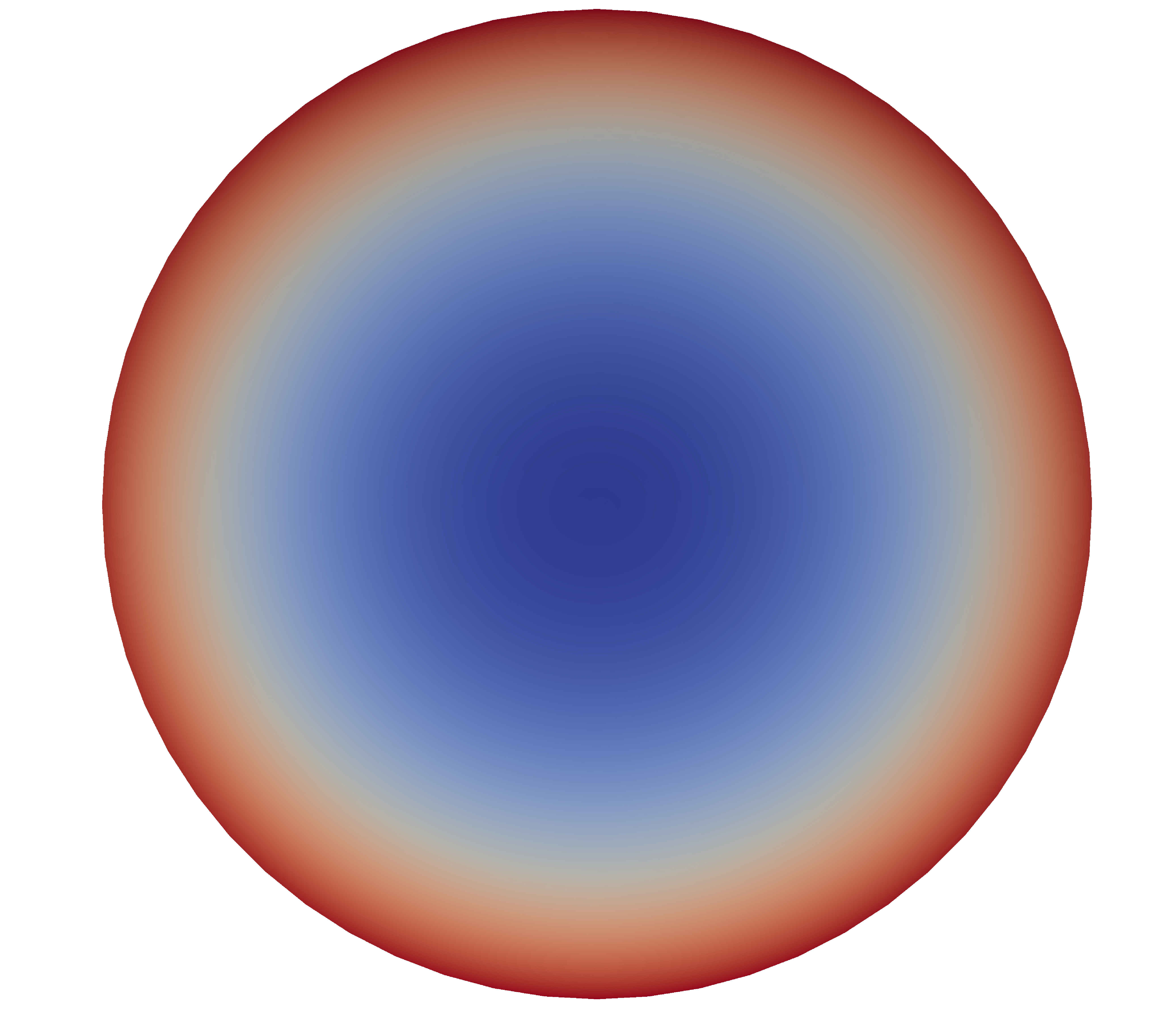 Figure 2
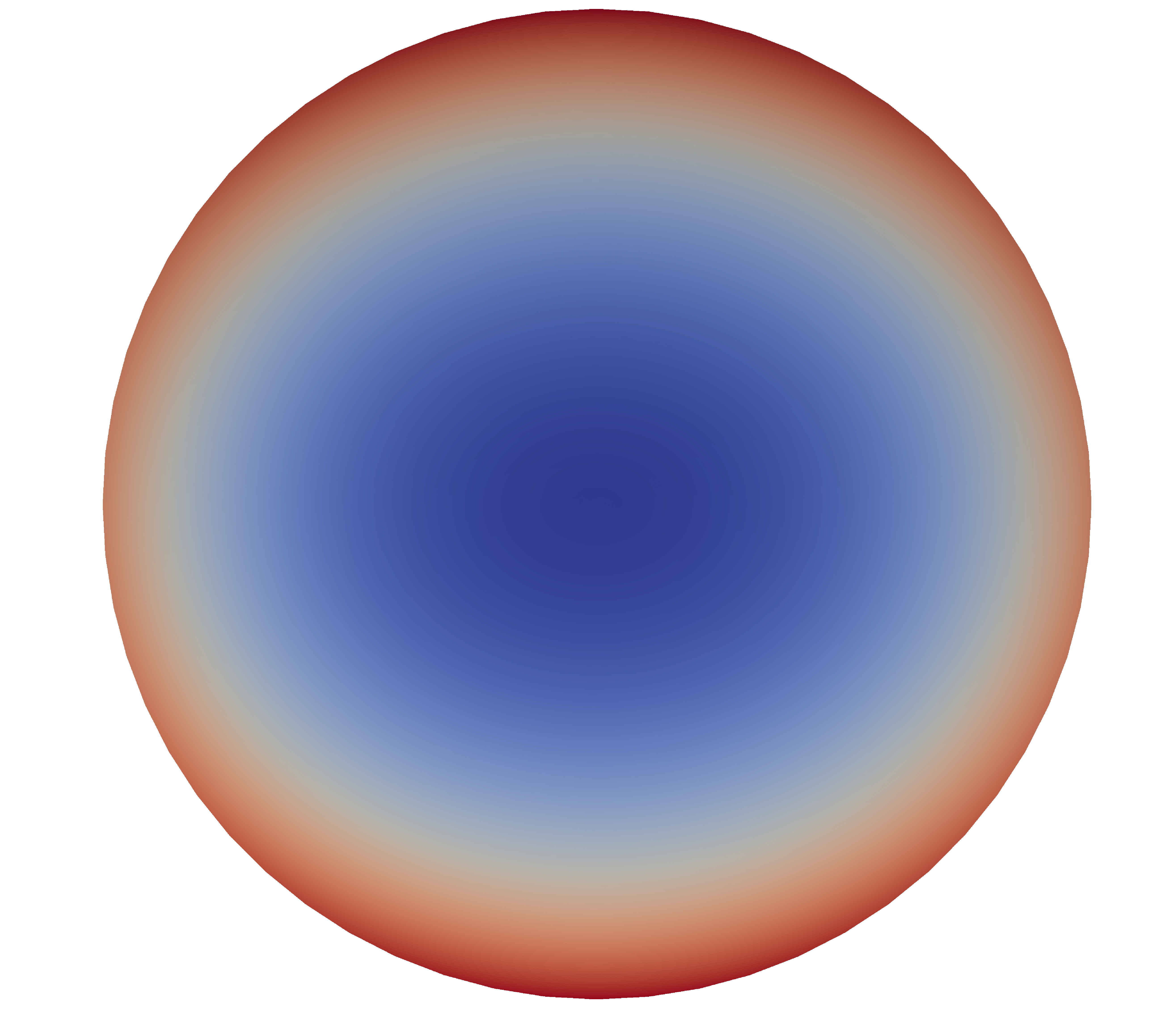 Figure 3
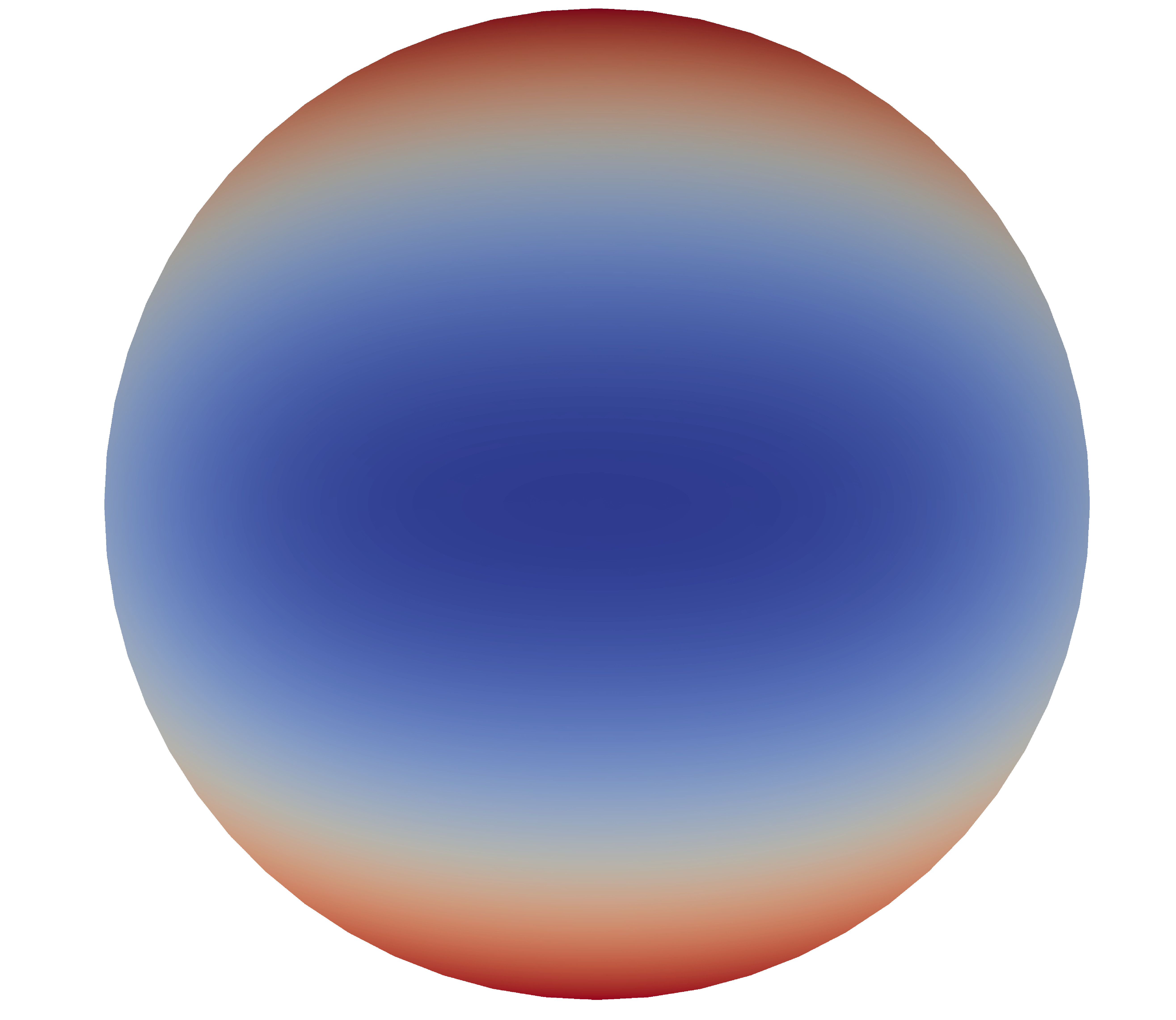 Figure 4
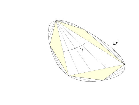 Figure 5
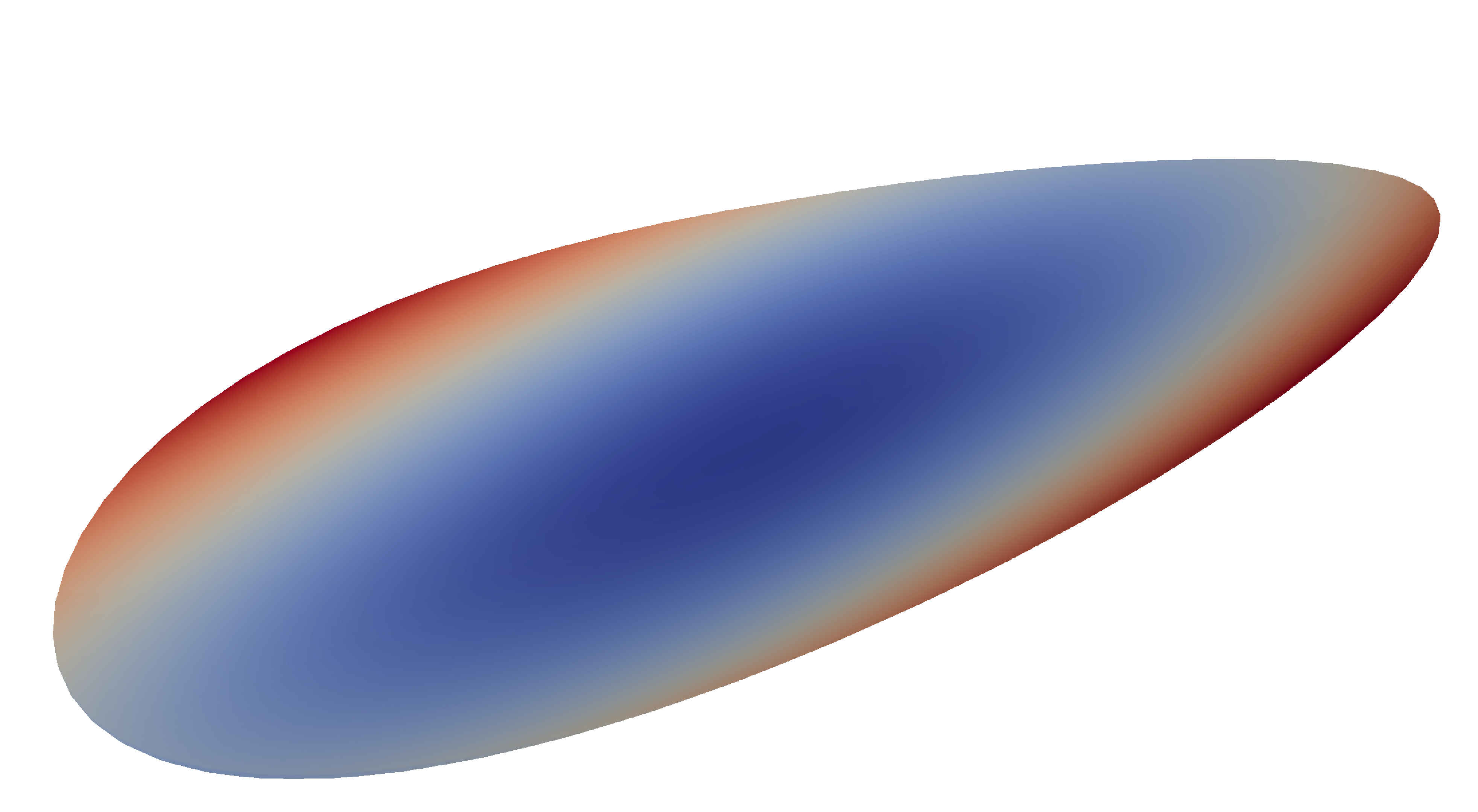 Figure 6
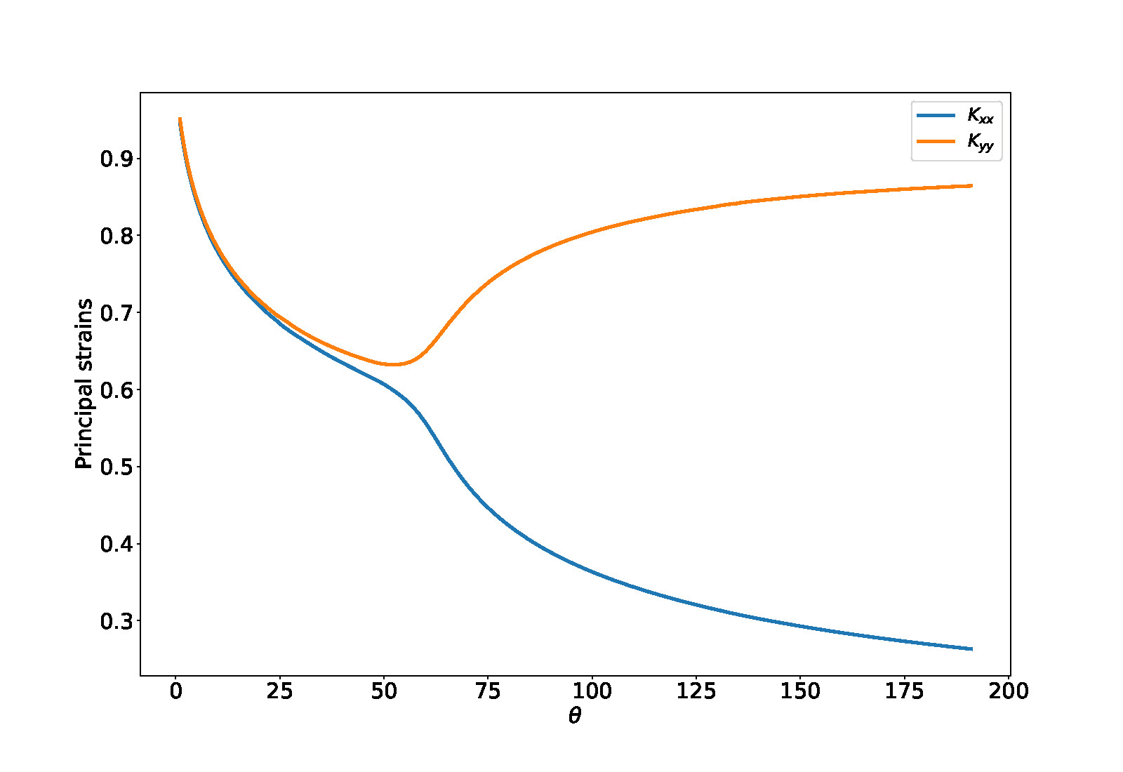 Figure 7
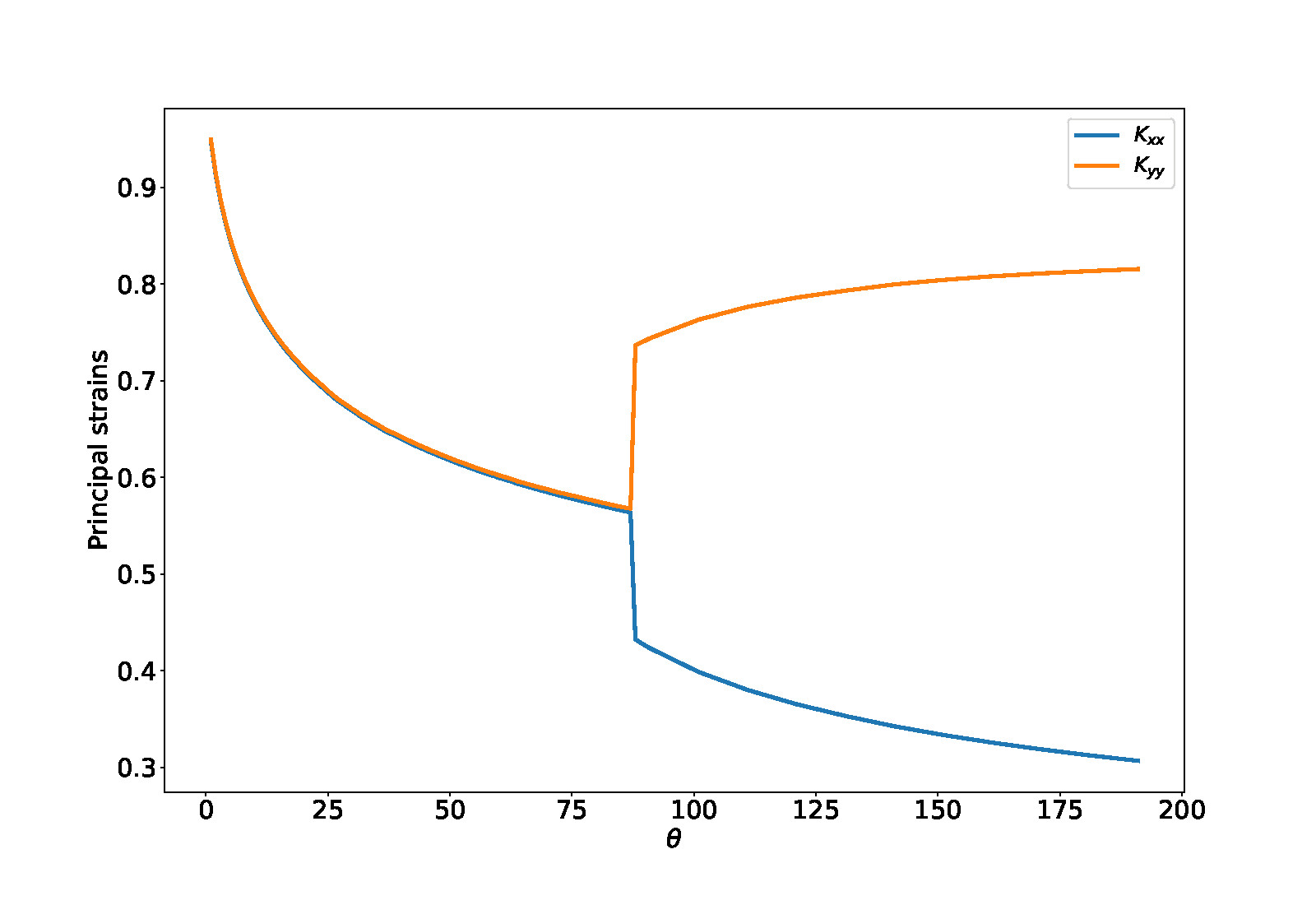 Figure 8
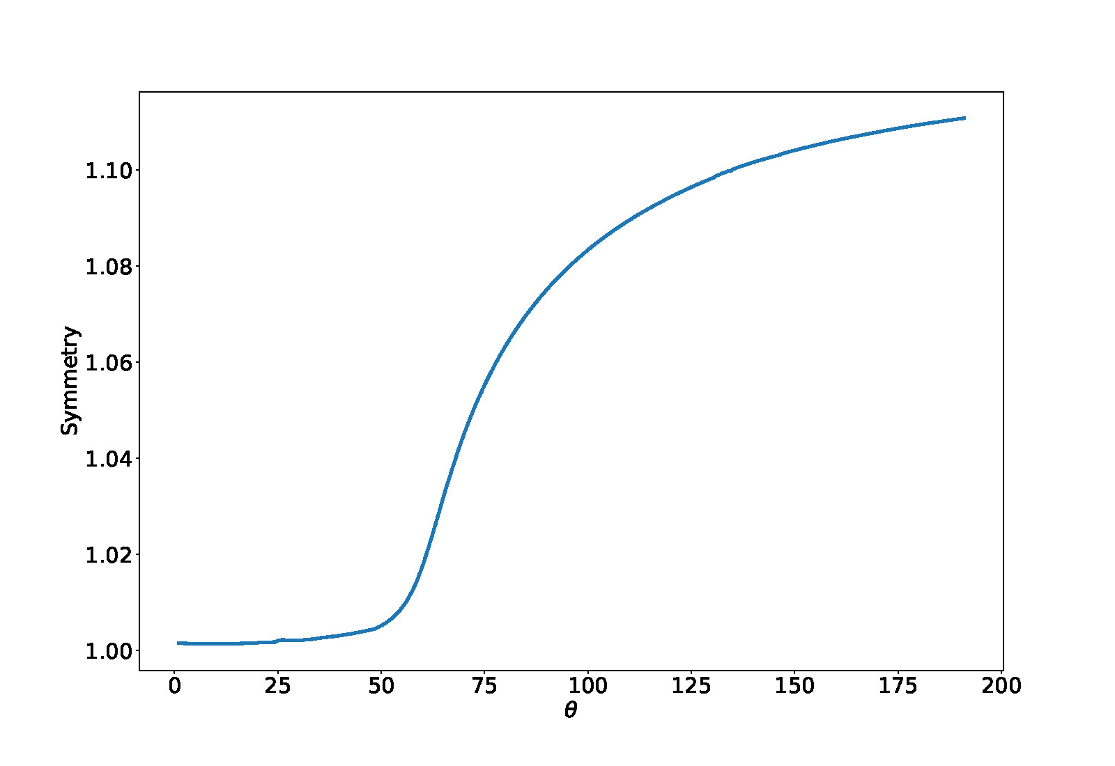 Figure 9
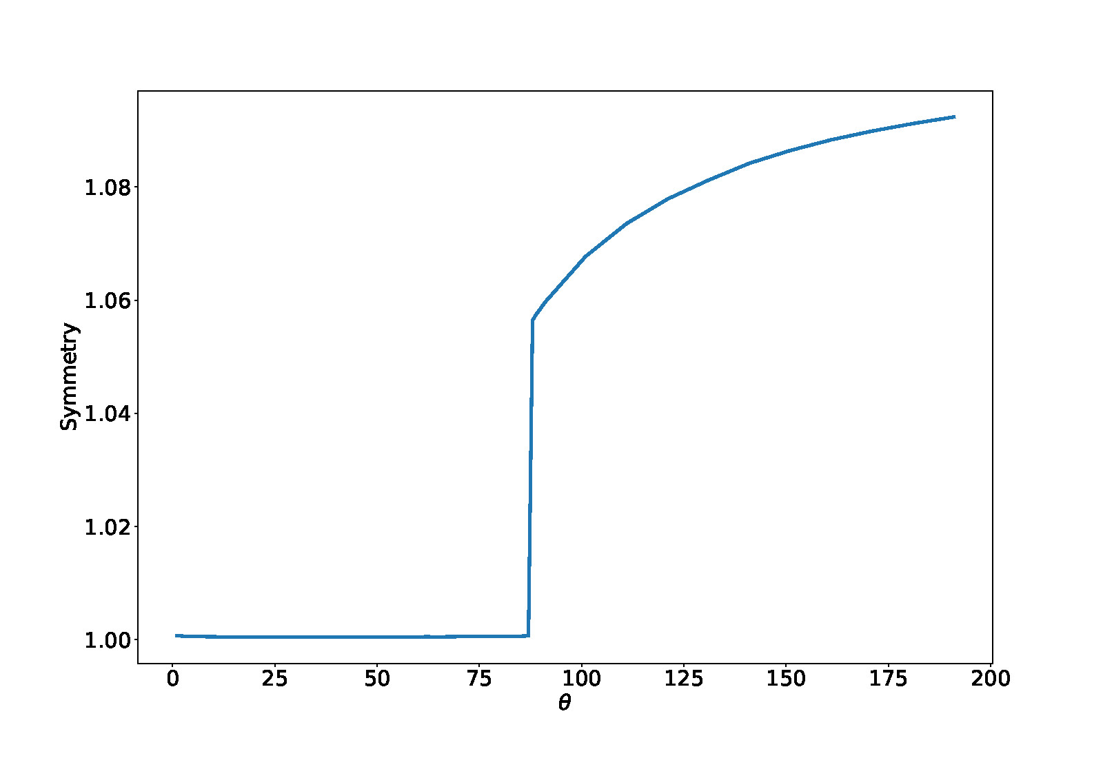 Figure 10
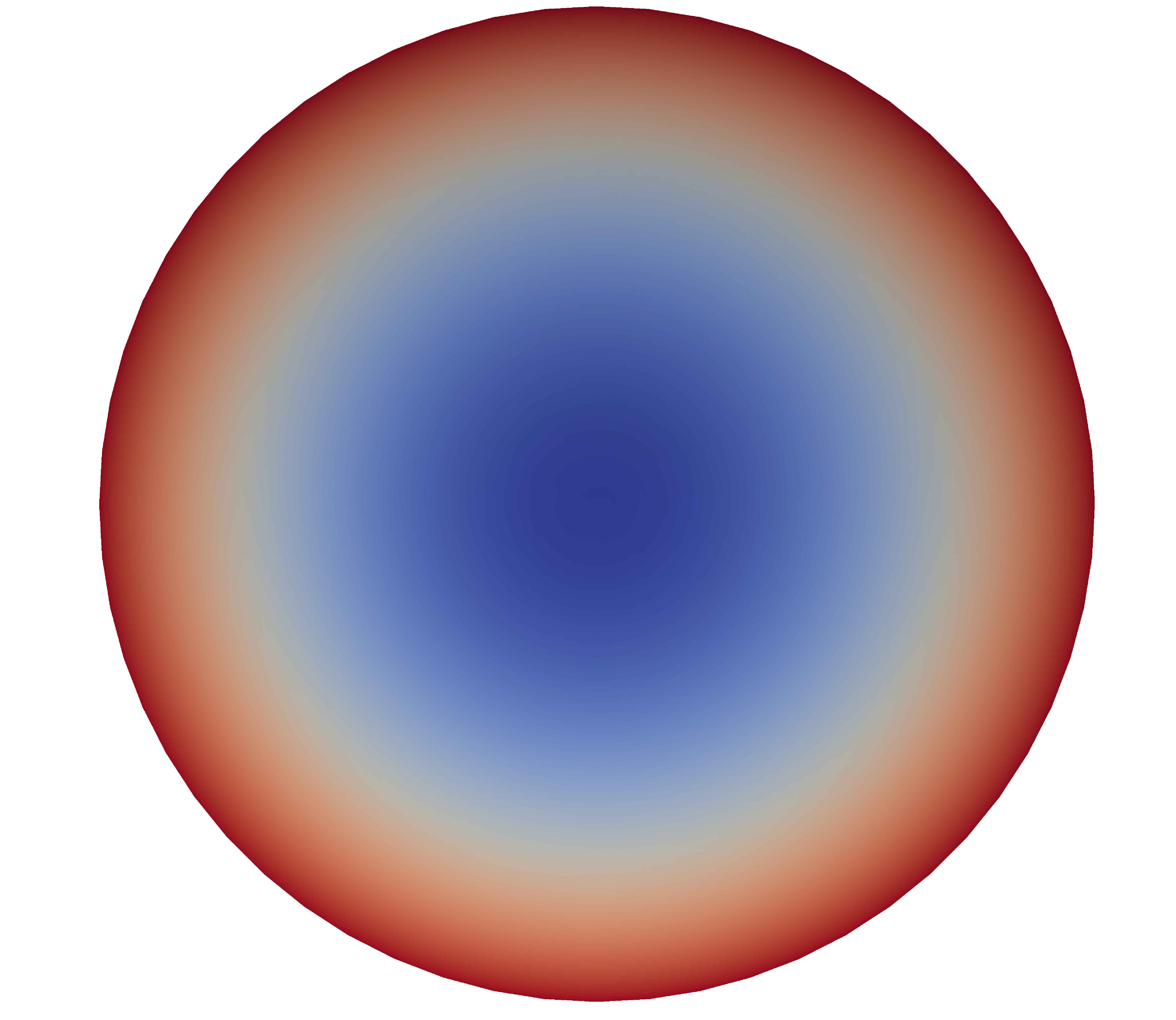 Figure 11
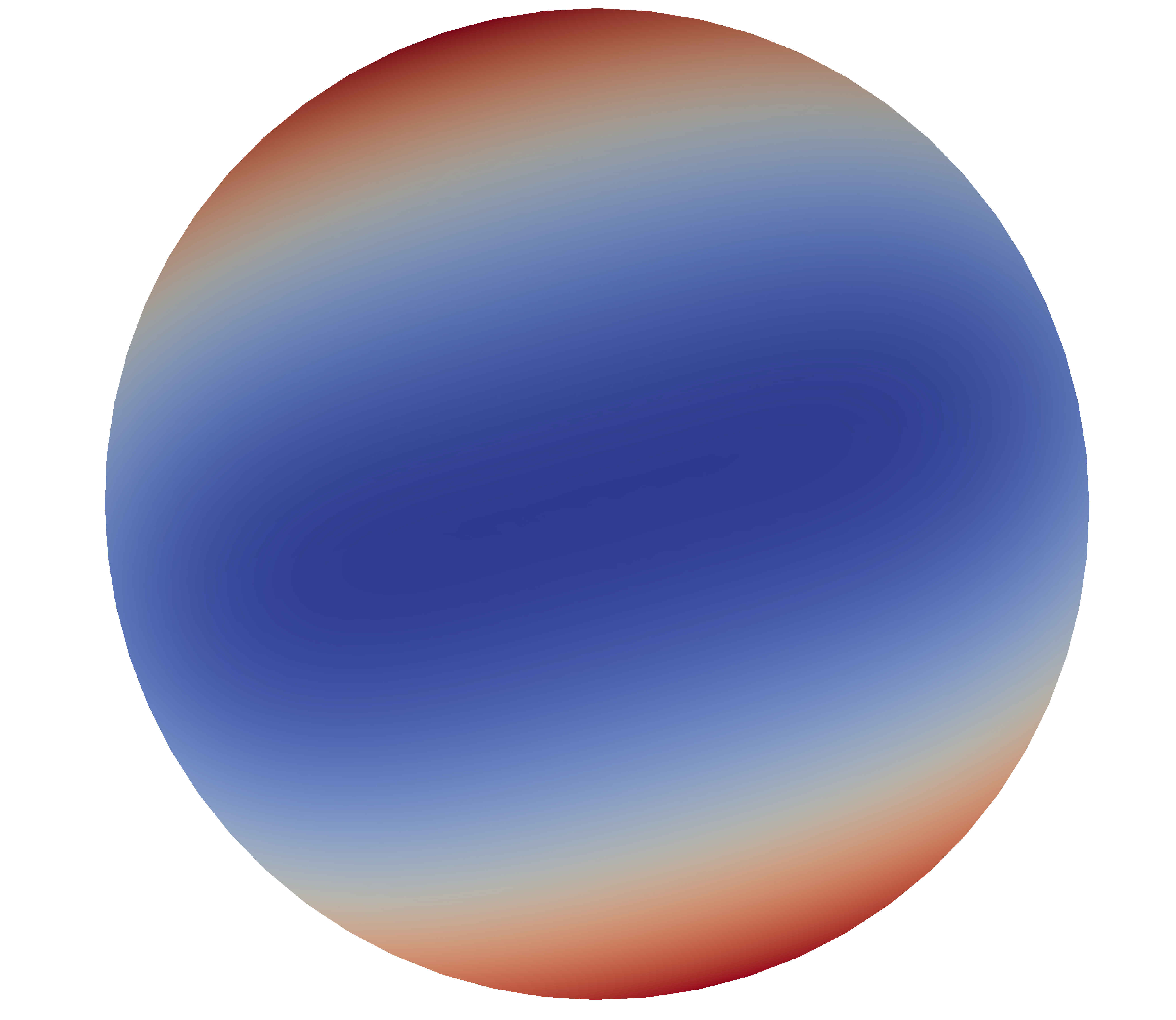 Figure 12
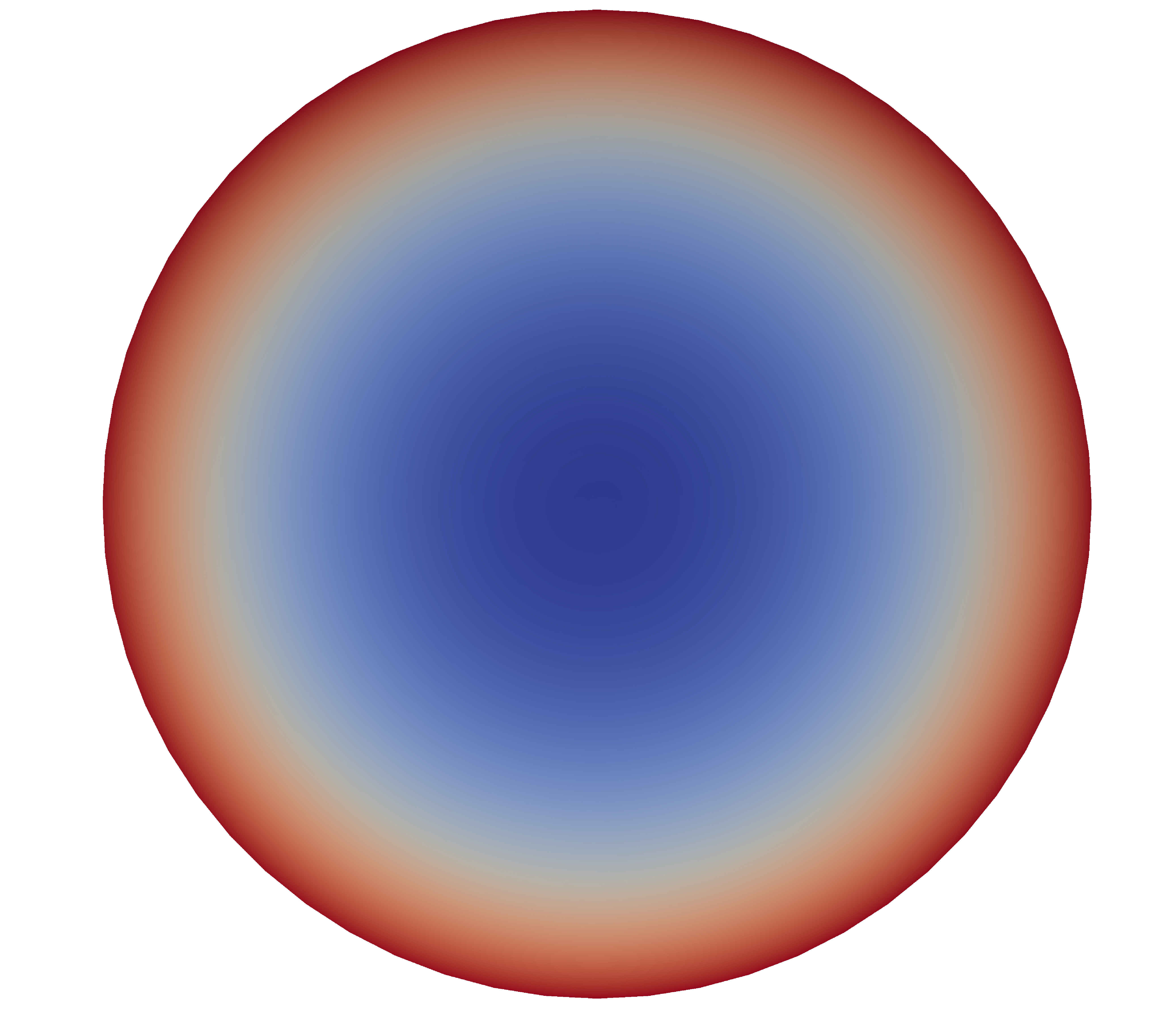 Figure 13
 Figure 14
Peer Reviews
No public reviews on file for this paper yet. If you reviewed it on a platform where reviews are public (OpenReview, ICLR, NeurIPS, ICML), you can paste yours below so the community can read it here.
Code & Models
Videos
No videos yet. Explain this paper in a talk, walkthrough, or lecture? Add one.
Taxonomy
TopicsAdvanced Mathematical Modeling in Engineering · Structural Analysis and Optimization · Elasticity and Material Modeling
Energy minimising configurations of pre-strained multilayers
Miguel de Benito Delgado111Universität Augsburg, Germany, [email protected] and Bernd Schmidt222Universität Augsburg, Germany, [email protected]
March 2, 2024
Abstract
We investigate energetically optimal configurations of thin structures with a pre-strain. Depending on the strength of the pre-strain we consider a whole hierarchy of effective plate theories with a spontaneous curvature term, ranging from linearised Kirchhoff to von Kármán to linearised von Kármán theories. While explicit formulae are available in the linearised regimes, the von Kármán theory turns out to be critical and a phase transition from cylindrical (as in linearised Kirchhoff) to spherical (as in von linearised Kármán) configurations is observed there. We analyse this behavior with the help of a whole family of effective von Kármán functionals which interpolates between the two linearised regimes. We rigorously show convergence to the respective explicit minimisers in the asymptotic regimes and . Numerical experiments are performed for general which indicate a stark transition at a critical value of .
Contents
1 Introduction
The topic of this paper is motivated by experimental observations on optimal energy configurations in thin (heterogeneous) structures with a pre-strain. The simplest example of such a structure is the classical bimetallic strip which consists of two strips of different materials with different thermal expansion coefficients joined together throughout their length. If heated or cooled, due to the misfit of equilibria, internal stresses develop. The flat reference configuration is no longer optimal and the strip bends in order to reduce elastic energy. This behavior can effectively be modelled with a 1d energy functional comprising a temperature dependent spontaneous curvature term.
In this paper we will investigate thin layers whose two lateral dimensions are much larger than their very small height and whose flat reference configuration is subject to internal stresses (one speaks of pre-strained or pre-stressed bodies). Examples of such structures are heated materials (with inhomogeneous expansion coefficients as in the bimetallic strip referred to above or homogeneous materials with a temperature gradient), crystallisations on top of a substrate as in epitaxially grown layers, or biological materials whose internal misfit is caused by swelling and growing tissue. Our main focus will be on multilayered heterogeneous plates, for which the effective plate theories have been provided in [11]. Our findings, however, apply equally to different situations as long as they are described by the same effective functionals, cf. Remark 1 below.
As a matter of fact, the situation is much more complicated and interesting for two dimensional plates than for one dimensional strips. It has been found that the assumed shape depends on the strength of the pre-strain and the aspect ratio of the specimen: Large pre-strains in very thin layers tend to cause cylindrical shapes whereas smaller pre-strains in thicker layers lead to spherical caps, [25, 31, 13, 14, 21, 12]. To explain this observation one argues that locally the energy is best released if a spherical shape is assumed. If, however, the aspect ratio is very small, i.e., the lateral dimensions are very large compared to the thickness, then this leads to geometric incompatibilities: non-zero Gauß curvature introduces a change of the metric which by far has too high elastic energy. In contrast, cylindrical shapes do not lead to such incompatibilities.
A thorough theoretical understanding of this mechanism through which ‘misfit’ of equilibria is converted into mechanical displacement is not only interesting from a mathematical point of view. In view of applications it has proved to constitute a convenient and feasible method to access and manipulate objects even at the nanoscale. By way of example we mention experiments on the self-organised fabrication of nano-scrolls, as reported in [34, 18, 27].
The aim of this paper is to shed light on the geometry of energetically optimal configurations of pre-strained heterostructures with the help of two-dimensional plate theories. More precisely, we consider effective plate theories for multilayers with reference configuration , , whose (small) misfit pre-strain is described by a matrix , scaling with .
The particular case with a misfit of the order of the aspect ratio has been investigated in [32, 33, 7]. The appropriate plate theory is the nonlinear Kirchhoff theory (in the finite bending regime) and energy minimizers turned out to be (portions of) cylinders whose possible winding directions and radii are determined explicitly. Therefore, in order to be able to encounter different behavior one has to consider weaker scalings of the misfit.
In [11] – based on the homogeneous case explored in [15] – we have found a whole hierarchy of effective plate theories for the scalings . Suitably rescaled, one obtains only three different limiting plate theories: the linearised Kirchhoff theory for , the von Kármán theory for and the linearised von Kármán theory for . With a view to our present investigation, we have moreover derived a fine scale in the critical von Kármán scale which interpolates continuously between the the two linearised theories.
For such small misfits one is lead to describe a deformation in terms of the scaled and averaged in-plane, respectively, out-of-plane displacements
[TABLE]
where unless and
[TABLE]
A limiting plate theory in terms of the limiting quantities is then derived as the -limit of the 3d nonlinearly elastic energy, rescaled by , cf. [11]. For a minimizer of the limiting theory one obtains the shape of an optimal configuration at finite : After descaling, its -averaged displacement is given approximately by
[TABLE]
Since , the in-plane components are indeed much smaller than the out-of-plane component. In his sense, the shape is to leading order described by only.
In the linearised regimes our results give the following picture: If , degenerate parabolas (infinitesimal parts of cylinders) are seen to be optimal, whereas for , non-degenerate parabolas (infinitesimal parts of an elliptical cap) are energy minimizers. Only in the latter case, however, the minimizer is unique (up to affine terms). Yet, even in case it turns out the geometric shape is uniquely determined as an infinitesimal part of a cylinder while the winding direction and radius may have several optimal values. In both cases we explicitly determine these minimizers. A basic observation shows that for these configurations are still asymptotically optimal in the ‘almost linearised’ regimes and , respectively.
The von Kármán regime is much more subtle. We focus on a prototypical functional in order to understand better the material response if the misfit (and hence ) is increased from [math] to a finite value. We show that for finite, although small, values of there is a unique branch of global minimizers emanating from a spherical cap. For a further study for general values of we then rely on computer experiments. To this end, we develop a penalised, nonconforming finite element discretisation using elements and employ projected gradient descent to solve the ensuing nonlinear problems while ensuring constraints are met. We first show -convergence of the discrete problems to the continuous one, then investigate the minimizers in their dependence on . Interestingly, our results seem to indicate a stark change of material response at a critical value of , showing a symmetry breaking ‘phase transition’ from a nearly spherical cap to an approximate cylinder.
Outline
We begin by recalling our main results from [11] in order to provide the appropriate plate theories in Section 2. There we also identify the effective elastic moduli and spontaneous curvature terms explicitly so as to transform the problem into a more amenable form to identify minimizers. We then discuss the linearised regimes and as well as the asymptotic von Kármán regimes and in Section 3. The structure of minimisers for small is investigated in Section 4. Finally, Section 5 contains our numerical findings.
2 Effective plate theories
We first recall the main results of our contribution [11] on a hierarchy of plate theories for pre-strained multilayers derived from non-linear three dimensional elasticity by -convergence. We then determine the effective (homogenised) elastic moduli and corresponding quadratic energy desnities of the plates in terms of the moments of the pointwise elastic constants of the layers.
2.1 Dimension reduction for pre-strained multilayers
Working exactly in the setting of [11] we consider a thin domain
[TABLE]
where is bounded with Lipschitz boundary, , subject to a deformation . Changing variables form to we obtain a deformation mapping and the energy per unit volume
[TABLE]
where the elastic energy density depends on a scaling parameter and is given by
[TABLE]
for , describing the internal misfit and the stored energy density of the reference configuration. For we include an additional parameter controlling further the amount of misfit in the model:
[TABLE]
We take fulfilling the usual assumptions of smoothness around , frame invariance, boundedness and quadratic growth which are detailed in [11]. After linearising around the identity, one obtains the Hessian
[TABLE]
for and defines by minimising away the effect of transversal strain on :
[TABLE]
for , , and has as its upper left submatrix and zeros in the third column and the third row. The functions , , are quadratic forms on which are positive definite on and vanish on antisymmetric matrices. Moreover, they satisfy the bounds
[TABLE]
for constants and a.e. . We also denote by the matrix which arises from by deleting its last row and last column. Then
[TABLE]
From and we define the effective form:
[TABLE]
and its relaxation
[TABLE]
In [11] it is shown that -converges for the convergence of the averaged in-plane and out-of-plane displacements in modulo a global rigid motion, cf. (1), to the following effective limiting functionals:
For the scaling as defined in [11] and convex , the linearised Kirchhoff energy is given by
[TABLE]
For we have the von Kármán type energy333As in [11] we slightly overload the notation in what would be a double definition of , using the letter in the subindex to dispel the ambiguity.
[TABLE]
Finally, in the regime we have the linearised von Kármán energy
[TABLE]
Remark 1
The precise assumptions on from [11] are not essential for the results of the present contribution. In what follows we will only need that the , , are quadratic forms on that vanish on antisymmetric matrices and satisfy (2) and that satisfies (3).
The existence of minimizers of (5) (6) and (7) follows by a standard application of the direct method or, in the setting of [11], as a direct consequence of -convergence and compactness.
Example. For a homogeneous material with linear internal misfit one has
[TABLE]
for , respectively, . These functionals, where the elastic coefficients do not depend on the out-of-plane component, can model for instance a single-layer material under thermal stress. In Section 5, we will study the energy (8) as a function of .
2.2 Effective moduli and minimising strains
This subsection serves to give explicit formulae relating the homogenised effective elastic moduli found above to the zeroth, first and second moment in of the individual . We also identify their pointwise minimiser so as to rewrite the effective quadratic forms in their most convenient form. The computations are completely elementary, we indicate the main steps.
Because vanishes on antisymmetric matrices we may restrict our attention to . From now on, we identify matrices with vectors in via
[TABLE]
and analogously , , . Then, for each there exists some symmetric, positive definite matrix such that for all :
[TABLE]
We define the moments of as
[TABLE]
It is easy to see that (2) implies that and are positive definite. We claim that also
[TABLE]
is positve definite. To see this, fix and note that for all
[TABLE]
since \big{(}tM^{1/2}(t)-M^{1/2}(t)\Lambda\big{)}x=0 for a.e. would imply that in contradiction to having at most two eigenvalues. Expanding the square we get
[TABLE]
and, choosing ,
[TABLE]
Let be given as in (2.1). Elementary calculations show that
[TABLE]
where
[TABLE]
We define the linear mappings , , by
[TABLE]
and the positive definite quadratic forms and on by
[TABLE]
In terms of these quantities our computation reads
[TABLE]
with
[TABLE]
Minimizing out yields
[TABLE]
3 Optimal configurations in the linearised and the asymptotic critical regimes
In this section we develop a characterisation of minimisers for the lower range and for the upper range of scalings. Recall from the discussion in Section 1 that we are primarily intested in the shape of the out-of-plane component . The results indicate that the characteristic shapes in the limit are (infinitesimal) cylinders and paraboloids respectively. Invoking the -convergence results with respect to the interpolation parameter from [11, Section 6] this will also shed light on the optimal shapes in the asymptotic regimes and for the von Kármán scaling . We collect our results in the following three theorems, where indeed Theorem 1 is indeed rather an elementary observation based on our preparations form the previous section and Theorem 3 is a direct consequence of [11, Section 6]. We allow for a general bounded Lipschitz domain in these theorems.
Theorem 1
The minimisers of , eq. (7), are of the form
[TABLE]
with the constants from (13). is unique up to an infinitesimal rigid motion and up to the addition of an affine transformation.
Theorem 2
Up to the addition of an affine transformation, the minimisers of , eq. (5), are of the form
[TABLE]
where are given in (11) and (13), respectively.
Remark 2
Describing symmetric matrices by vectors as in Section 2.2, the set is the set of touching points of the two quadrics (a cone) and (an ellipsoid), where with . If , intersecting with an affine plane containing three distinct points of shows that is an ellipse and then even . This shows that either and there is a unique minimizer, or and there are precisely two minimizers, or is an affine ellipse and to each ‘winding direction’ , , there is a unique curvature such that .
Theorem 3
Suppose that are minimisers of , eq. (6).
- a)
As , up to infinitesimal rigid motions in the in-plane component and up to the addition of affine transformations in the out-of-plane compenent, in with as in (15). 2. b)
As , up to the addition of affine transformations in the out-of-plane component and up to passing to a subsequence, in with as in (16).
**Proof of Theorem 1 ** By (7) and (12)
[TABLE]
with and is minimal (with value ) if and only if and a.e.
**Proof of Theorem 3 ** a) is immediate from [11, Theorems 7,10,11]. b) directly follows from [11, Theorems 7,8,9] if is convex. For general first note that the compactness result in [11, Theorem 7] does not use convexity, so that in for some . Now fix and . Since , the function satisfies . Also choose with , cf. (12) and (13). Then for we have by (14)
[TABLE]
With the help of the Vitali covering theorem we can exhaust up to a set of negligible measure with disjoint convex subdomains . Denoting the accordingly restricted functionals by , we have
[TABLE]
where we have made use of the lower bound in the -convegence of to , see [11, Theorem 8], in the third step and of Theorem 2 in the fourth step. So we must have for all and hence a.e. on and so the claim follows from Theorem 2.
As for Theorem 2, it is straightforward to see that as defined in the theorem is a minimisers of . However, the proof that every minimiser of is necessarily of this form needs some work. The difficulty lies in excluding the possibility of constructing a minimiser by piecing together functions whose Hessian belongs to the set , all with minimal energy but lacking a nice global structure. Yet it is possible to obtain a global representation of the Hessian which shows that it must be constant over so that minimisers are (up to an affine transformation) indeed cylindrical. In order to do this we require (cf. [28]):
Definition 1
Let a convex bounded domain and be an isometry. A connected maximal subdomain of where is constant and is affine whose boundary contains more than two segments inside is called a body. A leading curve is a curve orthogonal to the preimages of on the open regions where is not constant, parametrised by arc-length. We define an arm to be a maximal subdomain which is covered (parametrised) by some leading curve as follows:
[TABLE]
where . We also speak of a covered domain.
The existence of covered domains for isometric immersions is shown in [28, Corollary 1.2].
Proposition 1
Let and . There exists a neighbourhood of such that, if a.e. in , then for a suitable there exist maps and such that and
[TABLE]
if .
Proof.
We may without loss of generality assume that is convex. Using [15, Theorem 10] take such that , on and . By scaling with we can extend to an isometry ([15, Theorem 7]) with . Then, because is an isometry:
[TABLE]
where is the normal and the second fundamental form of the surface . Since a.e. near , there is a neighbourhood of covered by some leading curve , that is: and, by [33, p. 111], on we have
[TABLE]
with . Now, [19, Proposition 1, eq. (12)] shows that is independent of , hence is also independent of and we can subsume it into the function . Setting we obtain the representation (17). ∎
Finally, we come to:
**Proof of Theorem 2 ** To recapitulate, according to (5) and (14) the linearised Kirchhoff energy is given by
[TABLE]
for (and otherwise).
We observe first that the set is not empty because is non-negative and strictly convex, but it also need not consist of just one point. Note next that is a minimiser of (18) iff for almost every : On the one hand, every minimiser has finite energy and thus must be pointwise a.e. in the set . On the other, any function with a.e. minimises the integrand in (18) pointwise and thus the energy.
Next we show that any two elements of are linearly independent. Indeed, by strict convexity we have for all :
[TABLE]
Hence or else would not be minimisers. Because attains a lower value here we must have . But then it cannot be that for any scalar or else it would hold that , a contradiction. Consequently, we have in particular unless . But in that case and the proof would be concluded.
Let now be a minimiser for . Note first that cannot be constant over open sets: indeed we just saw that w.l.o.g. and consequently the condition is excluded for a minimiser on any set of positive measure. Consider then some point with a neighbourhood where is not constant and use the representation (17). We have that, pointwise a.e. and over :
[TABLE]
If , by varying we obtain distinct, linearly dependent matrices . Because a.e., this shows that for a.e. . As a consequence, must be constant. But then is also constant or again we would have points at which is linearly dependent. Since this holds locally around every , we deduce that is constant on and because we can cover in this manner, there exists such that a.e. over .
4 Structure of minimisers for
for small
The second main contribution of this work is a first study of the properties of minimisers in the interpolating regime, “close” to the linearised von Kármán model. The results in Section 3 show that the transition from spherical to cylindrical shapes occurs in the interpolated von Kárma\a’an as the strength of the misfit increases. We will see that for small indeed there exists a unique stable branch of solutions emanating from a perfect spherical cap at .
For the sake of clarity we restrict to the prototypical model from (8):
[TABLE]
Natural subsequent steps along this line of work, which we do not take here, are to consider the regime of large values of and to investigate the existence of the conjectured critical value , as well as to consider the full model derived in (6).444In Section 5 we conduct numerical experiments supporting the conjecture that this critical value exists.
We recall that the existence of minimizers is guaranteed, cf. Remark 1. Without loss of generality wee assume that the barycenter of is [math]. So with for a function we in particular have . In order to avoid ambiguities (and to apply Korn’s and Poincaré’s inequalities) we restrict the functions to lie in the Banach space
[TABLE]
with as in
[TABLE]
and norm . By the arguments in [11, Remark 2] working with these spaces does not lead to a loss of generality either: For an affine function , is a symmetrised gradient.
For small values of the parameter we have the following structural result on the set of minimizers showing the existence of a smooth branch of unique global minimisers. Let with .
Theorem 4
There exists an , a unique point and a uniquely determined map such that and for each :
[TABLE]
The proof is a direct consequence of Theorems 5 and 6 that are proved in the following two subsections. The main difficulty in obtaining a local branch of minimizers for lies in the fact that minimisers at are not unique. Indeed,
[TABLE]
as can be readily checked. This is addressed in Subsection 4.1. The proof that in fact these minimisers are global is achieved by an application of a Taylor expansion for a carefully perturbed functional in Subsection 4.2.
4.1 A branch of solutions for
**Notation **
In this section, the parameter will be explicitly included in the arguments of the functional and differentiation is understood to be with respect to the variables , unless otherwise stated, i.e.
[TABLE]
We are interested in the existence and uniqueness of solutions to the equation
[TABLE]
as a function of with given by (8). We will in fact prove the existence of a point such that there exists a (locally) unique function , starting for at , such that every is a critical point for . However, lack of uniqueness of minimisers at , (19) will thwart what would be a natural application of the implicit function theorem. The problem manifests itself as a lack of injectivity of the first derivative at
[TABLE]
which for is
[TABLE]
and this vanishes at every and the unique , , such that and , i.e., . Because of this the equation
[TABLE]
cannot be uniquely solvable for as a function of , even locally. Nevertheless, after some computations one can see that the problem is the presence of a leading factor which we can dispense with, because we may apply the implicit function theorem to the set of equivalent equations
[TABLE]
These equations are equivalent to for any and by an application of the implicit function theorem around a specific point we determine the existence of a solution function with open, and . Then we have for because of the equivalence mentioned and by the choice of .
Theorem 5
There exists an open set in , an , a point such that and a uniquely determined map such that and
[TABLE]
for all and .
Proof.
We first define a new set of equations to solve, then show that the second derivative of is one to one and then the conclusion is exactly that of the implicit function theorem. For brevity we write
[TABLE]
These define a scalar product and a norm in since is by construction bilinear and symmetric and it is positive definite on this space. Even though vanishes on antisymmetric matrices, during the proof we keep track of symmetrised arguments to these functions for the sake of clarity.
Step 1: Equivalent equations.
From the computations leading to (20) we have:
[TABLE]
and
[TABLE]
for all . We observe first that, because is independent of the right hand side makes sense even if . Now, on the one hand, for any fixed value of solving the system
[TABLE]
implies solving:
[TABLE]
where is given by
[TABLE]
On the other hand, solving for is equivalent to solving the original problem as we desired.
Step 2: A zero and the derivative of .
Since we are interested in the behaviour around , we evaluate here and obtain
[TABLE]
We can compute a zero of by first considering the last term, which vanishes for all if and only if . We next observe that the first term encodes the orthogonality of to the space of symmetrised gradients with respect to the scalar product induced by . The realizing this is attained by projecting onto , i.e.
[TABLE]
where is the orthogonal projection onto given by
[TABLE]
By the Korn-Poincaré inequality this determines uniquely. We have then a point such that
[TABLE]
Finally, we compute to have the derivative of :
[TABLE]
Step 3: The map is an isomorphism.
Note first that the map
[TABLE]
defines a scalar product in , with positive-definiteness following from Korn-Poincaré’s and Poincaré’s inequality. Then we can write as
[TABLE]
where we defined , a continuous map from to . The Riesz representation for in is then and the map
[TABLE]
is clearly an isomorphism in , with continuity for following from the continuity of and the Sobolev embedding . ∎
4.2 Uniqueness and globality of minimisers
In addition to the previous local result, we can prove that the critical points found in the previous subsection are the unique global minimizers for small non zero values of the parameter . We do this in two steps: close to the origin of the branch of solutions, we would like to perform a Taylor expansion and use that the second differential at is “almost” positive definite.
The key idea is to slightly modify the energy by a shift and a rescaling in order to obtain derivatives as those appearing in the equivalent equations (22) of Theorem 5, thus obtaining a positive definite second derivative. We set
[TABLE]
and then is a minimiser of if and only if is a minimiser of . In other words, if is a minimiser of , then and minimise .
We name the point around which we investigate the modified functional:
[TABLE]
Theorem 6
There exists and a neighborhood with such that for every , every critical point of is the unique global minimiser of .
Proof.
We proceed in three steps. First we prove that there is some such that is positive definite for all if for some suitable and as defined in (23). Then we use this to determine a neighbourhood of where (local) minimisers of will be global by first considering points close to one such minimiser and finally those far away. We will need the first two derivatives of .
For the first differential we apply the chain rule to obtain and substitute:
[TABLE]
For the second differential we can compute another directional derivative:
[TABLE]
Step 1: Local positive definiteness.
We show there exist and s.t. is positive definite for all and all . More precisely, we even show that there exists some such that
[TABLE]
for all , and .
Let then be fixed and to be determined later and let with . We start by bringing terms together in (24):
[TABLE]
Given we have, by the bounds (2) for and Hölder (with the Sobolev embedding ):
[TABLE]
Using this, the first and last term above can be estimated using Korn-Poincaré and Poincaré’s inequality:
[TABLE]
for constants , where in the last step we used the assumption to bound by some constant independent of . For the second term, use Cauchy-Schwarz for , and the same ideas as above:
[TABLE]
Again, we used that by assumption and .
Finally we estimate the third term in with analogous arguments and obtain , for a . Bringing the previous computations together, with a we have:
[TABLE]
from which (25) follows if and are chosen sufficiently small.
From now on, we let be a critical point of with
[TABLE]
and we prove that it is in fact the unique global minimizer.
Step 2: Estimates close to .
Consider first some which is close to :
[TABLE]
With a Taylor expansion and (25) we see:
[TABLE]
[TABLE]
Step 3: Estimates far away from .
Consider now any with
[TABLE]
which by (26) implies that . We consider two cases:
Case 1: : We discard the first term in the energy, recall that and use the lower bound for in (2) and Poincaré’s inequality:
[TABLE]
for a . To compare this with the energy at we add and subtract :
[TABLE]
where the last line is due to the fact that minimises over the ball .
Case 2: : In this case we also have by (26) and (28). We can estimate the energy for as follows:
[TABLE]
where we used the Cauchy-Schwarz inequality with . Both terms may be estimated once again by a combination of the bounds (2) for , Sobolev’s embedding and Poincaré’s inequality:
[TABLE]
and
[TABLE]
since . Now plug this back into the previous estimate and insert
[TABLE]
to obtain
[TABLE]
As above, the last line holds because minimises in a -neighbourhood of itself. ∎
5 Discretisation of the interpolating theory
Our goal in this section is to study the qualitative behaviour of minimisers in the interpolating regime . To this end, we develop a simple numerical method to approximate minimisers and prove -convergence to the continuous problem. Numerical computations are then conducted for the prototypical example from (8). We experimentally evaluate the conjectured existence of a critical value for which the symmetry of minimisers is “strongly” broken. We will not provide a full theoretical analysis, but instead adduce some empirical evidence to support the claim.
As can only be expected from a topic originating in structural mechanics, numerical methods for plate models are a vast field with a long history and as such a comprehensive review falls well beyond the scope of this contribution. However, it can be said that a significant portion of finite element approaches focus on the Euler-Lagrange equations. For von Kármán-like theories like our interpolating regime, these are transformed into an equivalent form in terms of the Airy stress function [20, §2.6.2]. The resulting system of equations is of fourth order and can be solved with conforming elements like Argyris or specifically taylored ones. To avoid the higher number of degrees of freedom, non-conforming methods can be used instead,555See [23, 24] for particular instances of a conforming and a non-conforming method respectively, as well as reviews of recent literature. but a poor choice of the discretisation can suffer from locking, as briefly described in Remark 4. Some successful classical methods employ Discrete Kirchhoff triangles (DKT), but it is also possible to employ standard Lagrange elements with penalty methods [8], as we will do.
A recent line of work, upon which we heavily build in this section, is that of [4, 6], where the author develops discrete gradient flows for the direct computation of (local) minimisers of non-linear Kirchhoff and von Kármán models. -convergence and compactness results are also proved showing the convergence of the discrete energies to the continuous ones, as well as their respective minimisers.666For a concise introduction to -convergence for Galerkin discretisations and quadrature approximations of energy functionals, see [26]. Crucially, these papers use DKTs for the discretisation of the out-of-plane displacements, allowing for a representation of derivatives at nodes in the mesh which is decoupled from function values. This enables e.g. the imposition of an isometry constraint for the non-linear Kirchhoff model, but also the computation of a discrete gradient projecting the true gradient of a discrete function into a standard piecewise space. The operator has good interpolation properties circumventing the lack of smoothness of DKTs which would otherwise make them unsuitable to approximate solutions in . We refer to the book [5] for a systematic and mostly self-contained introduction to these methods.
5.1 Discretisation
We wish to investigate minimal energy configurations of the following functional:
[TABLE]
where , cf. (6). We recall the representation of derived in (12), which in particular shows that is a strictly convex polynomial of degree on . It is extended to a convex quadratic function on by our setting
[TABLE]
for . We assume that is a bounded simply connected domain with Lipschitz boundary and barycenter [math]. We implement (projected) gradient descent in a non-conforming method using linear Lagrange elements. The first step is to transform the problem into one of constrained minimisation reducing the order of the elements required.
Problem 1
Find minimisers of
[TABLE]
with and
[TABLE]
If , then we set .
Note that our assumptions on guarantee that . We can now use -conforming elements but, for simplicity of implementation, instead of adding the constraint into the discrete spaces to obtain a truly conforming discretisation, we add a penalty term to ensure that the solutions are close to gradients.
Assume from now on that is a polygonal domain. For fixed , introduce a quasi-uniform triangulation of with triangles of uniformly bounded diameter for some and all and .777 Note that this does not allow for arbitrary local refinements or grading (a different scaling of simplices along different directions as ), but the fact that this is not optimal is not of concern here. Such a mesh is in particular said to be, in virtue of the uniform upper bound, shape-regular. We denote by the set of all nodes of the triangulation. Define to be the standard piecewise affine, globally continuous Lagrange finite element space in two dimensions:
[TABLE]
Quadrature rules will be chosen to be exact for this polynomial degree and the first integrand in the energy interpolated for this to apply by means of the interpolated quadratic function
[TABLE]
This is defined (with a slight abuse of notation) component-wise using the element-wise nodal interpolant , defined for functions such that for all as
[TABLE]
where is the truncation by zero outside of the global basis function . Because this is a linear combination of truncated global basis functions, the range of is the space of discontinuous, piecewise affine Lagrange elements.
In cases where the function to be interpolated is continuous, the element-wise nodal interpolant coincides with the standard nodal interpolant into the space of globally continuous, piecewise affine functions, which is defined as
[TABLE]
Notice that the shape functions are not truncated. In order to control the error incurred by the interpolation. When working with discontinuous functions in , we will use the following local result. This follows from standard nodal interpolation estimates (see e.g. [17, Theorem 4.28] or [9, (4.4.4)])
[TABLE]
or can be shown directly, e.g. in [5, Proposition 3.1].
Lemma 1** **(Local interpolation estimate)
Let and . If is the element-wise nodal interpolant (30), then
[TABLE]
The goal is to solve:
Problem 2
Let . Compute minimisers of the discrete energy
[TABLE]
for . (As usual, if , we set .)
Remark 3** **(Scaling of the constants)
The penalty needs to explode as in order for the functionals to -converge (Theorem 7). However, large penalties negatively affect the condition number of the system, so that an adequate choice for , dependent on the mesh size , is required [17, p.416]. We have not explictly investigated how this requirement interacts with the -convergence of the functionals, but in our proof we require only that not faster than . In the implementation we use . Analogously, large values of the Lamé constants have a similar effect and therefore hinder convergence, so one needs to scale them to the order of the problem.
Remark 4** **(Common issues with FEM for plates)
Discretisations for lower dimensional theories can face complications due to the infamous locking phenomena. In a nutshell, these mean that as the thickness of the plate tends to zero, discrete solutions “lock” to stiff states of lower, or even vanishing, bending or shearing than the analytic ones.888We refer to [3] for a first rigorous definition of locking, to [29, Chapters 5 and 6] for detailed computations highlighting the issues with linear elements in the context of Timoshenko beams and to the thesis [30] for a thorough and detailed analysis of locking in shell models. Another instance of unexpected behaviour is known as the Babuška paradox [2], again a failure to converge as expected, which can happen in e.g. the Kirchhoff model when both vertical and tangential displacements are fixed at the boundaries of a polygonal domain: these so-called “hard” support constraints are not enforced in the same manner as in the continuous model because of the approximated domain.
There are two potential sources of locking in our setting: the penalty term , which is akin to the shear strain in Timoshenko beams, and . We have not obtained any a priori bounds on the error in this work, but a rigorous treatment of the problem would require estimates which are uniform in these parameters as the mesh diameter goes to zero. For the regimes studied and the geometries considered we have found the issue to be of moderate practical relevance, but it does manifest itself e.g. with more complicated domains or higher values of .
Finally, our simulations will not suffer from Babuška’s paradox because we do not prescribe boundary conditions.
5.2 -convergence of the discrete energies
The first step in the proof that is dispensing with the interpolation operators for numerical integration: due to the good properties of , we can assume that we work with the true integrals instead of :
Lemma 2** **(Numerical integration)
Let be uniformly bounded in and let as above. Let A_{\varepsilon}\coloneqq\big{(}\theta^{1/2}(\nabla_{s}u_{\varepsilon}+\tfrac{1}{2}z_{\varepsilon}\otimes z_{\varepsilon}),-\nabla z_{\varepsilon}\big{)}. Then, as :
[TABLE]
Proof.
By the local interpolation estimate Lemma 1:
[TABLE]
Now, the first term is simply which is uniformly bounded since , and for the second we use that both and are piecewise constant so that for ,
[TABLE]
and
[TABLE]
A standard inverse estimate (see e.g. [9, Theorem 4.5.11]) provides the bound
[TABLE]
We plug this into the preceding computation to obtain
[TABLE]
The last two norms being uniformly bounded, we conclude:
[TABLE]
∎
The second step is, as usual, to ensure that we can focus on smooth functions for simplicity in the construction of the upper bound:
Lemma 3
The set is -dense in .
Proof.
This follows from and the density of in . ∎
Theorem 7
Let be given by (29) and (32) respectively. Assume that such that as . Then as with respect to weak convergence in .
Proof.
Because of Lemma 2 we can substitute for in . Also, by Lemma 3 it is enough to consider smooth functions for the upper bound. Set
[TABLE]
Step 1: Upper bound.
Let be up to the boundary and define , where is the nodal interpolant of (31). Note that because and are smooth, we can apply standard interpolation estimates to show strong convergence in of these sequences towards and . By the compact Sobolev embedding we have in , and in , so we have that in . Since is a polynomial of degree 2, this implies
[TABLE]
as . By the same interpolation estimate above and the assumption on we have that as , and consequently
[TABLE]
Step 2: Lower bound.
Let with , and weakly in to . Because in , we have that in . Moreover, . If , the assertion is trivial. If not, then and for a subsequence . But then . Dropping the (non-negative) term in and by the weak sequential lower semicontinuity of all integrands involved ( being a convex quadratic function), we then get
[TABLE]
∎
The final ingredient of this subsection is a proof that sequences with bounded energy are (weakly) precompact. The fundamental theorem of -convergence then shows convergence of global minimisers. In order for this to work, we need to assume conditions in the space which provide Korn and Poincaré inequalities. We can do this using functions with zero mean, zero mean of the gradient or zero mean of the antisymmetric gradient as we do above, but including these conditions in the discrete spaces is not entirely trivial. Because the energies are invariant under the transformations which are factored out by taking quotient spaces as described in the sections mentioned, it is enough for our purposes to claim compactness modulo these transformations and to exclude them in the implementation via projected gradient descent.
Theorem 8** **(Compactness)
Let be a sequence in with bounded energy. Then there exist such that and . in .
Proof.
As above, let A_{\varepsilon}\coloneqq\big{(}\theta^{1/2}(\nabla_{s}u_{\varepsilon}+\frac{1}{2}z_{\varepsilon}\otimes z_{\varepsilon}),-\nabla z_{\varepsilon}\big{)}. Note that we cannot use Lemma 2 to substitute for since we do not have uniform bounds in by assumption, so we work directly with .
We begin by observing that, as is a convex quadratic function bounded from below which is strictly convex on , there are constants such that
[TABLE]
for all . In particular,
[TABLE]
and consequently, by Poincaré’s inequality:
[TABLE]
We have then a subsequence (not relabeled) weakly converging in to some . In particular and in . But also
[TABLE]
and therefore , i.e. .
Now, for the sequence we must work with instead. First write
[TABLE]
and thus
[TABLE]
Since this applies pointwise, after (local) interpolation the estimate still holds:
[TABLE]
where in the firs step we have used that is piecewise constant. So
[TABLE]
We claim now that . Indeed, by the local interpolation estimate (Lemma 1) and Hölder’s inequality for integrals and for sums:
[TABLE]
and this goes to zero as by (33). But then and by Korn-Poincaré’s inequality, the Sobolev embedding and the previous bound, we have
[TABLE]
The sequence is therefore also weakly precompact in and the proof is complete. ∎
5.3 Discrete gradient flow
As a concrete example we specialize now to the prototypical example
[TABLE]
cf. (8). For each discrete problem, we compute local minimisers using gradient descent, for which the basic result is the following (see [5, §4.3.1]):
Theorem 9** **(Projected gradient descent)
Let and be given as in Problem 2 and let be the scalar product on . The map given by
[TABLE]
is the Fréchet derivative of . Let be the linear orthogonal projection onto its image. The sequence defined as
[TABLE]
with and such that
[TABLE]
and determined with line search is energy decreasing. A line search means computing the maximal such that
[TABLE]
where is the proverbial fudge factor.
Proof.
The computation of is straightforward. To see that the iteration is energy decreasing use (35) and the self-adjointness of to compute
[TABLE]
The existence of is guaranteed as long as because then we can perform a Taylor expansion and use again (35):
[TABLE]
∎
Remark 5** **(Caveat: local and global minimisers)
Even though we now know that the discrete energies correctly approximate the continuous one, as well as any global minimisers, gradient descent on each discrete problem is only guaranteed to converge to some local minimiser . Lacking some means of tracking a particular as , there is not much one can do to prove that our method actually approximates the true global minimisers of . Unless , in which case we know local minimisers to be global (cf. Theorem 6).
5.4 Experimental results
For the implementation of the discretisation detailed above, we employ the FEniCS library [1] in its version 2017.1.0. The code is available at [10] and includes the model, parallel execution, experiment tracking using Sacred [16] with MongoDB as a backend and exploration of results with Jupyter [22] notebooks, Omniboard [35] and a custom application. Everything is packaged using docker-compose for simple reproduction of the results and one-line deployment.
We set , a (coarse) polygonal approximation of the unit disc and test several initial conditions. The space has 7000 dofs. We implement a general for isotropic homogeneous material with the two (scaled) Lamé constants set to those of steel at standard conditions. We apply neither body forces nor boundary conditions, but hold one interior cell to fix the value of the free constants. We compute minimisers for increasing values of and via projected gradient descent (onto the space of admissible functions ) and examine the symmetry of the final solution. The choice has shown to provide the fastest convergence results while keeping the violation of the constraint in the order of (higher penalties have the expected effect of adversely affecting convergence). We track two magnitudes as measures of symmetry: on the one hand we compute the mean bending strain over the domain and on the other, as a second simple proxy we employ the quotient of the lengths of the principal axes.
The first initial configuration is the trivial deformation . Note that because the model is prestrained, the ground state is non-trivial and the plate “wants” to reach a lower energy state. In Figure 2 we depict the results of running the energy minimisation procedure for multiple values of .
We further highlight the behaviour of the solution as a function of in Figure 3. In the first plot we compute the mean bending strains
[TABLE]
As mentioned, these act as an easy to compute proxy for the (mean) principal curvatures. We observe how as increases both strains decrease almost by an equal amount as the body gradually opens up and flattens out, while retaining its radial symmetry. However, around a stark change takes place and one of the principal strains decreases while the other increases. This reflects the abrupt change of the minimiser to a cylindrical shape. We observe the same phenomenon with the quotient of the principal axes of the deformed disk in the right plot of the same Figure.
The second initial condition tested is an orthotropically skewed paraboloid. Basically, a spherical cap is pressed from the sides to obtain a “potato chip”. Testing this shape will highlight the effect of the initial configuration on the final curvature. We examine its strains and symmetry in Figure
5.
Again there is a critical value of around which the shape of the minimiser drastically changes. Note however how the change is now gradual and we see intermediate shapes.
Acknowledgements
This work was financially supported by project 285722765 of the Deutsche Forschungsgemeinschaft (DFG, German Research Foundation), “Effektive Theorien und Energie minimierende Konfigurationen für heterogene Schichten”.
The reference list from the paper itself. Each links out to its DOI / PubMed record.
- 1[1] M. S. Alnaes, J. Blechta, J. Hake, A. Johansson, B. Kehlet, A. Logg, C. Richardson, J. Ring, M. E. Rognes, and G. N. Wells. The F Eni CS Project Version 1.5. Archive of Numerical Software , 3(100), 2015.
- 2[2] I. Babuška and J. Pitkäranta. The plate paradox for hard and soft simple support. SIAM Journal on Mathematical Analysis , 21(3):551–576, 1990.
- 3[3] I. Babuška and M. Suri. On Locking and Robustness in the Finite Element Method. SIAM Journal on Numerical Analysis , 29(5):1261–1293, 1992.
- 4[4] S. Bartels. Approximation of Large Bending Isometries with Discrete Kirchhoff Triangles. SIAM Journal on Numerical Analysis , 51(1):516–525, 2013.
- 5[5] S. Bartels. Numerical Methods for Nonlinear Partial Differential Equations , volume 47 of Springer Series in Computational Mathematics . Springer International Publishing, 2015.
- 6[6] S. Bartels. Numerical solution of a Föppl–von Kármán model. SIAM J. Numer. Anal. , 55(3):1505–1524, 2017.
- 7[7] S. Bartels, A. Bonito, and R. H. Nochetto. Bilayer plates: Model reduction, Γ Γ \Gamma -convergent finite element approximation, and discrete gradient flow. Communications on Pure and Applied Mathematics , 70(3):547–589, 2017.
- 8[8] S. C. Brenner, M. Neilan, A. Reiser, and L.-Y. Sung. A c 0 superscript 𝑐 0 c^{0} interior penalty method for a von Kármán plate. Numerische Mathematik , 135(3):803–832, 2017.