Combined explanation of the B-anomalies
Jacky Kumar

TL;DR
This paper analyzes four tree-level new physics models—leptoquarks S3, U3, U1, and a triplet vector boson—to explain B-meson anomalies, concluding most are excluded by experimental constraints, leaving U1 as a viable candidate.
Contribution
It provides a comprehensive analysis of these models with general couplings, demonstrating the exclusion of S3, U3, and the vector boson, and emphasizing the importance of LFV and collider constraints for U1.
Findings
S3 and U3 leptoquarks are excluded.
Triplet vector boson is excluded by collider and tree-level constraints.
U1 leptoquark remains a viable explanation for anomalies.
Abstract
There are four models of tree-level new physics (NP) that can potentially explain the and anomalies simultaneously. They are the S3, U3, and U1 leptoquarks and a standard-model-like triplet vector boson (VB). In this talk, I describe an analysis of these models with general couplings. We find that even in this most general case S3 and U3 are excluded. For the U1 model, I discuss the importance of the constraints from lepton-flavor-violating(LFV) processes. As for the VB model, it is shown to be excluded by the additional tree level constraints and LHC bounds on high-mass resonant dimuon pairs. This conclusion is reached without any assumptions about the NP couplings.
Click any figure to enlarge with its caption.
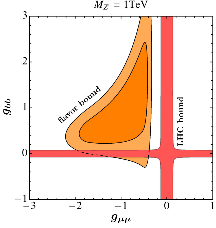 Figure 1
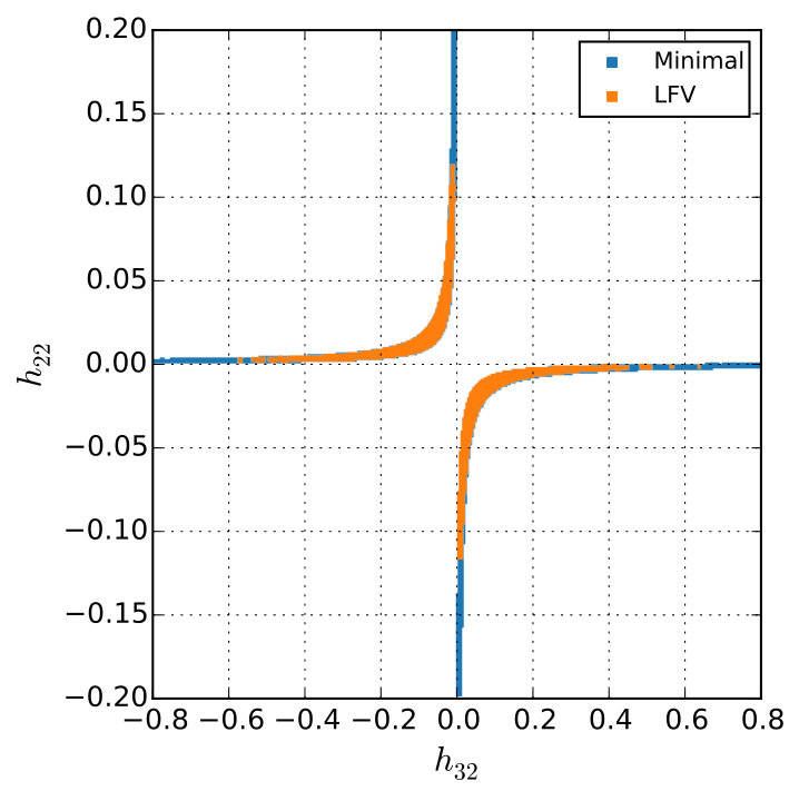 Figure 2
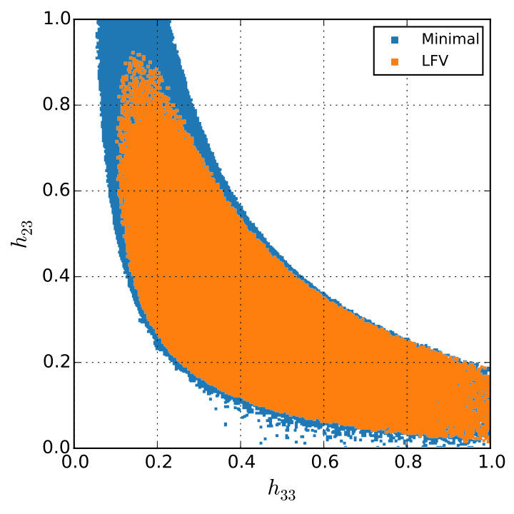 Figure 3
| Observable | Measurement or Constraint |
|---|---|
| minimal | |
| (all) | Alok:2017sui |
| RD_BaBar ; RD_Belle ; RD_LHCb ; Abdesselam:2016xqt | |
| RD_BaBar ; RD_Belle ; RD_LHCb ; Abdesselam:2016xqt | |
| Abdesselam:2017kjf | |
| Aaij:2017tyk | |
| Alok:2017jgr | |
| LFV | |
| ; (90% C.L.) Lees:2012zz | |
| ; (90% C.L.) Lees:2012zz | |
| ; (90% C.L.) Lees:2010jk | |
| (90% C.L.) Miyazaki:2011xe | |
| (90% C.L.) Ablikim:2004nn |
Peer Reviews
No public reviews on file for this paper yet. If you reviewed it on a platform where reviews are public (OpenReview, ICLR, NeurIPS, ICML), you can paste yours below so the community can read it here.
Videos
No videos yet. Explain this paper in a talk, walkthrough, or lecture? Add one.
Taxonomy
TopicsParticle physics theoretical and experimental studies · Computational Physics and Python Applications · Dark Matter and Cosmic Phenomena
Combined explanation of the B-anomalies
Jacky Kumar
Physique des Particules, Universit´e de Montr´eal, C.P. 6128, succ. centre-ville, Montr´eal, QC, Canada H3C 3J7
Abstract
There are four models of tree-level new physics (NP) that can potentially explain the and anomalies simultaneously. They are the S3, U3, and U1 leptoquarks and a standard-model-like triplet vector boson (VB). In this talk, I describe an analysis of these models with general couplings. We find that even in this most general case S3 and U3 are excluded. For the U1 model, I discuss the importance of the constraints from lepton- flavor-violating(LFV) processes. As for the VB model, it is shown to be excluded by the additional tree level constraints and LHC bounds on high-mass resonant dimuon pairs. This conclusion is reached without any assumptions about the NP couplings.
Currently, there are a number of measurements of the B-decays which do not agree with the standard model(SM). The size discrepancies vary from - and the combined significance based on the global fits amounts roughly to -. Here is the list of individual anomalies:
- •
In data, the measurements of the angular observables in and branching ratios in the decay deviate from the SM at the level of BK*mumuLHCb1 ; BK*mumuLHCb2 ; BK*mumuBelle ; BK*mumuATLAS ; BK*mumuCMS ; BsphimumuLHCb1 ; BsphimumuLHCb2 .
- •
The letpton flavor universality (LFU) ratios and which are defined to be ratio of the branching fractions for and modes in and decays respectively. Both are measured to be below the SM by about RKexpt ; RK*expt .
- •
The LFU ratios in the charge current decay , so called and , deviate from SM at the level of RD_BaBar ; RD_Belle ; RD_LHCb ; Abdesselam:2016xqt . Moreover, the also disagrees with the SM by about Aaij:2017tyk .
In terms of the individual explanations of neutral and charged current anomalies, the best way is to use weak effective theory(WET), which is valid below the electroweak weak scale. The effective lagrangian containing dimension six terms reads
[TABLE]
here , the wilson-coefficients(WCs) receive contributions from SM and NP. As far as transitions are concerned a shift in the WC of operators and is sufficient111Although after the Moriond 2019 update of measurementAaij:2019wad this picture has slightly changed.. For the charged current anomalies a NP contribution to the WC of operator is needed Capdevila:2017bsm ; Altmannshofer:2017yso ; DAmico:2017mtc ; Hiller:2017bzc ; Geng:2017svp ; Ciuchini:2017mik ; Celis:2017doq ; Alok:2017sui . For the combined explanation Standard model effective theory(SMEFT) is best suitable. The SMEFT is built from the operators upto dimension six made of the SM fields respecting the full SM gauge symmetryGrzadkowski:2010es . In SMEFT, the operator relates the to transitionsRKRD . Restricting ourselves to the (V-A) structure, we also need to consider operator which contribute to only to .
The next step is to look at the models which generate these two operators. Assuming that the SM is extended only by a single new particle, there are four possibilities. Three of them involve the Leptoquarks(LQs) and the fourth an addition vector boson. Three LQ models are scalar triplet(S3), vector triplet(U3) and vector singlet(U1). Here the transformation property refer to gauge group of SM.
Allowing the NP couplings to take general real values under the assumption that the NP couple only the second and third generations, a systematic analyses of these four models based on the paperKumar:2018kmr is presented here.
The Lagrangian of the LQ models read
[TABLE]
Each model can be described by four real couplings , here i and j can take values 2-3. The analysis is focused on the two things, first to find out which models work and second to analyze the pattern of the NP couplings for that purpose the LFV constrained turned out to be instrumental. The complete list of the observables playing an important role are shown in Table 1. The observables are divided into two categories which we refer as minimal constraints and LFV constraints.
First performing a fit using only the minimal constraints we establish which models work and then in the second step we add LFV constraints to figure out the pattern of the NP couplings.
The fit of S3 and U3 models to six minimal constraints gives and respectively. The degree of freedom(dof) in this case is two which is given by 6(No. of observables)- 4(No. of free parameters), implying a poor fit. The main reason for a bad fit is found to be the upper bound on the .
Moving to U1 model, in this case the transitions are forbidden at the tree level. Including LFV observables we have total 9 constraints and 5 dof. In this case is found at the best fit point, which means a good fit. Hence, U1 model is able provide a combined explanation to the both kind of anomalies. But the minimal observables constrain only the product of the couplings and . This is shown in the blue region of Figure 1.
Adding LFV constrains the allowed region as shown by the orange color. These constraints put the limits on the individual couplings as
[TABLE]
Furthermore, it was found that the LFV constraints prefer to be and a sizable Kumar:2018kmr . In the previous analyses( see e.g.CCO ; Bordone:2017anc ) a large coupling to the third generation was introduced as a theoretical assumption which turn out to be a requirement by the LFV constraints here.
Finally, the U1 model predicts
- •
the ratio
- •
for the ratio
- •
for the ratio
Coming to VB model, it involves six couplings and . An important difference from LQ models in this case is the presence of additional constraints due to -mixing and purely leptonic decays such as and at the tree level. It is found that -mixing and constrain . Because of this the NP effect on is very much limited and insufficient to accommodate anomalies. Therefore, the only option is to suppress the denominator of these observables which involve . But then the direct searches of heavy vector boson at the LHC in the channel CMS:2016abv turn out to be problematic. This is shown in Figure 2.
Therefore we conclude that:
- •
In case of leptoquarks, the S3 and U3 models are excluded by the constraint due to the upper bound on the . The U1 model with a large coupling to the third generation and a sizable provides the combined explanation of the B-anomalies and predicts a large enhancement in the .
- •
The VB model is excluded due to constraints coming from -mixing, -decays and direct searches in the dimuon channel at the LHC.
Acknowledgements.
It was a wonderful experience to be at FPCP 2019, I thank the organizers of the FPCP 2019 for that . I also thank to David London and Ryoutaro Watanabe for collaborating in this work. This work was financially supported in part by NSERC of Canada.
The reference list from the paper itself. Each links out to its DOI / PubMed record.
- 1(1) R. Aaij et al. [LH Cb Collaboration], Phys. Rev. Lett. 122 , no. 19, 191801 (2019) doi:10.1103/Phys Rev Lett.122.191801 [ar Xiv:1903.09252 [hep-ex]].
- 2(2) B. Grzadkowski, M. Iskrzynski, M. Misiak and J. Rosiek, JHEP 1010 , 085 (2010) doi:10.1007/JHEP 10(2010)085 [ar Xiv:1008.4884 [hep-ph]].
- 3(3) J. Kumar, D. London and R. Watanabe, Phys. Rev. D 99 , no. 1, 015007 (2019) doi:10.1103/Phys Rev D.99.015007 [ar Xiv:1806.07403 [hep-ph]].
- 4(4) R. Aaij et al. [LH Cb Collaboration], “Measurement of Form-Factor-Independent Observables in the Decay B 0 → K ∗ 0 μ + μ − → superscript 𝐵 0 superscript 𝐾 absent 0 superscript 𝜇 superscript 𝜇 B^{0}\to K^{*0}\mu^{+}\mu^{-} ,” Phys. Rev. Lett. 111 , 191801 (2013) doi:10.1103/Phys Rev Lett.111.191801 [ar Xiv:1308.1707 [hep-ex]].
- 5(5) R. Aaij et al. [LH Cb Collaboration], “Angular analysis of the B 0 → K ∗ 0 μ + μ − → superscript 𝐵 0 superscript 𝐾 absent 0 superscript 𝜇 superscript 𝜇 B^{0}\to K^{*0}\mu^{+}\mu^{-} decay using 3 fb -1 of integrated luminosity,” JHEP 1602 , 104 (2016) doi:10.1007/JHEP 02(2016)104 [ar Xiv:1512.04442 [hep-ex]].
- 6(6) A. Abdesselam et al. [Belle Collaboration], “Angular analysis of B 0 → K ∗ ( 892 ) 0 ℓ + ℓ − → superscript 𝐵 0 superscript 𝐾 ∗ superscript 892 0 superscript ℓ superscript ℓ B^{0}\to K^{\ast}(892)^{0}\ell^{+}\ell^{-} ,” ar Xiv:1604.04042 [hep-ex].
- 7(7) ATLAS Collaboration, “Angular analysis of B d 0 → K ∗ μ + μ − → superscript subscript 𝐵 𝑑 0 superscript 𝐾 superscript 𝜇 superscript 𝜇 B_{d}^{0}\to K^{*}\mu^{+}\mu^{-} decays in p p 𝑝 𝑝 pp collisions at s = 8 𝑠 8 \sqrt{s}=8 Te V with the ATLAS detector,” Tech. Rep. ATLAS-CONF-2017-023, CERN, Geneva, 2017.
- 8(8) CMS Collaboration, “Measurement of the P 1 subscript 𝑃 1 P_{1} and P 5 ′ subscript superscript 𝑃 ′ 5 P^{\prime}_{5} angular parameters of the decay B 0 → K ∗ 0 μ + μ − → superscript 𝐵 0 superscript 𝐾 absent 0 superscript 𝜇 superscript 𝜇 B^{0}\to K^{*0}\mu^{+}\mu^{-} in proton-proton collisions at s = 8 𝑠 8 \sqrt{s}=8 Te V,” Tech. Rep. CMS-PAS-BPH-15-008, CERN, Geneva, 2017.