Higher-order time-stepping schemes for fluid-structure interaction problems
Daniele Boffi, Lucia Gastaldi, Sebastian Wolf

TL;DR
This paper develops and analyzes second-order time-stepping schemes for fluid-structure interaction problems using a distributed Lagrange multiplier approach, demonstrating their stability and effectiveness through numerical tests.
Contribution
It introduces and studies second-order time integration schemes for fluid-structure interaction using a distributed Lagrange multiplier framework, with proven stability and validated numerical results.
Findings
The schemes are unconditionally stable under certain conditions.
Numerical tests confirm the theoretical stability results.
Second-order accuracy is achieved in fluid-structure interaction simulations.
Abstract
We consider a recently introduced formulation for fluid-structure interaction problems which makes use of a distributed Lagrange multiplier in the spirit of the fictitious domain method. In this paper we focus on time integration methods of second order based on backward differentiation formulae and on the Crank-Nicolson method. We show the stability properties of the resulting method; numerical tests confirm the theoretical results.
Click any figure to enlarge with its caption.
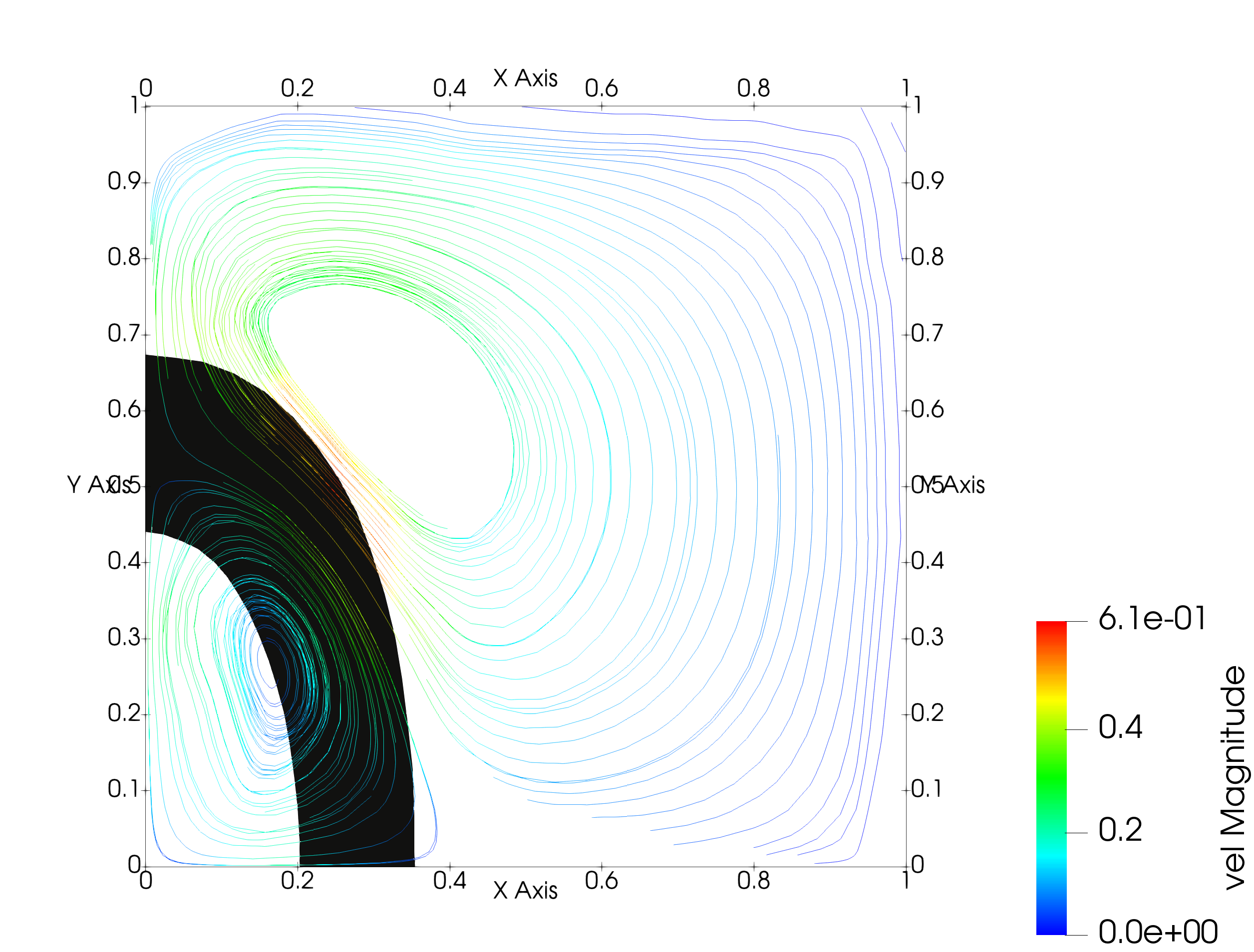 Figure 1
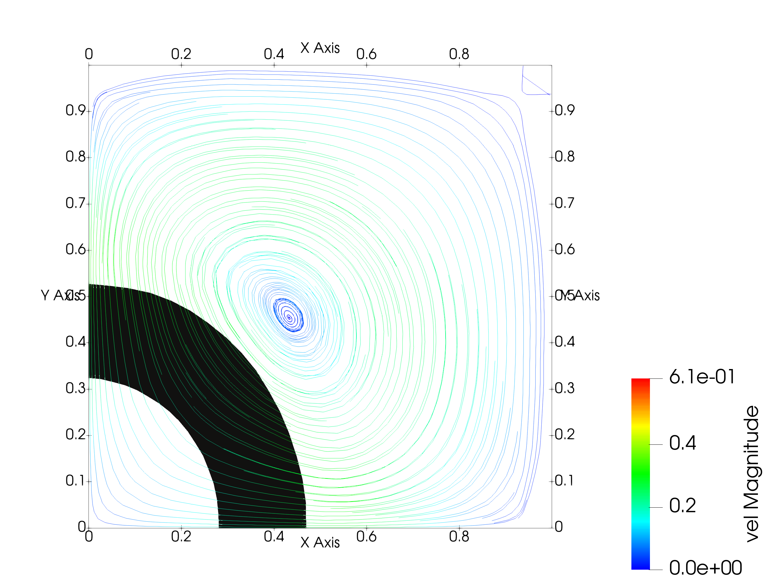 Figure 2
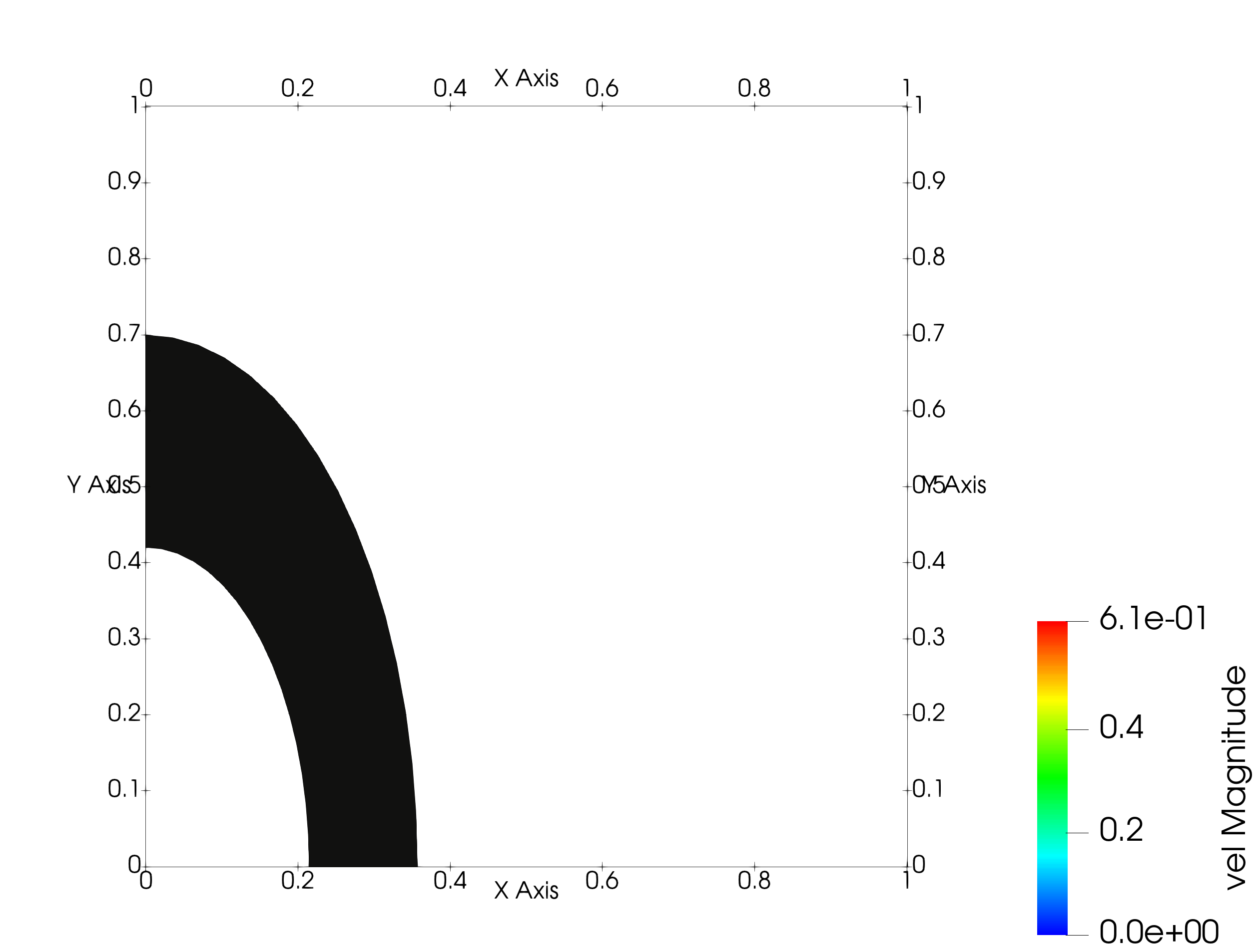 Figure 3
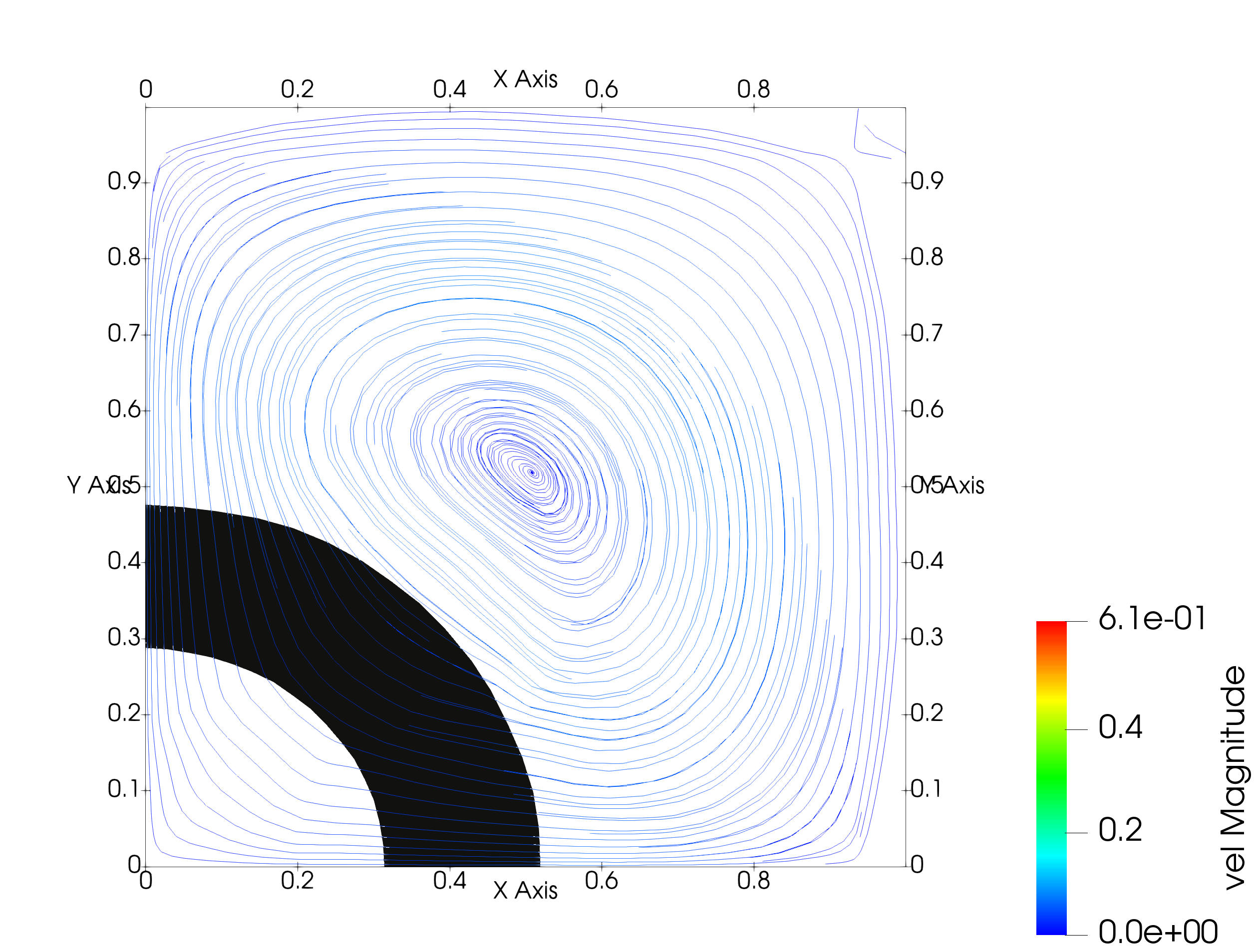 Figure 4
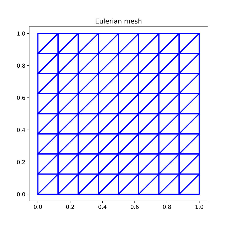 Figure 5
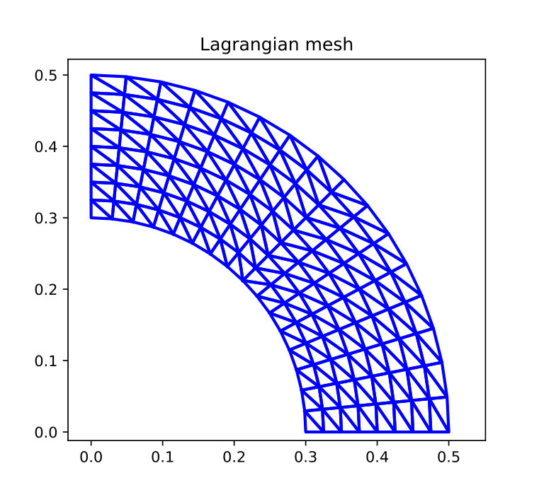 Figure 6
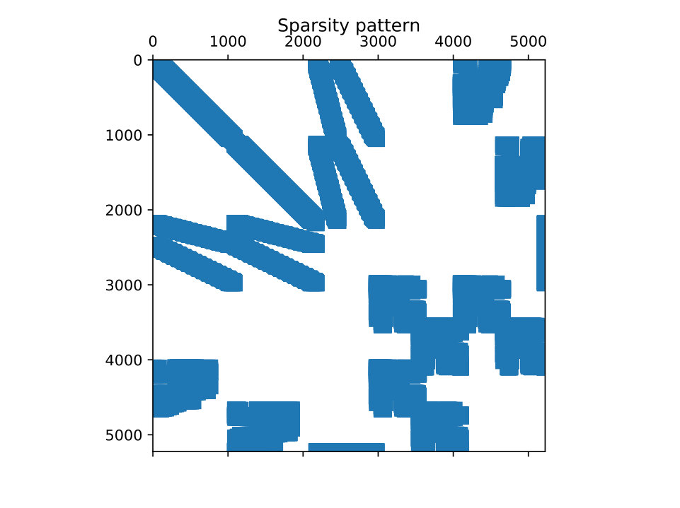 Figure 7
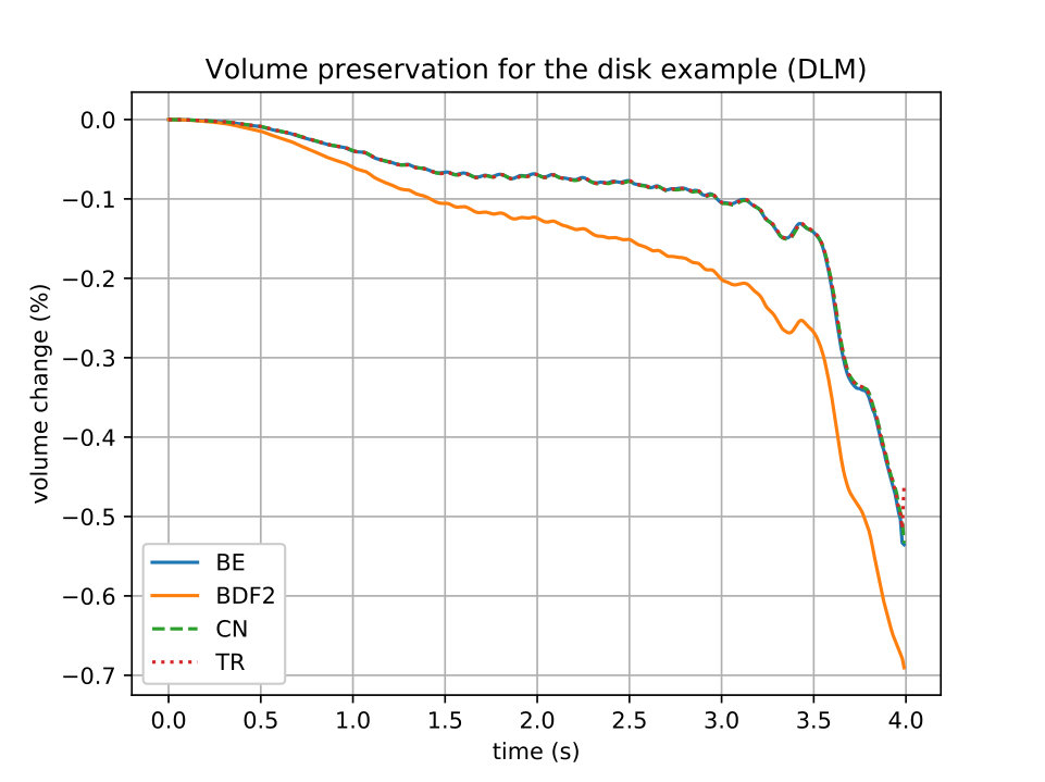 Figure 8
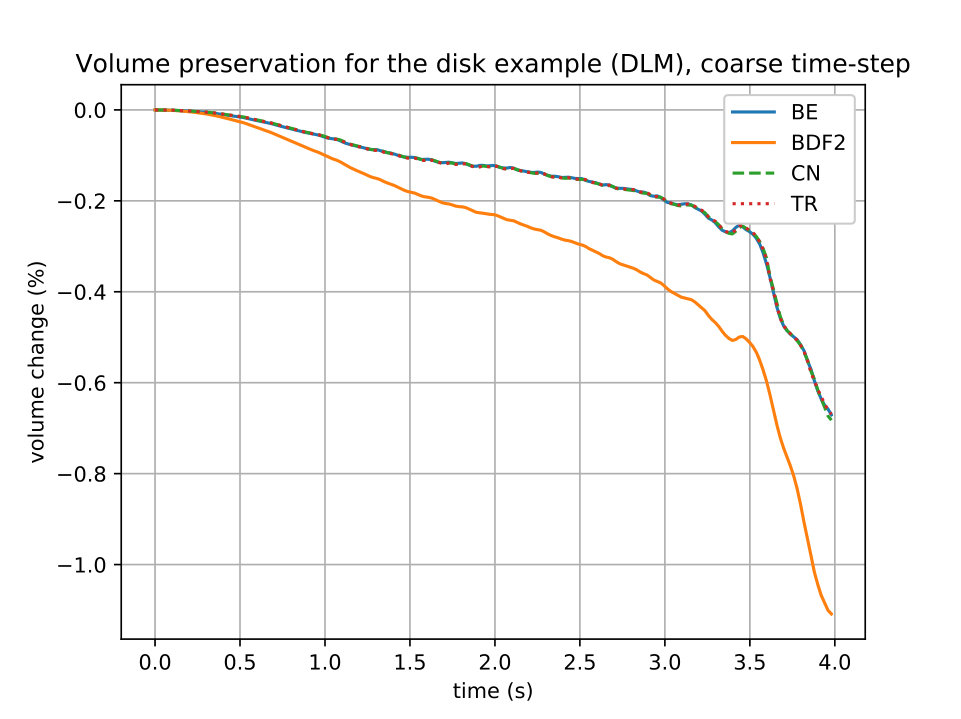 Figure 9
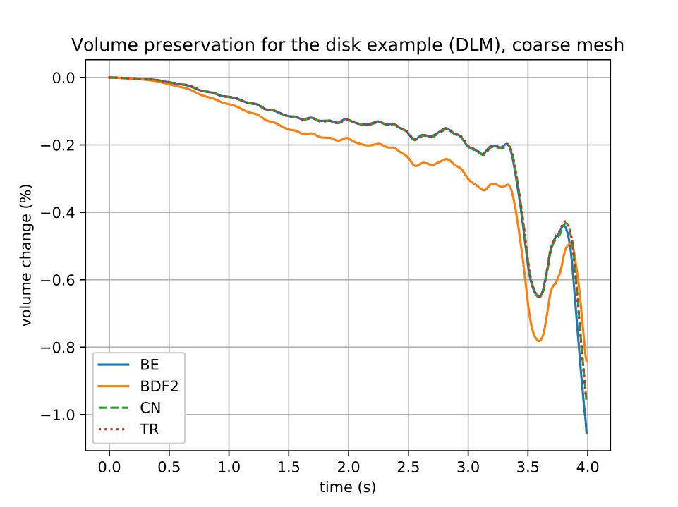 Figure 10
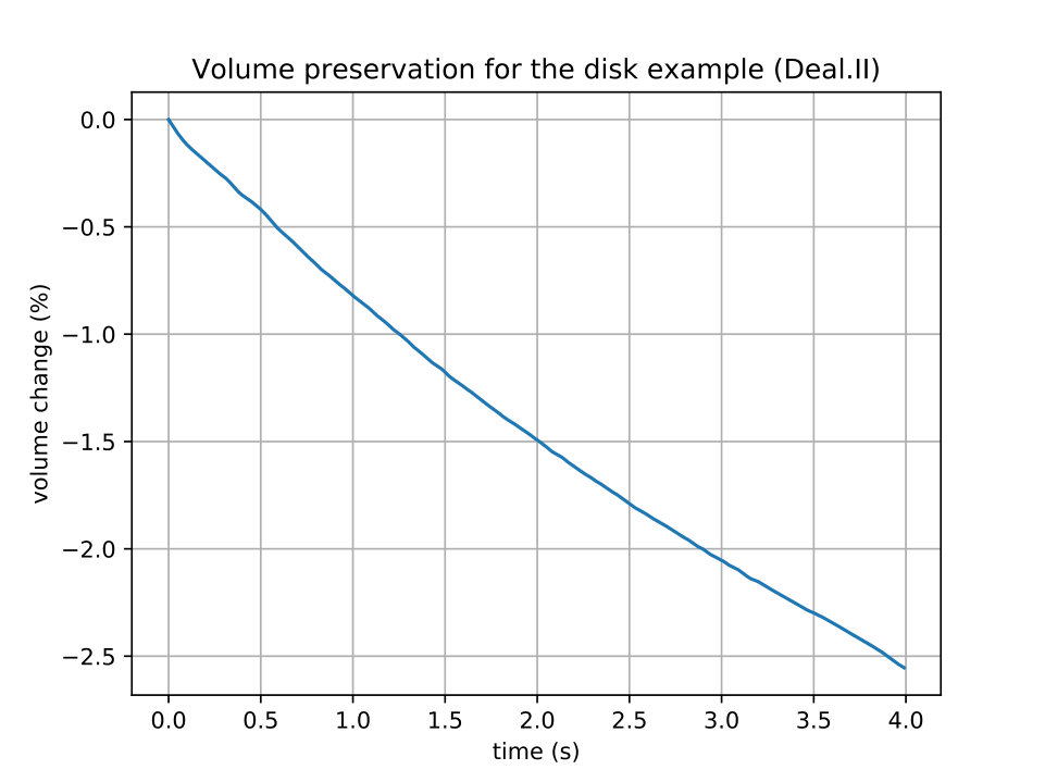 Figure 11
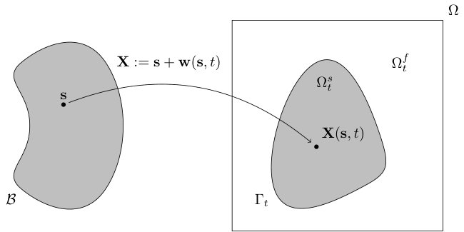 Figure 12
| DOFs | DOFs | DOFs | DOFs | |
|---|---|---|---|---|
| coarse mesh (M = ) | ||||
| fine mesh (M = ) |
| Fluid velocity | ||||||||
|---|---|---|---|---|---|---|---|---|
| BDF1 | BDF2 | CNm | CNt | |||||
| error | rate | error | rate | error | rate | error | rate | |
| Fluid velocity | ||||||||
|---|---|---|---|---|---|---|---|---|
| BDF1 | BDF2 | CNm | CNt | |||||
| error | rate | error | rate | error | rate | error | rate | |
| BDF1 | BDF2 | CNm | CNt | |
|---|---|---|---|---|
| BDF1 | BDF2 | CNm | CNt | |
|---|---|---|---|---|
| Fluid velocity | ||||||||
|---|---|---|---|---|---|---|---|---|
| BDF1 | BDF2 | CNm | CNt | |||||
| error | rate | error | rate | error | rate | error | rate | |
| Fluid velocity | ||||||||
|---|---|---|---|---|---|---|---|---|
| BDF1 | BDF2 | CNm | CNt | |||||
| error | rate | error | rate | error | rate | error | rate | |
| BDF1 | BDF2 | CNm | CNt | |
|---|---|---|---|---|
| BDF1 | BDF2 | CNm | CNt | |
|---|---|---|---|---|
Peer Reviews
No public reviews on file for this paper yet. If you reviewed it on a platform where reviews are public (OpenReview, ICLR, NeurIPS, ICML), you can paste yours below so the community can read it here.
Videos
No videos yet. Explain this paper in a talk, walkthrough, or lecture? Add one.
Higher-order time-stepping schemes for fluid-structure interaction problems
Abstract.
We consider a recently introduced formulation for fluid-structure interaction problems which makes use of a distributed Lagrange multiplier in the spirit of the fictitious domain method. In this paper we focus on time integration methods of second order based on backward differentiation formulae and on the Crank–Nicolson method. We show the stability properties of the resulting method; numerical tests confirm the theoretical results.
Key words and phrases:
Finite elements, Fluid-structure interactions, Fictitious domain, higher order time stepping, stability estimates
1991 Mathematics Subject Classification:
Primary: 65M60, 65M85; Secondary: 65M12, 74F10.
∗ Corresponding author: Daniele Boffi
Daniele Boffi∗
Dipartimento di Matematica “F. Casorati”, University of Pavia
Pavia, Italy
Lucia Gastaldi
DICATAM, University of Brescia
Brescia, Italy
Sebastian Wolf
Technische Universität München (TUM)
München, Germany
1. Introduction
We discuss a scheme involving a fictitious domain approach with a distributed Lagrange multiplier for the modeling of fluid-structure interaction problems [3, 5], which has originated as a natural evolution of the Finite Element Immersed Boundary Method introduced and studied in [6, 8, 2, 4]. This investigation started from the framework of Peskin’s research [19] who introduced the (finite difference) Immersed Boundary Method for the modeling of fluid-structure interaction problems.
The project described in this paper has been carried on during the Master thesis of the third author who spent a semester in Pavia within an exchange program between TUM and Pavia. The aim of the project was to investigate and analyze higher order time schemes for our fluid-structure interaction numerical approach which, so far, had been presented only in combination with low order Euler schemes. On the other hand, in the case of thick (codimension zero) solids, the regularity of the solution allows for a convergence in space higher than first order, so that it may pay off to make use of higher order schemes.
The main result of this paper consists in the implementation and in the stability analysis for the second order Backward Differentiation Formula BDF2 and for the Crank–Nicolson scheme. We present two possible variants of the Crank–Nicolson scheme, which differ in the treatment of the nonlinear terms.
The structure of our paper is as follows: after introducing the model and its finite element discretization in Section 2, we describe different time stepping schemes in Section 3: Backward Euler BDF1, BDF2, Crank–Nicolson (version based on midpoint rule CNm or based on trapezoidal rule CNt). Finally, in Section 4, we present several numerical experiments confirming the convergence and the stability proved in the previous section.
2. Setting of the FSI problem
We consider a fluid-structure interaction problem consisting of a visco-elastic solid immersed in a fluid. The solid is initially distorted from its equilibrium configuration, so that it tends to return to its equilibrium position. In doing so, the region occupied by the fluid changes its shape, thus inducing a flow which in turn produces a force on the solid, which deforms accordingly. We assume that both the fluid and the solid are incompressible. An extension to our model to compressible solids has been studied in [7] but is not going to be considered in this paper.
Let , with , be a connected, open, and bounded domain with Lipschitz continuous boundary . For simplicity, we assume that is a polyhedron. The domain is split into two non intersecting open domains and which represent the regions occupied at time by fluid and solid, respectively. Hence we have . We denote by the interface between and and assume that it has empty intersection with the exterior boundary . Let be the reference domain of , and let represent the corresponding deformation mapping. Hence a point is the image at time of a point , that is . For simplicity, we assume that is the initial position of the solid. We denote by the deformation gradient and by its Jacobian.
We are going to use the following notation: , , , and denote, respectively, velocity, pressure, stress tensor and density in the fluid. We consider a Newtonian fluid characterized by the usual Navier–Stokes stress tensor
[TABLE]
where is the fluid viscosity and . In the fluid, we use an Eulerian description so that the material derivative is given by
[TABLE]
In the solid, , , and stand, respectively, for velocity, pressure, and density. In the solid the Lagrangian framework is preferred, and the spatial description of the material velocity reads
[TABLE]
so that . Moreover, we assume that the solid material is viscous-hyperelastic, so that the Cauchy stress tensor is given by the sum of a viscous part
[TABLE]
where is the viscosity, and an elastic part , which can be expressed in terms of the Piola–Kirchhoff stress tensor :
[TABLE]
The Piola–Kirchhoff stress tensor is related to the positive energy density , which characterizes hyperelastic materials, as follows:
[TABLE]
where and . The elastic potential energy of the body is given by:
[TABLE]
Assuming that both the fluid and the solid material are incompressible, we have the following mathematical model for the fluid-structure system:
[TABLE]
The last two equations in (7) represent the transmission condition at the interface . The model is completed with initial and boundary conditions:
[TABLE]
Following [5], we apply a fictitious domain approach by extending the first equation in (7) to the whole domain and by using the following new unknowns:
[TABLE]
The extended velocity and pressure satisfy the following equation all over the domain:
[TABLE]
where we set
[TABLE]
The first equation in (10) enforces that in . By taking into account (2) and changing variable, this is equivalent to
[TABLE]
which subtracted from the third equation in (7) gives
[TABLE]
and the model problem can be rewritten as follows: find , , such that
[TABLE]
We observe that the second equation in (12) enforces the divergence free constraint both for fluid and solid. In order to arrive to our weak formulation we multiply the first equation by a test function and integrate by parts the right hand side taking into account (9) and the fact that the normal derivatives of might jump across , hence we have
[TABLE]
On the other hand, multiplying by a test function the third equation in (12) and integrating by parts, we obtain
[TABLE]
where is the outward normal unit vector to . By change of variables, the integral on the boundary is equal to the last integral on the right hand side of (13) if we choose for .
Let be a functional space to be defined later on and a continuous bilinear form such that
[TABLE]
Possible definitions for and are:
- •
is the duality pairing between its dual, that is and for , ;
- •
is the scalar product in , that is and for .
Then we introduce satisfying the following relation:
[TABLE]
Using the bilinear form we can formulate the kinematic constraint in the fourth equation in (12) as
[TABLE]
and our problem can be rewritten in the following weak form (see, also, [3, 5]).
Problem 1**.**
For given and , find , , , and such that for almost all :
[TABLE]
In the above problem we have used the following notation: , the scalar product in is denoted by , and
[TABLE]
Remark*.*
We remark that the unknown in Problem 1 plays the role of a Lagrange multiplier associated with the condition which enforces the kinematic constraint, that is the equality of the velocity with the solid velocity in the region occupied by the structures, see also (2).
Remark*.*
We can introduce an alternative to the third equation in (16) by splitting it into a system of two equations of first order in time, and by introducing a new unknown :
[TABLE]
This formulation is more suited when a second order time marching scheme is used, since we do not need to introduce a second order approximation of the second time derivative.
By choosing properly the test functions in (16), one can obtain the following energy estimate [5] :
Proposition 2.1*.*
Let us assume that , that the potential energy density is a convex function over the set of second order tensors, and that for almost every the solution of Problem 1 is such that with , then the following equality holds true
[TABLE]
In the above proposition stands for the norm in . We observe that the above proposition still holds true when the alternative formulation in (18) is used.
2.1. Finite element discretization
Let and be regular meshes in and , respectively, which are independent one from each other. The corresponding mesh sizes will be denoted by and , respectively. We consider two finite element spaces and such that the pair satisfies the usual inf-sup condition for the Stokes equations. We assume that contains only simplices and introduce the space of continuous piecewise affine functions on
[TABLE]
In order to discretize , we set . With this definition we have that when and is the duality pairing, we can compute easily using the scalar product in .
Then the discrete counterpart of Problem 1 reads as follows.
Problem 2**.**
For given and , find , , , such that for almost all :
[TABLE]
This semi discrete problem inherits the same energy estimate as the continuous one, which can be proved with the same technique.
The system (18) can be discretized as follows: find and such that
[TABLE]
We observe that the first equation can be solved exactly. In the following we shall use these two equations instead of the third equation in (21) when we apply higher order time marching schemes.
3. Higher-order time-stepping method
The system (21) is a system of ODEs with some algebraic constraints in , where . The numerical solution of Problem 2 can be computed by using some ODE/DAE solver. In order to avoid to use excessively small time steps, in [3, 5] the Backward Euler formula was applied for the time-integration, and the unconditional stability of the scheme has been proved. The aim of this paper is to introduce methods which achieve second order convergence in time and are unconditionally stable. In particular, we shall consider two one-step methods - based on the midpoint and trapezoidal rules - and the BDF2 method and analyze their stability. We observe that the resulting fully discrete scheme is nonlinear, and we shall discuss how the solution can be obtained.
3.1. Backward Euler
Before entering into the details of higher order methods, we recall the Backward Euler method analyzed in [3]. We subdivide the time interval into equal parts with size and subdivision points . Moreover, for a certain function , we set and use the following finite difference in order to approximate the time derivatives:
[TABLE]
Notice that both approximations are of first order.
The fully discrete version of Problem 1 using the Backward Euler scheme is the following one.
Problem 3**.**
Given and , for all find , , , and fulfilling:
[TABLE]
We recall the stability estimate proven in [3].
Proposition 3.1*.*
Let the material behavior be governed by an energy density which is and convex. Let and , be solutions of (24). Then the following estimate holds true:
[TABLE]
This system is highly nonlinear and hence not immediate to solve. It can be solved by a fixed-point method or by replacing some quantities at time with their known value at time . For example, in [3] the latter approach has been preferred; the value of in the first equation has been replaced by and, similarly, by . Moreover, as it is usual in the discretization of the Navier–Stokes equations, the first argument in the trilinear form has been evaluated at time . Notice that the same stability estimate as for the fully implicit scheme has been proved. We observe also that this modification introduces an approximation of first order, which should not affect the accuracy of the Backward Euler scheme, since it is of first order, too.
At the first step , the approximation of the second time derivative requires the knowledge of . Following [5], we can compute this value using the kinematic constraint and the initial data
[TABLE]
3.2. BDF2 method
Backwards differentiation formulae (BDF) are popular multistep methods to solve stiff ODE problems. They can be derived by approximating the time derivative at time with finite differences with order greater than or equal to 1. In particular, using a first order finite difference we have the Backward Euler method. In this paper we focus on the second order formula BDF2, hence, for a certain function , we approximate the time derivative with
[TABLE]
When applied to ODEs, it is well-known that BDF2 is convergent of order 2 and A-stable, (see for more detail [10, Chapter 7]). BDF methods have been successfully applied to the Navier–Stokes equations [16], to nonlinear structural mechanics [11], to electro-magnetic problems [18], and to Stokes–Darcy flow [9].
The application of the BDF2 method to Problem 2 gives the following formulation.
Problem 4**.**
Given , , for all find , , , and fulfilling:
[TABLE]
To start the computations, we additionally need the quantities and which are usually obtained by a one-step method. To achieve second order consistency theoretically, we need to apply a method of second order to the first step. This can be done, for instance, by using the Crank–Nicolson scheme, which is analyzed in this paper as well. In our numerical experiments we also tried a start-up with the backward Euler method, which also produced second order convergence.
In the following proposition, we prove an energy estimate for the scheme described by Equations (26a)-(26f).
Proposition 3.2*.*
Assume that and that the solids behavior is linear: . Let , , , be solutions of Problem 4, then the following estimate holds true:
[TABLE]
Proof.
We mimic the proof of [3, Prop. 3] and use some useful tricks presented in [16]. We test (26a) with :
[TABLE]
We remind that the trilinear form vanishes when the last two arguments coincide. The third term reduces to . Then by testing (26b) with , we see that the divergence term vanishes. Applying the following formula to the first term
[TABLE]
with , , , we obtain
[TABLE]
We are now left with the treatment of the term involving . We take in (26e) and in (26d), and use (26c) to obtain:
[TABLE]
Using the formula (28) we have
[TABLE]
Similarly we bound the term involving the Piola–Kirchhoff stress-tensor using again (28):
[TABLE]
Putting all these relations together yields the result and concludes our proof. ∎
Summing up in (27) and dropping out positive terms, yields the following unconditional stability bound:
[TABLE]
We note that the scheme presented in (26a)-(26f) is a fully implicit system which involves the solution of a nonlinear equation, stemming from the convection part in the Navier-Stokes equation as well as from the kinematic coupling term. The problem can be presented in the following matrix form:
[TABLE]
with
[TABLE]
Here , , , and denote the basis functions in , , , and , respectively.
Thanks to the theory developed in [5], we know that the linearization of the system above is associated to a steady saddle point problem which admits a unique solution. Moreover, the finite element discretization is stable, thus giving optimal convergence rates depending on the regularity of the solution.
We can either solve this system by a solver for nonlinear systems of equations like a fixed point iteration or Newton like methods, or make this semi-implicit by replacing the implicit terms with explicit ones. In the numerical experiments reported in the last section, we used a fixed point iteration or the well known extrapolation formula , in order to replace by and by .
3.3. Crank–Nicolson scheme
The Crank–Nicolson scheme is another second order method widely used for the discretization of evolutionary equations thanks to the fact that it is A-stable and one-step. In the literature, we can find two different schemes referred to as Crank–Nicolson scheme, which can be obtained by applying either the midpoint (CNm) or the trapezoidal (CNt) rule to integrate the ODE from to . Notice that the two methods coincide when the problem is linear. As far as the Navier–Stokes equations are concerned, in [15] the CNm approach is used and the stability properties are analyzed, while the CNt formula has been introduced, for example, in [17, Chapter 7]. We are going to apply both formulations in order to compare their numerical performances.
Let us start with the CNm version of the method.
Problem 5**.**
Given and , for all find , , , , and such that
[TABLE]
Equation (30e) is obtained by applying the midpoint rule to the kinematic constraint. Hence we approximate the value and we average both and providing an approximation which is second order accurate. The following proposition states a stability estimate similar to the one for the BDF2 method.
Proposition 3.3*.*
Assume and that the material behavior is governed by an energy density which is and convex. Let and , for , be the solutions of Problem 5. Then the following estimate holds true:
[TABLE]
Proof.
We mimic again the proof of [3, Prop. 3]. We take in (30a) to get:
[TABLE]
The trilinear form vanishes since the second two arguments coincide. Equation (30b) implies that the terms including the divergence vanish. If the initial condition is discretely divergence free, the theorem even hold for . Hence the above equality reduces to
[TABLE]
We set in (30e), then, using the equations in the solid (30c) with and (30d) with , we arrive at
[TABLE]
Now we want to see how the last term relates to the energy (6). Let us define the function by
[TABLE]
The convexity of is inherited from , so we see . Using the chain rule, we obtain . This is exactly the integrand in the term we want estimate. We obtain
[TABLE]
Putting all equations together yields the result. ∎
Again we can sum the equations with respect to from [math] to and get the unconditional stability bound:
[TABLE]
If we use the CNt method, we are led to consider the problem:
Problem 6**.**
Given and , for all find , , , and , such that:
[TABLE]
We omit the stability analysis of this problem which is not straightforward not even for the Navier–Stokes equations. Nevertheless this scheme has been used in our numerical tests and instabilities seem not to occur.
Both Problems (5) and (6) can be presented in matrix form with the a structure similar to that of BDF2, with some terms properly modified. The solution of the resulting nonlinear system can be obtained with a Newton like solver, Picard iterations, or by linearization. In our numerical experiments we adopted the latter two approaches.
4. Numerical Experiments
In this section we present some numerical results, with the aim of verifying the accuracy of the higher-order schemes presented in the previous sections. We consider fluid and solid with the same density and same viscosity . In our numerical experiments we adopt either Picard iterations or the semi-implicit schemes obtained by linearization of the nonlinear terms with second order extrapolations. More precisely, we substitute the value of a certain quantity with .
The first test case is the deformed annulus considered in [3] where convergence tests illustrate the first order rate for the implicit Euler method. The second test case is the floating disk for which we want to analyze the volume conservation properties of our methods.
In all our experiments, we use triangular meshes both in and , enhanced Bercovier–Pironneau elements (i.e. iso/) for the discretization (see [1]) and elements for the discretization of the body’s deformation , body’s velocity and the distributed Lagrange multipliers . We evaluate the bilinear form by means of the scalar product.
At each time step or at each fixed point iteration we have to assemble the matrix in (29) and to solve the resulting algebraic system. First of all, we observe that the matrix is neither symmetric nor positive definite. The sparsity pattern of the matrix is shown in Fig. 2.
Another aspect that influences the computational time is the assembly of the coupling terms. In order to construct the contribution of the matrix , we have to integrate on an element in the Lagrangian mesh quantities living on the Eulerian mesh such as . Numerically, this is done using some quadrature formula on . Consequently, we have to find all intersecting elements of the fluid mesh such that . Essentially this results in checking every deformed solid element against each fluid element. Bounding boxes are a good tool to detect when two cells surely do not intersect. This reduces the computational cost for each cell to cell comparison. Anyway, the computational cost for finding the intersecting cells grows linearly with the number of cells:
[TABLE]
Although, the theoretical analysis allows to choose meshes for the fluid and the solid independently one from each other, it has been observed, for example in [14], that the mesh parameter of the solid should be approximately half the size of the mesh parameter of the fluid. This can be explained as a trade-off between accuracy and computational effort.
4.1. The deformed annulus
In this test, an annulus is placed at the center of a square filled with some fluid. Initially the annulus is deformed from its initial configuration and the fluid is at rest. The internal forces steer the annulus back into its undeformed configuration and set the surrounding fluid into motion. The material of the annulus is hyperelastic and described by the identity . Thanks to the symmetry of the geometry, we run the simulation in the upper right quarter of the domain. The fluid’s domain is the unit square . On the upper and right boundary we impose no-slip boundary conditions for the fluid velocity. The reference domain for the immersed structure is a section of the annulus: . On the remaining part of the boundary, the fluid and the solid are allowed to move along the tangential direction, while the normal component is set to [math]. The initial conditions are
[TABLE]
The meshes for the fluid and the structure are schematically reported in Fig. 3.
We use two meshes whose number of degrees of freedom can be found in Table 1.
In Fig. 1 we report the position of the annulus and the streamlines of the velocity corresponding to the following choice of parameters , , , . The BDF2 method is used with . The snapshots are taken at , , , and .
In what follows, we report some tests to investigate the higher-order convergence of the BDF2 method and the two version of the Crank–Nicolson scheme CNm and CNt and compare them with the backward Euler method BDF1. The convergence tests are done using the two meshes plotted in Fig. 3 and parameters , , , and . Solutions have been calculated for . Since in this case no analytic solution is available, for each mesh we computed a reference solution using the BDF2 method with time-step and we report the relative errors with respect to it. When we use Picard iterations to obtain the solution of fully implicit schemes, we calculate the residual in the -norm and stop the iteration when it is less than the tolerance .
We first investigate the convergence of the fully implicit scheme. The relative errors in the norm are displayed in Tables 2 and 3.
The backward Euler method shows a clean first order rate of convergence, while the BDF2 method gives a clean second order rate of convergence only on the coarse mesh and in the fine mesh for the fluid velocity. The results for the structure displacement are not very clear on the fine mesh. The second order rate of convergence is achieved only for larger value of the time step and deteriorates as the time step decreases. On the other hand, we see that in this case the error is about , which is likely close to the accuracy that our fine mesh can provide. The CNt method achieves second order convergence for fluid and structure on both meshes, while the CNm scheme provides a second order convergence only for the fluid velocity. In general, the CNt scheme seems to perform better from the point of view of the rate of convergence and of the size of the error.
In order to investigate the behavior of the nonlinear solver, we track the maximum number of Picard iterations needed to reach the given tolerance. The results can be found in Tables 4 and 5. We observe that smaller time steps give smaller number of iterates. This can be motivated by the fact that we use the solution at the previous time step as the initial value for the iteration, therefore for smaller time step it is closer to the value at the current time.
In the case of fluid structure interaction, not only the nonlinear convection term has to be assembled at each iteration, but also the one coupling fluid and structure. Therefore, the semi-implicit scheme is attractive as it requires the solution of only one big system at each time steps. Results for the convergence study of the semi-implicit versions of the methods can be found in Tables 6 and 7.
We see a similar behavior as the one given by Picard iterations. The backward Euler method gives a good first order convergence. The BDF2 method shows a higher convergence order, which slows down for smaller time-steps in the fluid domain, in particular it is almost first order for the structure deformation. The behavior of the CNm is not very clear, in fact only the error in the fluid velocity on the coarse mesh achieves second order convergence. The CNt method provides better results which seem to respect the second order of convergence both for fluid velocity and structure deformation independently of the mesh.
Tables 8 and 9 report the residual obtained with the semi-implicit scheme which is higher of two orders of magnitude than the tolerance prescribed in the fixed point iterations. However, this fact does not influence too much the size of the errors.
4.2. The floating disk
In [12] it is pointed out that the Immersed Boundary Method may show poor volume conservation properties. Roy, Heltai, and Costanzo in [20] have compared the volume preservation properties of their numerical method and propose it as a benchmark problem for fluid-structure interaction codes. In the following we investigate the volume preserving properties of the higher-order time-stepping schemes applied to a circular disk placed in a lid-driven cavity. The movement of the fluid induces a motion to the disk, which is being deformed and transported.
The computational domain is a square with unit length: . The disk has a diameter of and its center is initially placed at . We describe Dirichlet boundary conditions on the fluid velocity: on the left, right, and bottom part of the boundary no-slip boundary conditions are enforced; on the upper part the fluid is set to . The fluid and the solid have the same density . The viscosity is and the material behaves as with . The final time of the simulation is . For the space discretization the same code as in the previous test is used on finer meshes with DOFs for the fluid velocity and DOFs for the pressure. The dimension of the space is equal to . The maximal diameter is for fluid elements, and for structure cells.
The simulation has been run for all the four time marching schemes with a time-step of . At each time-step the volume of the immersed solid is calculated and compared to the volume of the non-deformed solid. The percentage of volume change is plotted over time in Fig. 5. Throughout the literature on Immersed Boundary Method this problem has been addressed. Griffith and Luo [13] use a combination of finite differences for the fluid part and finite elements for the structure part. They report a volume conservation, which is more or less equal to results reported here. Wang and Zhan [21] use finite element discretizations for fluid and solid, while the coupling is enforced via some interpolation function, which mimics the Dirac in the continuous problem. They report a much larger volume change than what we have found. Even their volume preserving scheme performs worse. In our numerical experiments, we note that the one step methods give better volume preservation, whereas BDF2 method tends to reduce more the volume of the immersed solid.
The BDF1, the CNm, and the CNt schemes produce the same volume preservation pattern. In the beginning the volume decreases, from to the volume almost stays constant. In the last part of the time interval, the volume decreases again faster. At the end the volume is decreased by . The BDF2 method produces the same pattern, but the volume change is larger, at the final time the volume is decreased by . It is interesting to note that the BDF2 method, which is more accurate than the Backward Euler, produces a bigger volume change.
To investigate further the influence of the discretization parameters , , and on the volume preservation, the equations have been solved again, once on the same fine mesh with the doubled time-step and once on a coarser mesh with the same time-step . The coarse mesh consists of velocity DOFs, pressure DOFs and DOFs for the structure deformation and the Lagrangian multiplier. The volume preservation is plotted over time in Fig. LABEL:VolumePreservationCoarse for the coarse mesh (left) and the coarser time-step (right). One can observe that the qualitative behavior is similar to that reported in Fig. 5 for the fine mesh and double time step . The behavior on the coarser mesh, reported in Fig. LABEL:VolumePreservationCoarse (left), presents a larger kink at the end of the interval with respect to that in Fig. 5 and the absolute volume change is approximately doubled, at the end the volume is decreased by .
We conclude that in absolute numbers the volume change is the same for both simulations with less accuracy. The spatial discretization has a bigger influence on the qualitative behavior than the time discretization. This results is perfectly compatible with the fact that the area loss is strictly related to the approximation of the divergence free condition which, in turn, depends on the spatial discretization.
With a maximal area change of on the fine mesh with the fine time-step our method performs very well in comparison to other methods. A direct comparison is done with the method developed by Heltai and Costanzo in [14]. Their approach is quite similar to ours. They use a finite element approximation in space based on rectangular meshes and Backward Euler method for the time discretization. Their solver has been run with velocity DOFs, pressure DOFs and DOFs for the displacement field. This resulted in a maximal volume change of . A plot over time is shown in Figure 7. It is interesting to note that the volume change is monotone for this method, while our method shows some oscillations. This could be due to the different type of meshes and the fact that intersection of a mapped structural element with the elements in the fluid mesh are simpler to detect.
5. Conclusion
In this paper we discussed a finite element discretization of fluid-structure interaction problems based in the use of a distributed Lagrange multiplier. We introduced three higher-order time-stepping methods: BDF2, CNm, and CNt. We have proved unconditional stability estimates and we have performed a series of numerical tests. In the numerical experiments the BDF2 and CNt methods showed-higher order convergence in the fully implicit version. Using a semi-implicit approach, the CNt method showed second order convergence.
Acknowledgments
The first and the second authors are members of the INdAM Research group GNCS and their research is partially supported by IMATI/CNR and by PRIN/MIUR
The reference list from the paper itself. Each links out to its DOI / PubMed record.
- 1[1] D. Boffi, N. Cavallini, F. Gardini, and L. Gastaldi. Local Mass Conservation of Stokes Finite Elements. J. Sci. Comput. , 52:383–400, 2012.
- 2[2] D. Boffi, N. Cavallini, and L. Gastaldi. Finite Element approach to Immersed Boundary Method with different fluid and solid densities. Math. Models Methods Appl. Sci , 21(12):2523–2550, 2011.
- 3[3] D. Boffi, N. Cavallini, and L. Gastaldi. The Finite Element Immersed Boundary Method with Distributed Lagrange Multiplier. SIAM J. Numer. Anal. , 53(6):2584–2604, 2015.
- 4[4] D. Boffi and L. Gastaldi. Discrete models for fluid-structure interactions: The Finite Element Immersed Boundary Method. Discrete Contin. Dyn. Syst., Ser. S , 9:89–107, 2016.
- 5[5] D. Boffi and L. Gastaldi. A Fictious Domain Approach with Distributed Lagrange Multipliers for Fluid-Structure Interactions. Numer. Math. , 135:711–732, 2017.
- 6[6] D. Boffi, L. Gastaldi, and L. Heltai. Numerical stability of The Finite Element Immersed Boundary Method. Mathematical Models and Methods in Applied Sciences , 17:1479–1505, 2007.
- 7[7] D. Boffi, L. Gastaldi, and L. Heltai. A distributed Lagrange formulation of the Finite Element Immersed Boundary Method for fluids interacting with compressible solids. In Boffi D., Pavarino L., Rozza G., Scacchi S., and Vergara C., editors, Mathematical and Numerical Modeling of the Cardiovascular System and Applications , volume 16 of SEMA SIMAI Springer Series . Springer, 2018.
- 8[8] D. Boffi, L. Gastaldi, L. Heltai, and C. S. Peskin. On the hyper-elastic formulation of the immersed boundary method. Comput. Methods Appl. Mech. Eng. , 197:2210–2231, 2008.