On the Sample Complexity of HGR Maximal Correlation Functions for Large Datasets
Shao-Lun Huang, Xiangxiang Xu

TL;DR
This paper analyzes the sample complexity of estimating HGR maximal correlation functions using the ACE algorithm on large datasets, providing theoretical bounds, optimal sampling strategies, and supporting simulations.
Contribution
It develops a mathematical framework for understanding learning errors and error exponents in estimating HGR functions, and proposes an optimal sampling strategy for semi-supervised learning.
Findings
Derived analytical expressions for error exponents.
Established upper bounds for sample complexity.
Proposed an optimal sampling strategy to maximize error exponents.
Abstract
The Hirschfeld-Gebelein-R\'{e}nyi (HGR) maximal correlation and the corresponding functions have been shown useful in many machine learning scenarios. In this paper, we study the sample complexity of estimating the HGR maximal correlation functions by the alternating conditional expectation (ACE) algorithm using training samples from large datasets. Specifically, we develop a mathematical framework to characterize the learning errors between the maximal correlation functions computed from the true distribution, and the functions estimated from the ACE algorithm. For both supervised and semi-supervised learning scenarios, we establish the analytical expressions for the error exponents of the learning errors. Furthermore, we demonstrate that for large datasets, the upper bounds for the sample complexity of learning the HGR maximal correlation functions by the ACE algorithm can be…
Click any figure to enlarge with its caption.
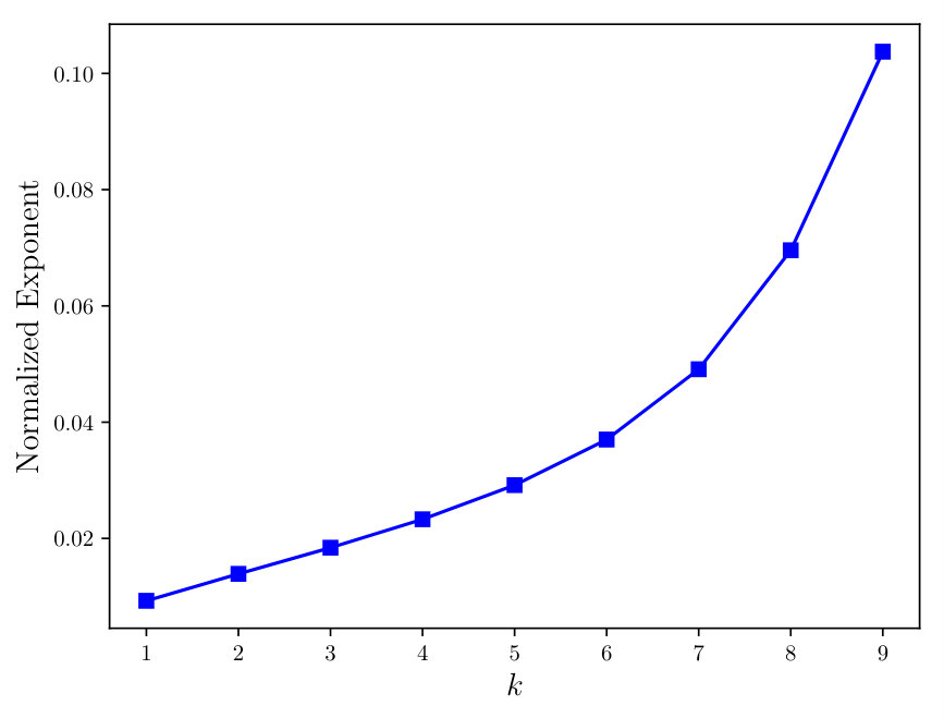 Figure 1
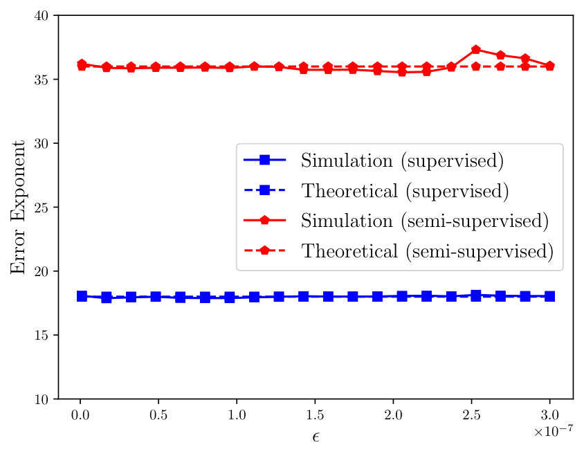 Figure 2
Peer Reviews
No public reviews on file for this paper yet. If you reviewed it on a platform where reviews are public (OpenReview, ICLR, NeurIPS, ICML), you can paste yours below so the community can read it here.
Videos
No videos yet. Explain this paper in a talk, walkthrough, or lecture? Add one.
On the Sample Complexity of HGR Maximal Correlation Functions for Large Datasets
Shao-Lun Huang, and Xiangxiang Xu This paper was presented in part at the Inform. Theory Workshop (ITW-2019), Visby, Sweden, Aug. 2019 and at Allerton Conf. Commun., Contr., Computing (Allerton-2019), Monticello, IL, Sep. 2019.S.-L. Huang is with the Data Science and Information Technology Research Center, Tsinghua–Berkeley Shenzhen Institute, Shenzhen, China (e-mail: [email protected]).X. Xu is with the Department of Electronic Engineering, Tsinghua University, Beijing, China (e-mail: [email protected]).
Abstract
The Hirschfeld–Gebelein–Rényi (HGR) maximal correlation and the corresponding functions have been shown useful in many machine learning scenarios. In this paper, we study the sample complexity of estimating the HGR maximal correlation functions by the alternating conditional expectation (ACE) algorithm using training samples from large datasets. Specifically, we develop a mathematical framework to characterize the learning errors between the maximal correlation functions computed from the true distribution, and the functions estimated from the ACE algorithm. For both supervised and semi-supervised learning scenarios, we establish the analytical expressions for the error exponents of the learning errors. Furthermore, we demonstrate that for large datasets, the upper bounds for the sample complexity of learning the HGR maximal correlation functions by the ACE algorithm can be expressed using the established error exponents. Moreover, with our theoretical results, we investigate the sampling strategy for different types of samples in semi-supervised learning with a total sampling budget constraint, and an optimal sampling strategy is developed to maximize the error exponent of the learning error. Finally, the numerical simulations are presented to support our theoretical results.
Index Terms:
error exponent, sample complexity, HGR maximal correlation, ACE algorithm, supervised learning, semi-supervised learning, singular value decomposition, generalization error
I Introduction
Learning informative and generalizable representations of data is a crucial issue in machine learning [1]. To measure the correlation and select informative features, the Hirschfeld–Gebelein–Rényi (HGR) maximal correlation [2, 3, 4] is a normalized measure of the dependence between two random variables and has been widely applied as an information metric to study inference and learning problems [5, 6, 7]. Specifically, given a pair of jointly distributed discrete random variables over finite alphabets , their HGR maximal correlation is defined as
[TABLE]
where the maximum is taken over all functions with zero mean and unit variance. Therefore, the HGR maximal correlation characterizes the correlation between the most correlated function mappings of and , and the optimal functions that achieve the maximal correlation essentially extract the most correlated aspects between and . Recently, the HGR maximal correlation has been further generalized to consider the correlation in the -dimensional functional spaces by defining [8]
[TABLE]
of which the special case with corresponds to the original problem (1). In particular, the optimal functions maximizing (2), referred to as the maximal correlation functions, have been shown to take important roles in statistics [6], information theory [8, 9], machine learning [10, 11, 12], and especially in interpreting deep neural networks [13]. For example, in machine learning scenarios, the variable can be viewed as the label, and is the data variable that is used to infer or predict about attributes of . Then, can be illustrated as the optimal feature to predict , with being the corresponding weights [12]. Therefore, efficiently and effectively computing maximal correlation functions from data is important in information theory and machine learning.
In this paper, we study the sample complexity of estimating the maximal correlation functions from a sequence of training samples , i.i.d. generated from the (unknown) true distribution , by the widely adopted alternating conditional expectation (ACE) algorithm [14]. Mathematically, the ACE algorithm computes the maximal correlation functions over the empirical joint distribution of the training samples. Therefore, there exists a learning error between the true maximal correlation functions and the computed functions due to the i.i.d. sampling process. To quantify this learning error, for functions computed from the ACE algorithm, we apply the H-score introduced by [13] as the performance metric. It has been shown that the H-score of a function indicates the performance of employing that function as the input feature to the softmax regression [13], and hence is a meaningful information metric in machine learning applications. Then, we study the large deviation property of the H-score for the functions computed from the ACE algorithm, in which we characterize the error exponent of the learning error in the asymptotic regime, i.e., when tends to infinity. In particular, we establish the analytical solutions for this error exponent expressed by the true distribution . Furthermore, for large datasets, we demonstrate an upper bound for the sample complexity of learning the maximal correlation functions, which can be expressed using the established error exponent. Our results also provide insights in designing the dimensionality for the selected features to effectively extract correlation structures among data variables in machine learning problems.
In addition, we investigate the sample complexity of the maximal correlation functions in the semi-supervised learning [15] scenario, in which not only the labeled samples, but also a sequence of unlabeled training samples is observed. In this case, the empirical joint distribution can in general be learned more accurately, since the marginal distribution of is trained better due to the unlabeled samples. Thus, the sample complexity is expected to be improved. To quantify this performance gain, we first propose a generalized ACE algorithm to deal with the unlabeled training samples, and then study the sample complexity of estimating the maximal correlation functions from the generalized ACE algorithm. As in the supervised case, we develop the closed form expressions for the error exponent of the learning error, and demonstrate the performance gain from the unlabeled samples. In addition, the theoretical results are applied to study the optimal sampling strategy, when the labeled and unlabeled samples have different acquiring costs. In particular, we formulate an optimization problem to maximize the error exponent of estimating the maximal correlation functions from different types of samples, subjected to a total budget constraint on acquiring these samples. The solution of this optimization problem then illustrates the optimal design of selecting different types of samples in semi-supervised learning problems. Finally, our theoretical results are supported by numerical simulations.
The rest of this paper is organized as follows. In Section II, we formulate the sample complexity problem of the maximal correlation functions and define the corresponding error exponent of the test error, and the mathematical framework for computing this error exponent is presented in Section III. In Section IV, we establish the analytical expression for the error exponent in the supervised learning scenario, in which the number of required samples for computing the maximal correlation functions on large datasets is provided. Then, similar analyses of the error exponent and the number of samples required for the semi-supervised learning are presented in Section V, in which we develop the optimal sampling strategy for semi-supervised learning with a sampling budget constraint. Finally, the numerical simulations are presented in Section VI to support our theoretical results.
II Problem Formulation
We commence by briefly introducing the singular value decomposition (SVD) structure of the HGR maximal correlation problem and the ACE algorithm for computing the maximal correlation functions. Given the joint distribution111We assume that the true marginal distributions , and , for all , since otherwise we can remove the symbols with probability 0 from the alphabets. , the HGR maximal correlation (1) is known to be the second largest singular value of the matrix , also referred to as the divergence transition matrix (DTM) [16], whose entries are [17]
[TABLE]
and the maximal correlation functions are chosen such that the vectors222In our development, we may simply take the alphabets and , which corresponds to some given alphabet orders of random variables and .
[TABLE]
are the right and left singular vector of associated with the second largest singular value, respectively. It can be shown that he largest singular value of is , with the corresponding right and left singular vectors being and , and thus it would be more convenient to subtract the top singular mode and introduce the matrix with entries
[TABLE]
referred to as the canonical dependence matrix (CDM) [18]. Then, the HGR maximal correlation and the 1-dimensional maximal correlation functions can be represented by the largest singular value and the corresponding singular vectors of the . It can be shown that the generalized HGR maximal correlation (2) has retained this SVD structure [18]. Specifically, the maximal correlation is the sum of the largest singular values (i.e., the Ky Fan -norm) of , and the maximal correlation functions correspond to its top right and left singular vectors, respectively.
In practical learning applications, since and can have large alphabets or even be continuous, the matrix cannot be easily estimated from data samples for computing the maximal correlation functions. Instead, we can use the ACE algorithm [14] to iteratively compute the maximal correlation functions, which is mathematically equivalent to the power method on . In particular, given a sequence of training samples , i.i.d. generated from the joint distribution , the ACE algorithm estimates the -dimensional maximal correlation functions of (2) can be summarized as Algorithm 1333There are also other variants of ACE algorithm for computing -dimensional maximal correlation functions using different numerical techniques for normalization, see, e.g., [8, Algorithm 3] and [18, Algorithm 1]., where the expectations are taken over the empirical distributions , or conditional distributions and from the training samples. In addition, and are the empirical covariance matrices defined as
[TABLE]
Now, let us define the and dimensional vectors and , respectively, for as
[TABLE]
where and are the empirical marginal distributions, and and are the -th dimension of and , i.e.,
[TABLE]
for all . In addition, we define as
[TABLE]
which is the CDM matrix for training samples. Then, the key steps of Algorithm 1 that alternatively compute conditional expectations (cf. line 4–6) can be equivalently expressed as alternating iterations [13, Eq. (10) and (12)]
[TABLE]
until stops increasing, where
[TABLE]
Note that (6) in fact coincides with the alternating least squares algorithm [19] for solving the low-rank approximation problem
[TABLE]
Therefore, from the Eckart–Young–Mirsky theorem [20], Algorithm 1 essentially computes the singular vectors of with respect to the top singular values, with more detailed illustrations provided in Appendix A for completeness. In the following, we simply use to denote the -th right singular vector of , and is the matrix formed by the top right singular vectors.
As discussed above, the maximal correlation functions of (2) correspond to the top singular vectors [cf. (4)] of the matrix as defined in (3). Therefore, if the empirical distribution coincides with the true distribution , then the matrix satisfies , and the ACE algorithm outputs the maximal correlation functions of (2) precisely. However, since the training samples are i.i.d. sampled from , the empirical distribution might deviate from the true distribution, which leads to deviations between the true singular vectors and the ones computed from the ACE algorithm. In order to quantify this deviation, we define the matrix as
[TABLE]
where is the -th right singular vector of . Then, we apply the difference of the Frobenius norm-squares as the measurement to quantify how deviates from . It is worth emphasizing that this measurement represents the test error of learned singular vectors and can be more effective than directly computing the difference between and . For example, consider the simplest case , and let denote the -th singular value of . Without loss of generality, we assume that the estimated satisfies , since if not we can use as the estimated singular vector. Then, it is shown in Appendix B that when , we have
[TABLE]
where the Frobenius norm becomes -norm since . Therefore, a small error in implies a small error measured in . However, when , both and (and thus any linear combination of and ) correspond to the maximal correlation function. While the measurement is able to indicate zero learning error for both optimal choices and , the measurement would indicate a large error for the optimal estimation .
In addition, this measurement can be interpreted as the performance of learning the matrix using by low-rank approximation, since
[TABLE]
Moreover, it is shown in [13] that is related to the softmax regression loss, and is called H-score therein, which provides the operational meaning for our selected performance measurement.
Note that , for all matrices satisfying , where is the identity matrix. In this paper, our goal is to characterize the sample complexity in learning maximal correlation functions for large datasets, i.e., the minimum number of samples required such that with high probability, the learning error is small [21]. To this end, we first consider the related error exponent defined as444Throughout, all logarithms are base , i.e., natural.
[TABLE]
where the probability is measured over the i.i.d. sampling process from . In particular, the first limit in (10) indicates the asymptotic regime of we are interested in, since in large datasets the number of i.i.d. samples can be sufficiently large. Then, the second limit of is naturally from that in this asymptotic regime, the empirical distribution converges to the true distribution with high probability, and thus the learning error is small with high probability; see, e.g., [22, Proposition 4.6] or [18, Proposition 47] for a more rigorous characterization.
In the remaining sections, we will show that these two limits facilitate the derivation of the analytical solution for the error exponent (10), and further use this exponent to provide the upper bounds for the sample complexity on large datasets, where the test error is small. In order to establish the analytical solution of (10), in the next section, we develop a mathematical framework for computing the learning error for the empirical distributions close to the true distribution .
III The Matrix Perturbation Analyses
Suppose that is a symmetric matrix with the eigenvectors and the eigenvalues . In addition, we denote
[TABLE]
as the matrix formed by the top eigenvectors of . Then, it follows that
[TABLE]
where denotes the trace of the matrix. Now, suppose that is a family of symmetric matrices parametrized by with , and is an analytic function of with the Taylor series expansion
[TABLE]
where is the first-order derivative of with respect to at . In addition, let be the matrix formed by the top eigenvectors of defined similarly to (11). Then, when , the following lemma characterizes the second-order Taylor series expansion of with respect to .
Lemma 1**.**
Suppose that , then
[TABLE]
where denotes the trace of the matrix.
Proof.
See Appendix C. ∎
Moreover, for the case , we apply the notation , and define the indices set , and the complement set . Furthermore, we define the matrix as the submatrix of composed of the columns of with indices in . Then, the following lemma establishes the second-order Taylor series expansion of for the case .
Lemma 2**.**
Suppose that , then
[TABLE]
where is the minimal element of , and
[TABLE]
where are the top eigenvectors of .
Proof.
See Appendix D. ∎
Note that since the Frobenius norm , the results we developed in this section essentially characterize the difference between and with respect to the perturbations on due to the difference between and . These results will be useful when we derive the error exponent (10) in the rest of this paper.
IV The Supervised Learning
Given training samples , i.i.d. generated from the joint distribution , in this section we develop the error exponent (10) and an upper bound for sample complexity for large datasets, in both cases and , where and are the -th and -th largest singular values of .
IV-A The Sample Complexity for the Case
To delineate our results, we need the following definitions. First, we define the quantity for the given , which will be useful in characterizing the error exponent (10).
Definition 1**.**
Given a joint distribution and , we define the matrix as
[TABLE]
where , and denotes the -th singular value555We define for , if . of . In addition, is an matrix, whose entry at the -th row and -th column is defined as
[TABLE]
where is the Kronecker delta, and
[TABLE]
where “” denotes the Kronecker product, and represents the -th right singular vector of . Then, is defined as the spectral norm of .
Then, the error exponent as defined in (10) can be established as follows, whose proof will later be provided.
Theorem 1**.**
If , then the error exponent as defined in (10) is
[TABLE]
Then, the following result illustrates that, for large datasets where the learning error is typically small, an upper bound of sample complexity can be established using the error exponent .
Theorem 2**.**
For given , there exist an absolute positive constant that depends only on , such that for all and , we have
[TABLE]
for all , where we have defined
[TABLE]
and where is as defined in Definition 1.
Proof.
See Appendix G. ∎
From Theorem 2, to guarantee that the error in learning maximal correlation functions is within some small with probability at least , it suffices to use samples.
Remark 1**.**
For comparison, an upper bound of sample complexity was provided in [22, Proposition 4.6] and [18, Proposition 47]. In particular, this upper bound is obtained via analyzing the concentration properties of , with the assumption that the true marginal distributions and have been known in advance. While our analysis does not rely on such assumptions, the resulting upper bound of sample complexity for large datasets can be significantly tighter.
When we are interested in learning the entire correlation structure between , i.e., , the following proposition establishes a simple closed form solution of the error exponent.
Proposition 1**.**
If , , and , then we have and
[TABLE]
Proof.
See Appendix H. ∎
We then introduce the proof of Theorem 1, which will make use of the perturbation analyses established in Section III. To begin, we first define the following sets of empirical distributions.
Definition 2**.**
For all , the set is defined as
[TABLE]
where corresponds to the top right singular vectors of , as defined in (5) and (7). Moreover, the set is defined as
[TABLE]
Furthermore, to characterize the empirical distributions , we denote the difference between and the true distribution as
[TABLE]
which induces a one-to-one correspondence666Note that since is finite, we have for each with . Therefore, we can obtain the distribution from , via
. We also define the matrices and , with entries at the -th row and -th column being and
[TABLE]
respectively. Then, using Lemma 1, the matrix estimated from data samples with the empirical distribution in can be represented in a perturbation form illustrated as follows.
Lemma 3**.**
For given , there exists a constant , such that for all and , we have and
[TABLE]
Proof.
See Appendix E. ∎
Moreover, the following lemma characterizes the I-projection of onto the set , which will be useful for characterizing the error exponent.
Lemma 4**.**
*For and as defined in Definition 2, we have777Given a distribution , we adopt the notation [23, p. 431]
where is a set of distributions.*
[TABLE]
Proof.
See Appendix F. ∎
Based on the above lemmas, Theorem 1 can be established as follows.
Proof of Theorem 1.
First, it follows from Sanov’s theorem [23] that
[TABLE]
where “” is the conventional dot-equal notation.888In particular, we use to denote
Therefore, the error exponent (16) can be expressed as
[TABLE]
From Lemma 4, there exists an such that, for all ,
[TABLE]
In addition, note that from (20), for all we have D\bigl{(}\hat{P}_{XY}\big{\|}P_{XY}\bigr{)}>\frac{\epsilon}{\alpha_{k}}. Hence, for all we have
[TABLE]
which implies that
[TABLE]
Combining (26) and (27), we obtain (16). ∎
IV-B The Sample Complexity for the Case
The idea of deriving the sample complexity in this case is similar to the case . To delineate the result, we first define
[TABLE]
Similar to and defined in Section IV-A, for the case we define the matrix and to characterize the error exponent .
Definition 3**.**
Given , the matrix is defined as
[TABLE]
where and are as defined in (13)–(14), where , and are defined as, for all , {\bm{\vartheta}}_{ij}\triangleq\bm{\phi}_{j}\otimes\bigl{(}\tilde{\mathbf{B}}\bm{\varphi}_{i}\bigr{)}+\bm{\varphi}_{i}\otimes\bigl{(}\tilde{\mathbf{B}}\bm{\phi}_{j}\bigr{)}, where are defined as
[TABLE]
where are the top eigenvectors of the matrix , and is as defined in (22). In addition, is defined as the optimal value of the optimization problem999Here, we apply the vectorization operation to stack all columns of a matrix into a vector. Specifically, for , is a -dimensional column vector with the -th entry being .
[TABLE]
Then, the following theorem characterizes the error exponent for the general case where and can be equal, and the corresponding upper bound of sample complexity can be established similar to Theorem 2.
Theorem 3**.**
If , the error exponent as defined in (10) is
[TABLE]
Proof.
See Appendix I. ∎
Note that in (29) is dependent on , since is dependent on . Therefore, unlike Theorem 1, the optimal value of (127) is not simply the largest singular value of some given matrix, and the optimization problem (127) is in general neither convex nor concave. However, note that if is fixed, the optimization problem (127) is reduced to solving the largest singular value of . Therefore, we can first fix to compute (or update) , and then solve the largest singular vector of to update , and so forth. This iterative procedure, summarized in Algorithm 2, solves the local optimum of the optimization problem (127). In particular, to update (cf. line 13–16 of Algorithm 2), we project onto the eigenspace of associated with its largest singular value, where a learning rate is used to enhance the robustness of the update.
While there is in general no closed form solution for (127), for some special joint distributions the closed form solutions exist.
Corollary 1**.**
Suppose , and the joint distribution takes the form
[TABLE]
where the probabilities and satisfy and . Then for any dimension , we have and thus
[TABLE]
where
[TABLE]
are the none-zero singular values of the corresponding .
Proof.
See Appendix J. ∎
IV-C Remarks on the General Trend of Error Exponent
In machine learning problems, it is also interesting to investigate \bigl{\|}\tilde{\mathbf{B}}\hat{{\mathbb{\Phi}}}_{k}\bigr{\|}_{\mathrm{F}}^{2}/\bigl{\|}\tilde{\mathbf{B}}{\mathbb{\Phi}}_{k}\bigr{\|}_{\mathrm{F}}^{2}, which tells how effective is, compared to . In particular, this is studied by the asymptotic problem
[TABLE]
where are the top singular values of .
The error exponent (34) combining with Theorem 2 offers insights on designing the dimensionality to effectively extract the correlation structure among different data variables from a given set of training samples. In particular, since both and are discrete, the true distribution can be approximated by the empirical distribution of training samples, and then the normalized error exponent can be obtained via computing the corresponding or from .
However, in real algorithm designs, it is more useful to provide a general trend for error exponent over different . For certain symmetric joint distributions, it can be verified that the normalized error exponent is linear to . For example, consider the joint distribution as constructed in Corollary 1, then we have . However, one can easily construct examples that the error exponent is not monotonic with respect to , and the behavior is generally complicated.
To gain more insights, we uniformly sample101010In particular, we generate independent random numbers uniformly from for each entry of , and then normalize the sum of the entries to . the joint distribution from the distribution space of , and consider the empirical average of the error exponents (34) over the sampled joint distributions. Fig. 1 plots the empirical average of the error exponents over sampled joint distributions with and , from which we observe that the error exponent grows linear to , for small , and becomes super-linear when is large. Although we do not have a rigorous proof in this paper, this general trend of the normalized error exponent, combining with Theorem 2, may provide a practical design guidance for selecting the dimensionality of the maximal correlation functions in real problems.
V The Semi-supervised Learning
In the semi-supervised learning setup, in addition to the labeled samples , we also have unlabeled samples , where is the ratio between the labeled and unlabeled samples, and the unlabeled samples are assumed to be i.i.d. sampled from the marginal distribution and independent of the labeled samples. In order to estimate the maximal correlation functions from both the labeled and unlabeled samples, we denote the empirical distribution of the unlabeled samples as , and again apply and to denote the empirical joint and conditional distributions of the labeled samples. Moreover, we denote the empirical distribution for as , which is the empirical marginal distribution of over all samples, and can be expressed as
[TABLE]
Then, Algorithm 1 can be generalized to estimating the maximal correlation functions from both labeled and unlabeled samples. For this purpose, we define
[TABLE]
as the empirical joint distribution by including both the labeled and unlabeled samples, with the corresponding marginal distributions being and
[TABLE]
respectively. Similarly, we obtain the conditional distributions
[TABLE]
and
[TABLE]
Then, we can generalize Algorithm 1 to semi-supervised learning by replacing the all expectation operations taken over empirical distributions with the expectations taken over empirical distributions , respectively. In particular, let and denote the initially chosen functions of and , which are zero-mean over the distribution and , respectively. Then, the alternating conditional expectation operations (cf. line 13–16 of Algorithm 1) can be represented as:
[TABLE]
where and are the covariance matrices of and , defined as
[TABLE]
The idea of this generalization is that the unlabeled samples do not help the estimation of the conditional distribution , but improve the estimation of the marginal distribution . Therefore, the first step in the algorithm remains the same, while in the second step, the improved empirical marginal distribution is applied to improve the estimation of the conditional distribution . In practice, we may assume that the marginal distribution is much easier to estimate than the joint distribution [8], and hence the above generalized ACE algorithm can still be implemented for computing the maximal correlation functions from training samples. In this section, our goal is to characterize the corresponding error exponent for the generalized ACE algorithm (38) in the semi-supervised learning scenario.
To this end, let us define the matrix , with entries
[TABLE]
where is the marginal distribution of as defined in (37). Then, it is shown in Appendix K that the algorithm (38) essentially computes the top singular vectors of . In addition, we denote as the dimensional matrix with the -th column being the -th right singular vector of . Then for large datasets, the sample complexity of estimating the maximal correlation functions by the algorithm (38) can be characterized by investigating the error exponent
[TABLE]
where the probability is measured over i.i.d. samples from and the i.i.d samples from . In the following, we develop the error exponent (40) for the semi-supervised learning, for both cases and , where and are the -th and -th largest singular values of .
V-A The Sample Complexity for the Case
Similar to Section IV-A, we first define the matrix and the quantity , which will be useful in characterizing the exponent .
Definition 4**.**
For given , the matrix is defined as
[TABLE]
where is as defined in (13), and is an matrix with its entry at the -th row and -th column defined as
[TABLE]
for all and , where denotes the Kronecker delta. Then, is defined as the spectral norm of the matrix .
Then, the following theorem establishes the analytical form of the error exponent , whose proof will be later provided.
Theorem 4**.**
If , the error exponent as defined in (40) is
[TABLE]
Similar to the case of supervised learning, for semi-supervised learning we have the following result establishing the upper bound for the sample complexity of learning maximal correlation functions on large datasets.
Theorem 5**.**
For given and , there exists an absolute positive constant and that depends only on and , such that for all and , we have
[TABLE]
for all , where we have defined
[TABLE]
and where is as defined in Definition 4.
Proof.
See Appendix O. ∎
Furthermore, the performance gain of estimating the maximal correlation functions with the aids of the unlabeled samples can be characterized by the following proposition.
Proposition 2**.**
For all , the as defined in Definition 4 is a non-increasing and convex function of , and satisfies
[TABLE]
where is defined as111111The limit exists since is non-increasing and has a lower bound [math]. and we have with as defined in Definition 1.
Proof.
See Appendix P. ∎
From Proposition 2, the error exponent of semi-supervised learning is a non-decreasing function of . Thus, with more unlabeled data samples used to train maximal correlation functions, we can obtain better performance. Moreover, it follows immediately from the first inequality of (46) that
[TABLE]
where can be interpreted as the error exponent in the case where we replace all unlabeled data samples with labeled data samples and obtain labeled samples of . Therefore, the upper bound (47) simply implies that the labeled data is generally more useful in estimating the maximal correlation functions. However, this upper bound is achievable for certain cases, where the unlabeled data can be as useful as the labeled data, as illustrated in the following proposition (cf. Proposition 1).
Proposition 3**.**
If , , and , then we have , and thus
[TABLE]
Proof.
See Appendix Q. ∎
In Proposition 1 and Proposition 3, we are interested in learning the entire correlation structure between and , i.e., . In such cases, learning top singular vectors is equivalent to learning the last singular vector
[TABLE]
which depends only on the marginal distribution . Hence, the unlabeled data samples of is as useful as the labeled data samples of , and thus we can achieve the upper bound of (47).
We then introduce the proof of Theorem 1, which will again make use of the perturbation analyses established in Section III. To start, we define the sets of the joint distributions as follows.
Definition 5**.**
For all , the set is defined as
[TABLE]
where corresponds to the top right singular vectors of as defined in (39). Moreover, the set is defined as
[TABLE]
where for given and , the joint distribution is as defined in (36).
Furthermore, for each with the corresponding empirical distributions and , we introduce the one-to-one correspondences and , where is as defined in (21), and where, similarly, we have defined
[TABLE]
Moreover, we define as the -dimensional vector with the -th entry being , and define the matrix with the entries being
[TABLE]
where we have defined
[TABLE]
Then, similar to Lemma 3, the matrix estimated from data samples can also be represented in a perturbation form, as the following lemma expresses.
Lemma 5**.**
For given and , there exists a constant , such that for all and , we have and
[TABLE]
Proof.
See Appendix L. ∎
In addition, the following lemma characterizing the error exponent will be useful in our analysis, and can be obtained using Sanov’s theorem.
Lemma 6**.**
Given , we have
[TABLE]
where is as defined in (48).
Proof.
See Appendix M. ∎
From (54), for given , the error exponent is determined by the infimum of a weighted sum of K-L divergences. Furthermore, if we restrict our attention to the distributions , the following result provides a characterization of this infimum in the small regime, and will also be useful in our analysis.
Lemma 7**.**
For and as defined in Definition 5, we have
[TABLE]
Proof.
See Appendix N. ∎
Using Lemma 6 and Lemma 7, Theorem 4 can be established as follows.
Proof of Theorem 4.
From Lemma 6, the error exponent can be expressed as
[TABLE]
Moreover, from Lemma 7, there exists an such that for all , we have
[TABLE]
In addition, note that for all we have \left[D\bigl{(}\hat{P}_{XY}\big{\|}P_{XY}\bigr{)}+rD(Q_{X}\|P_{X})\right]>\frac{\epsilon}{\bar{\alpha}_{k}(r)}. Hence, for all we have
[TABLE]
which implies that
[TABLE]
Combining (56) and (57), we obtain (43). ∎
V-B The Sample Complexity for the Case
With , , and as defined in (28), we further introduce the quantity as follows.
Definition 6**.**
Given , , and , the matrix is defined as
[TABLE]
where and are as defined in (41)–(42), and is as defined in (14) and are defined as, for all , \bar{{\bm{\vartheta}}}_{ij}\triangleq\bm{\phi}_{j}\otimes\bigl{(}\tilde{\mathbf{B}}\bar{\bm{\varphi}}_{i}\bigr{)}+\bar{\bm{\varphi}}_{i}\otimes\bigl{(}\tilde{\mathbf{B}}\bm{\phi}_{j}\bigr{)}, where are defined as
[TABLE]
and where are the top eigenvectors of the matrix . Then, is defined as the optimal value of the optimization problem
[TABLE]
where is defined as
[TABLE]
Then we have the following result characterizing the error exponent (40), and the corresponding upper bound of sample complexity for large datasets can be established similar to Theorem 5.
Theorem 6**.**
If , the error exponent as defined in (40) is
[TABLE]
Proof.
See Appendix R. ∎
Note that in (58) is dependent on , since is dependent on . Therefore, unlike Theorem 4, the optimal value of (60) is not simply the largest singular value of some given matrix. However, if we fix , the optimization problem (60) is reduced to solving the largest singular value of . As a result, similar to the approach introduced in Section IV-B, we can alternatively solve the optimal and , as summarized in Algorithm 3.
Similar to Corollary 1, we can compute the sample complexity in closed form for some joint distributions.
Corollary 2**.**
For the joint distribution as constructed in Corollary 1, all non-zero singular values of the corresponding are as given by (33). Then, for all , we have , and thus the corresponding error exponent is
[TABLE]
Proof.
See Appendix S. ∎
V-C The Optimal Number of Samples with the Cost Constraint
In semi-supervised learning, while the labeled samples are more useful than the unlabeled samples in learning problems, it is often much more expensive to acquire the labeled samples than the unlabeled ones. Therefore, it is important to understand the fundamental tradeoff between the sampling cost and the performance in learning tasks. In the following, we investigate such tradeoff for the sample complexity of learning the maximal correlation functions.
Suppose that the costs of acquiring the labeled and unlabeled samples are and per sample, respectively, and the total budget for sampling is . Then, the number of labeled samples and the number of unlabeled samples we can get are constrained by . Without loss of generality, we consider the case , and it follows from Theorem 4 that the error exponent for estimating the -dimensional maximal correlation functions with these samples is , where . Hence, the optimal error exponent that can be achieved by the sampling budget is given by
[TABLE]
which immediately implies the following proposition.
Proposition 4**.**
Given the sampling budget constraint , the optimal number of labeled samples and unlabeled samples to optimize the sample complexity of estimating the -dimensional maximal correlation functions are
[TABLE]
where
[TABLE]
Note that the optimal ratio is independent of , which indicates the relative importance of the unlabeled samples compared to the labeled samples, by taking the sampling costs into account. While the optimization problem (63) has no analytical solution and is neither convex nor concave, we can solve the local optimum by the numerical differentiation approach [24]. In particular, the local optimum of can be computed via the updating rule
[TABLE]
where is the step size for computing the numerical differentiation, and is the learning rate for gradient descent.
VI The Numerical Simulations
In this section, we validate our theoretical results by some numerical simulations. In our experiments, we choose , and the joint distribution as
[TABLE]
In the following, we compare the empirical error exponents (10) and (40) for estimating dimensional maximal correlation functions with the theoretical results. Note that since the joint distribution of (64) is a special case of Corollary 1 and 2, we can apply the results from the corollaries as our theoretical benchmarks.
VI-A Supervised Learning
In this experiment, we sample the learning error as follows. For each sample of the learning error, we first generate pairs of , i.i.d. from , and then compute the from the empirical distribution of these pairs. Then, the singular vectors of are computed to get a sample of . We repeat this sampling process for the learning error for times, and consider the empirical probability
[TABLE]
over the samples. Then, the empirical error exponent can be computed as
[TABLE]
The comparison between the empirical error exponent and the error exponent computed from Corollary 1 is plotted in Fig. 2, in which we can see the coincidence between these two error exponents.
VI-B Semi-supervised Learning
In the experiment for the semi-supervised learning, for each sample of learning error, we take , and generate pairs of , i.i.d. from , and of , i.i.d. from , and then compute the according to the empirical distribution from (36). This sampling process for the learning error is repeated for times, and the empirical probability of the learning error exceeding is defined as
[TABLE]
Then, the empirical error exponent can be computed as
[TABLE]
The comparison between the empirical error exponent and the error exponent computed from Corollary 2 is plotted in Fig. 2, in which we can see the coincidence between these two error exponents.
Appendix A Alternating Conditional Expectation Algorithm (Algorithm 1)
For convenience, we assume that the empirical distribution and thus . Let denote the -th singular value of , we will show that Algorithm 1 converges to the maximal correlation functions and which achieve the maximal correlation .
To begin, let and be the matrix composed of top right singular vectors and left singular vectors of , respectively, as defined in Section II. Then, from the analyses in Section II, we know that after the alternating conditional expectation processes (cf. line 4–6 of Algorithm 1), and have the same column space. Then, after the whitening of in line 8, we have
[TABLE]
where is an orthogonal matrix. Then, with line 9–11, we obtain
[TABLE]
where (67) follows from the fact that , where . In addition, (68) follows from the fact that , and (70) follows from that since is orthogonal, with representing the identity matrix of order .
From (65) and (70), we know that
[TABLE]
Finally, we have
[TABLE]
As a consequence, and are the maximal correlation functions that achieve the HGR maximal correlation .
Appendix B Proof of Eq. (9)
Firstly, note that
[TABLE]
where the second equality follows from the fact that
[TABLE]
since form an orthonormal set. Therefore, we have
[TABLE]
where the second inequality follows from the assumption that . As a consequence, we obtain (9) as desired.
Appendix C Proof of Lemma 1
Suppose take distinct values, and the indices are defined such that and
[TABLE]
Therefore, we have
[TABLE]
where denotes the -th column of . We first consider the summation for ,
[TABLE]
where is composed of the first columns of . First, note that since is analytic, there exists a symmetric matrix such that
[TABLE]
In addition, the analyticity of implies that the eigenspace is also analytic [25], and thus has the expansion
[TABLE]
where , , and are matrices in . Moreover, the columns of form an orthonormal basis of the eigenspace of associated with , and thus . Then, from , we obtain
[TABLE]
which in turn implies
[TABLE]
where and are the identity matrix and the zero matrix in , respectively. Therefore, we have
[TABLE]
where the penultimate equality follows from the fact that , the last equality follows from (72), and is the identity matrix in .
In addition, we define the matrix
[TABLE]
where are the largest eigenvalues of . Then, it follows from the analyticity of that is analytic and can be written as
[TABLE]
where and are both diagonal matrices. Now, from we obtain
[TABLE]
Comparing the -order terms for both sides, we have
[TABLE]
and thus
[TABLE]
Left multiplying (74) by , we obtain
[TABLE]
where we have again exploited the fact that .
Now, we can rewrite of (73) as
[TABLE]
where (76a) follows from (74), and (76c) follows from (75). Furthermore, it follows from the eigen-decomposition of that
[TABLE]
where is the -th column of (). Similarly, we have
[TABLE]
Hence, we obtain
[TABLE]
and its Moore-Penrose inverse
[TABLE]
Therefore, we have
[TABLE]
and hence
[TABLE]
where to obtain (78b) we have used (74), and to obtain (78c) we have used the fact that is a zero matrix [cf. (77)], since is orthogonal to for all .
Then, from (73), (76) and (78), we obtain
[TABLE]
which implies that
[TABLE]
where (80a) follows from (77), and of (80c) is defined as . To obtain (80c), we have used the fact that both the columns of and form an orthonormal basis of the eigenspace of associated with the eigenvalue .
Moreover, similar to the above derivations, for any we have
[TABLE]
Then from (71) and (81), we have
[TABLE]
which finishes the proof of the lemma.
Appendix D Proof of Lemma 2
Suppose take distinct values, then we define indices such that and
[TABLE]
We first consider the case , which implies . From (79) we have
[TABLE]
which implies [cf. (80)]
[TABLE]
To obtain , note that
[TABLE]
where to obtain the third equality we have used the fact that , and to obtain the last equality used that is a zero matrix as a consequence of (72a).
Since the columns of are orthonormal vectors in the eigenspace of associated with the eigenvalue , we can write as , where satisfies . Moreover, from the definition of eigenvectors, is the matrix with orthonormal columns that maximizes
[TABLE]
Therefore, is the optimal solution of
[TABLE]
which implies that are the top eigenvectors of the matrix .
As a result, we have
[TABLE]
where , and are the top eigenvectors of the matrix .
Similarly, for , we have
[TABLE]
where is the minimal element of , and
[TABLE]
with being the top eigenvectors of . Therefore, we obtain
[TABLE]
where (83b) follows from Lemma 1.
Appendix E Proof of Lemma 3
First, let us define . Then for all , we have, using Pinsker’s inequality [26],
[TABLE]
Therefore, for all we obtain
[TABLE]
Thus, it follows from (22) that
[TABLE]
where the last inequality follows from (85) and the fact that . Hence, we have , where depends only on .
To prove (23), we first define for the convenience of presentation. From (21), we can represent the differences between the empirical marginal distributions and the true marginal distributions as
[TABLE]
where
[TABLE]
In addition, it follows from (87) and (88) that
[TABLE]
and
[TABLE]
Therefore, from (21) and (87)–(92) we have, for all ,
[TABLE]
which is equivalent to (23).
Appendix F Proof of Lemma 4
For and , we define the subset of as
[TABLE]
where denotes the -th right singular vector of , and is as defined in (22). Then, it is convenient to first establish the following useful lemma.
Lemma 8**.**
For all , we have
[TABLE]
Using Lemma 8, we establish Lemma 4 as follows. First, for all empirical distributions , it follows from Lemma 3 that
[TABLE]
From the perturbation analysis result of Lemma 1, we can represent the learning error as
[TABLE]
Therefore, for any , there exists an such that for all , we have
[TABLE]
This implies that
[TABLE]
From the first inequality of (99), we obtain
[TABLE]
As can be chosen to be arbitrarily close to [math], we must have
[TABLE]
It remains only to establish Lemma 8.
Proof of Lemma 8.
Since the set is closed, we have
[TABLE]
Then, for all with , it follows from (85) that is bounded for all . Hence, it follows from the second-order Taylor series expansion of the K-L divergence that
[TABLE]
Moreover, since and are probability distributions, it follows from (21) that
[TABLE]
Therefore, the characterization of (95) leads to the following optimization problem:
[TABLE]
As we will verify, although not imposed as a constraint, the condition can be satisfied for the optimal . Note that since both the objective function and the inequality constraint (104b) are quadratic, the optimal solution of (104) can be obtained via solving
[TABLE]
where we have interchanged the objective function and the quadratic function in the inequality constraint. Furthermore, we can show that (105) is equivalent to the optimization problem without the equality constraint, i.e,
[TABLE]
To see this, suppose that is the optimal solution of (106) with . Then, let , and we have
[TABLE]
which implies .
If , we have , and it follows from (22) that . Hence, we have , where is a -dimensional vector with its -th element being , and with the -th element being . Then, the objective function is zero since , which contradicts the assumption that is optimal. Moreover, if , then we can construct the matrix with elements . It can be verified that and the objective function in (105) for is times the corresponding value for . This again contradicts the optimality of . Therefore, we have , and the optimization problem (106) has the same solution as that of (105).
In addition, it can be shown that for such that , we must have , since otherwise we can set and rescale to , which increases the objective function of (106) due to (22). Therefore, the optimal solution satisfies the definition (21).
To simplify the objective function (106a), we employ the vectorization operation that stacks all columns of a matrix into a vector. Specifically, for , we use to denote the -dimensional column vector with the -th entry being . Then, we can rewrite (106a) as
[TABLE]
where to obtain (107b)–(107c) we have used the properties of trace that
[TABLE]
and to obtain (107d) we have used the fact that
[TABLE]
Moreover, it follows from (22) and (14) that . Thus, (107e) can be reduced to
[TABLE]
Since , the constraint of (106) is equivalent to . Therefore, the maximum of (108) is the largest singular value of , which is the optimal value of the objective functions in (106) and (105). This implies that the optimal solution of the original optimization problem (104) is , with the corresponding optimal value being . Let denote the corresponding optimal empirical distribution, then we have, for sufficiently small,
[TABLE]
where we have used the fact that .
Hence, we obtain and thus
[TABLE]
which implies (95).
∎
Appendix G Proof of Theorem 2
First, it follows from (27) that there exists an such that for all we have
[TABLE]
where we have defined .
Then, using Sanov’s theorem, we have for all ,
[TABLE]
where to obtain (112) we have used (110), to obtain (113) we have used the fact that , and to obtain (115) we have used the fact that .
Therefore, it suffices to choose such that
[TABLE]
which is equivalent to
[TABLE]
where we have used the fact that .
Appendix H Proof of Proposition 1
First, note that (13) can be reduced to
[TABLE]
where
[TABLE]
where is the -th left singular vector of . Then, from the facts that and , we know that is the only right singular vector associated with the singular value [math], and thus we have
[TABLE]
Then it follows from (14) that the -th entry of is
[TABLE]
where and denote the -th entry of and the -th entry of , respectively, and where to obtain (119a) we have exploited the fact that
[TABLE]
In addition, to obtain (119c), we have used the facts that
[TABLE]
and for ,
[TABLE]
where (121b) follows from the fact that the vector \Bigl{[}\sqrt{P_{Y}(1)},\dots,\sqrt{P_{Y}(|{\mathcal{Y}}|)}\Bigr{]}^{\mathrm{T}}\in\mathbb{R}^{|{\mathcal{Y}}|} is a left singular vector of the matrix associated with the singular value [math].
Hence, from (119) we have
[TABLE]
where is a block diagonal matrix defined as
[TABLE]
As a result, it follows from (117) that
[TABLE]
from which we can obtain the eigen-decomposition of . Indeed, since , we have . Therefore, from (123), the non-zero eigenvalues of are , with the corresponding eigenvectors . As a result, the largest eigenvalue (i.e., the largest singular value) of is
[TABLE]
where denotes the spectral norm of its argument.
Appendix I Proof of Theorem 3
The proof is similar to that of Theorem 1, except that we need to replace the perturbation analysis result of Lemma 1 with the corresponding result of Lemma 2. In particular, we extend the definition to the case via letting121212It can be verified that, we have if . Therefore, the definition (124) is a generalization of (20).
[TABLE]
Then, we define as the set of such that the corresponding from (21) satisfies
[TABLE]
where are as defined in (30). Then, analogous to Lemma 8, it is convenient to first establish the following result.
Lemma 9**.**
When , for all , we have
[TABLE]
Proof.
The proof is similar to that of Lemma 8. Using the second-order Taylor series expansion of the K-L divergence (102), the limit (126) can be characterized by the following optimization problem:
[TABLE]
Following the same argument as that for Lemma 8, the optimal solution of (127) can be obtained by solving
[TABLE]
where we have interchanged the objective function and the quadratic function in the inequality constraint, and removed the equality constraint.
Then, similar to (107), we can rewrite the objective function (128a) as
[TABLE]
where the second equality follows from the fact that . As a result, the optimization problem (128) can be rewritten as (31), and thus the optimal value is . Note that if , we may let for since it does not change the value of (128a). Then, it can be verified that the optimal value of (128) is , i.e., we have if .
Finally, using the same argument as that for Lemma 8, we conclude that the optimal value of (127) is and we have
[TABLE]
which implies (126). ∎
In addition, it follows from Lemma 2 and Lemma 3 that the corresponding learning error for the empirical distribution is
[TABLE]
Therefore, for any , there exists an such that for all , we have
[TABLE]
Then, using arguments similar to (99)–(101), we conclude
[TABLE]
Finally, following the same proof as that for Theorem 1, we obtain (32).
Appendix J Proof of Corollary 1
We first introduce two useful lemmas.
Lemma 10**.**
Suppose is as defined in Corollary 1 with the corresponding matrix as given by (3). Then, the matrix have singular values
[TABLE]
In addition, for all with
[TABLE]
the corresponding satisfies
[TABLE]
where denotes the vector in with all entries being .
Proof.
From the definition of , we have
[TABLE]
and
[TABLE]
Therefore, from (3) we have
[TABLE]
where is the zero matrix in . As a result, we have
[TABLE]
Since the matrix
[TABLE]
has eigenvalues and , we obtain the singular values of as given by (130), and thus we can rewrite (133) as
[TABLE]
Hence, for all with (131), we have
[TABLE]
where is the zero vector in . ∎
Lemma 11**.**
For all satisfying (131), we have
[TABLE]
where the inequality holds with equality if and only if , where
[TABLE]
Proof.
From we have
[TABLE]
Therefore, we obtain
[TABLE]
where the inequality follows from the fact that the arithmetic mean is no greater than the root mean square. As a result, we have
[TABLE]
where the inequality holds with equality if and only if
[TABLE]
Hence, it follows from (131) and (136) that . ∎
Now, Corollary 1 can be proved as follows.
Proof of Corollary 1.
From Lemma 10, we have . Therefore, for all we have , which further implies that and . Hence, from (29) we have
[TABLE]
In addition, following the same derivation as that in (119), we have
[TABLE]
and thus
[TABLE]
Note that since , (139) demonstrates the eigen-decomposition of . Therefore, from Theorem 3, we have
[TABLE]
To prove the inequality holds with equality, it suffices to show that there exists a with such that
[TABLE]
Indeed, as we now illustrate, if is chosen as
[TABLE]
with as defined in (135), then we have and , and thus (140) holds.
To see this, first note that from (141) we have ,
[TABLE]
and
[TABLE]
where .
Therefore, from (22) we obtain
[TABLE]
In addition, since , from (30), is the solution of the optimization problem
[TABLE]
where is the -th right singular vector of . Since and , we know that
[TABLE]
and thus is equivalent to .
Now, for all satisfying the constraints of (143), the objective function of (143) is
[TABLE]
where , and where to obtain (144c) we have used the fact that , to obtain (144d) we have used the facts that and , and to obtain (144e) we have used Lemma 10 and the facts that
[TABLE]
Furthermore, to maximize (144f), note that
[TABLE]
As a result, if follows from Lemma 11 that (144f) is maximized when , i.e., we have , which finishes the proof. ∎
Appendix K The Generalized ACE Algorithm (38)
First, we define the and dimensional vectors and , respectively, for as
[TABLE]
where and are the marginal distributions of , and and are the -th dimension of and , i.e.,
[TABLE]
for all and . Then, the iterative steps of the generalized ACE algorithm (38) can be equivalently expressed as
[TABLE]
where
[TABLE]
Note that (145) coincides with the alternating least squares algorithm [19] for solving the low-rank approximation problem
[TABLE]
Then, using the same argument as that in Appendix A, we know that the generalized ACE algorithm (38) essentially computes the singular vectors of with respect to the top singular values.
Appendix L Proof of Lemma 5
For any with the corresponding empirical distributions and , it follows from (49) that
[TABLE]
Then, following the same argument as that for (84), we obtain
[TABLE]
In addition, from (52) we have
[TABLE]
where to obtain the second inequality we have used the fact that .
Then, it follows from (86c) that
[TABLE]
Hence, we have with .
Turning now to the second part of the lemma, for the convenience of representation, in the following we use to replace .
From (35), (50) and (87), we conclude
[TABLE]
where and are as defined in (87) and (50). In addition, it follows from (21) and (87) that
[TABLE]
where is as defined in (21).
Therefore, we have
[TABLE]
Finally, it follows from (87)–(93) that
[TABLE]
Appendix M Proof of Lemma 6
First, note that
[TABLE]
where and denote the type class of and the type class of , respectively, and the last equality follows from the fact that is independent of . Then, the probabilities of the two type classes are [26]
[TABLE]
and
[TABLE]
Moreover, for both type classes, the numbers of types are at most polynomial in . Therefore, via the Laplace principle [27] it follows that
[TABLE]
Appendix N Proof of Lemma 7
For and , we define the subset of as
[TABLE]
where is as defined in (51). Then, it is convenient to first establish the following useful lemma.
Lemma 12**.**
For all , we have
[TABLE]
Using Lemma 12, we establish Lemma 7 as follows. First, for all , it follows from Lemma 5 that
[TABLE]
From the perturbation analysis result of Lemma 1, we can represent the learning error as
[TABLE]
Therefore, for any , there exists an such that for all , we have
[TABLE]
Then, using arguments similar to (99)–(101), from Lemma 12 we obtain
[TABLE]
It remains only to establish Lemma 12.
Proof of Lemma 12.
Since the set is closed, we have
[TABLE]
Then, for all with the corresponding empirical distributions and for labeled and unlabeled data, it follows from the second-order Taylor series expansion of the K-L divergence that
[TABLE]
Therefore, the characterization of the error exponent (40) can be reduced to the following optimization problem:
[TABLE]
where the equality constraints follow from the definitions of and . As we will verify, although not imposed as a constraint, the condition can be satisfied for the optimal . Since both the objective function and the inequality constraint of (155) are quadratic, the optimal solution can be obtained via solving
[TABLE]
where we have again interchanged the objective function and the quadratic function in the inequality constraint. Then, with arguments similar to those of the supervised case, we can verify the optimal solution of (156) also satisfies (21) and (52). Furthermore, it can be verified that (156) is equivalent to the optimization problem without the equality constraints, i.e.,
[TABLE]
To see this, suppose is the optimal solution of (157), and define and . With and , we have
[TABLE]
which implies .
If , then we have and , which implies and . Therefore, it follows from (51) that
[TABLE]
which implies that is a zero matrix. As a result, the objective function of (156) is zero, which contradicts the optimality of . Moreover, if , we can construct a feasible solution with
[TABLE]
and it is straightforward to verify that the objective function for is times the value for . This again contradicts the optimality of . Therefore, we have , and the optimization problem (157) has the same solution as (156).
To simplify the optimization problem (157), we define the vector as
[TABLE]
and let be the matrix with the entries . Then, it follows from (42) and (52) that .
Therefore, the objective function of (157) can be rewritten as
[TABLE]
where to obtain (160a) we have used (107), and to obtain (160c) we have used (13). In addition, since , the constraint of (157) can be rewritten as .
As a result, the maximum of (160e) is the spectrum norm of , i.e., , which is also the optimal value of the objective functions in (157) and (156). This implies that the optimal solution of the original optimization problem (155) is , with the corresponding optimal value being . Let and denote the corresponding empirical distributions, then we have, for sufficiently small,
[TABLE]
where to obtain the inequality we have used the fact that .
Hence, the corresponding optimal distribution as defined in (36) satisfies . Therefore, we conclude
[TABLE]
which implies (152).
∎
Appendix O Proof of Theorem 5
First, it follows from (57) that there exists an that depends only on and such that for all we have
[TABLE]
where we have defined .
Then, for all , it follows from (150) that
[TABLE]
where and denote the type class of and the type class of , respectively, and where (163) follows from the upper bound of probability of type classes [26, Theorem 11.1.4], where (165) follows from the upper bound of the number of types [26, Theorem 11.1.1]. In addition, (166) follows from (161), (167) follows from , (170) follows from the fact that , and (172) follows from the fact that since .
Therefore, it suffices to choose such that
[TABLE]
which is equivalent to
[TABLE]
where we have used the fact that .
Appendix P Proof of Proposition 2
First, we write the matrix as defined in (42) as , where is composed of the first columns of , and is composed of the rest columns of . Then it follows from the definition of that
[TABLE]
where is the identity matrix in , and is as defined in (122).
Therefore, we have
[TABLE]
where to obtain (174c) we have exploited the fact that is the identity matrix in .
Then, with denoting the spectral norm, we have
[TABLE]
where is defined as the positive semidefinite matrix such that , and where (175b) follows from the fact that for all matrices , we have
[TABLE]
Moreover, from we have
[TABLE]
where we have defined
[TABLE]
Then, it follows from (175c) and (176)–(177) that
[TABLE]
Furthermore, for all , we define as
[TABLE]
then it can be verified that satisfies \bigl{\|}\hat{\mathbf{P}}\bigr{\|}_{\mathrm{s}}=1 and . Hence, we have
[TABLE]
where the inequality follows from the submultiplicativity of the spectral norm [28].
To prove the convexity of , we first define the function for . Since is an increasing and concave function of , we have, for all and ,
[TABLE]
which implies that
[TABLE]
Therefore, we have
[TABLE]
where the first equality follows from the fact that is non-increasing, and the second equality follows from the triangle inequality for the spectral norm.
Finally, to obtain the lower bound of (46), note that
[TABLE]
where (178b) follows from the triangle inequality, (178c) follows from (176), (178d) follows from the submultiplicativity of the spectral norm, and the penultimate equality follows from the fact that , since is an identity matrix.
To obtain the upper bound of (46), note that
[TABLE]
where we have again used the triangle inequality.
Appendix Q Proof of Proposition 3
First, note that from (41) we have
[TABLE]
where the second equality follows from (123), and in the last equality we have defined
[TABLE]
In addition, note that satisfies
[TABLE]
where to obtain the second equality we have used (174c). Therefore, we have , and it follows from (179) that the non-zero eigenvalues of are
[TABLE]
Hence, the largest eigenvalue (i.e., the largest singular value) of is
[TABLE]
Appendix R Proof of Theorem 6
Similar to the proof of Theorem 3, we first extend the definition of to the case via letting
[TABLE]
and define as the set of such that the corresponding from (52) satisfies
[TABLE]
where are as defined in (59). Then the following result, analogous to Lemma 12 for the case , will be useful in our analysis.
Lemma 13**.**
For all , we have
[TABLE]
Proof.
The proof is similar to that of Lemma 9. Using the second-order Taylor series expansion of the K-L divergence (154), the limit (184) can be characterized by the following optimization problem:
[TABLE]
Following the same argument as that for Lemma 12, the optimal solution of (185) can be obtained by solving
[TABLE]
where we have interchanged the objective function and the quadratic function in the inequality constraint, and removed the equality constraints.
In addition, similar to (160), we can rewrite the objective function of (186) as
[TABLE]
where is as defined in (58). As a result, the optimization problem (186) can be rewritten as (60), and thus the optimal value is . Finally, using the same argument as that for Lemma 12, we conclude that the optimal value of (60) is and thus
[TABLE]
which implies (184). ∎
In addition, it follows from Lemma 2 and Lemma 5 that the corresponding learning error for the distribution is
[TABLE]
Therefore, for any , there exists an such that for all , we have
[TABLE]
Then, using arguments similar to (99)–(101), from Lemma 13 we have
[TABLE]
Finally, following the same proof as that for Theorem 4, we obtain (62).
Appendix S Proof of Corollary 2
From Lemma 10, we have . Therefore, for all we have , which further implies that
[TABLE]
Hence, from (58) we have
[TABLE]
In addition, similar to (119), we have
[TABLE]
and thus
[TABLE]
where is as defined in (180). Note that since , (190) demonstrates the eigen-decomposition of . Therefore, from Theorem 6 and the definition of , we have
[TABLE]
To prove that the inequality holds with equality, it suffices to construct and such that the corresponding as defined in (61) satisfies and
[TABLE]
Indeed, as we now illustrate, if and are chosen as
[TABLE]
with as defined in (135), then we have and , and thus (191) holds.
To see this, first note that from (173) we have
[TABLE]
and it follows from (61) and (192) that . Therefore, we have .
In addition, from (52) we have
[TABLE]
i.e.,
[TABLE]
Then, similar to (142), from (51) we obtain
[TABLE]
with as given by (142). Furthermore, following the same proof as that for Corollary 1, is the solution of the optimization problem
[TABLE]
which has the same solution as the optimization problem (143) since . Hence, we obtain , which finishes the proof.
The reference list from the paper itself. Each links out to its DOI / PubMed record.
- 1[1] Y. Bengio, A. Courville, and P. Vincent, “Representation learning: A review and new perspectives,” IEEE transactions on pattern analysis and machine intelligence , vol. 35, no. 8, pp. 1798–1828, 2013.
- 2[2] H. O. Hirschfeld, “A connection between correlation and contingency,” Proc. Cambridge Phil. Soc. , vol. 31, pp. 520–524, 1935.
- 3[3] H. Gebelein, “Das statistische problem der korrelation als variations-und eigenwertproblem und sein zusammenhang mit der ausgleichungsrechnung,” Z. für angewandte Math., Mech. , vol. 21, pp. 364–379, 1941.
- 4[4] A. Rényi, “On measures of dependence,” Acta Mathematica Academiae Scientiarum Hungarica , vol. 10, no. 3–4, pp. 441–451, 1959.
- 5[5] C. Bell, “Mutual information and maximal correlation as measures of dependence,” The Annals of Mathematical Statistics , pp. 587–595, 1962.
- 6[6] R. Ahlswede and P. Gács, “Spreading of sets in product spaces and hypercontraction of the markov operator,” The annals of probability , pp. 925–939, 1976.
- 7[7] D. Lopez-Paz, P. Hennig, and B. Schölkopf, “The randomized dependence coefficient,” in Advances in neural information processing systems , 2013, pp. 1–9.
- 8[8] A. Makur, F. Kozynski, S.-L. Huang, and L. Zheng, “An efficient algorithm for information decomposition and extraction,” in Communication, Control, and Computing (Allerton), 2015 53rd Annual Allerton Conference on . IEEE, 2015, pp. 972–979.