A multiscale reduced basis method for Schr\"{o}dinger equation with multiscale and random potentials
Jingrun Chen, Dingjiong Ma, Zhiwen Zhang

TL;DR
This paper introduces a multiscale reduced basis method for the semiclassical Schrödinger equation with multiscale and random potentials, effectively addressing high-frequency oscillations and enabling efficient numerical simulations in complex quantum systems.
Contribution
The paper develops a novel multiscale reduced basis approach combining optimization, proper orthogonal decomposition, and quasi-Monte Carlo methods for efficient Schrödinger equation solutions.
Findings
Method reduces spatial grid size proportional to the semiclassical parameter
Number of random samples inversely proportional to the semiclassical parameter
Numerical results confirm efficiency and accuracy of the approach
Abstract
The semiclassical Schr\"{o}dinger equation with multiscale and random potentials often appears when studying electron dynamics in heterogeneous quantum systems. As time evolves, the wavefunction develops high-frequency oscillations in both the physical space and the random space, which poses severe challenges for numerical methods. In this paper, we propose a multiscale reduced basis method, where we construct multiscale reduced basis functions using an optimization method and the proper orthogonal decomposition method in the physical space and employ the quasi-Monte Carlo method in the random space. Our method is verified to be efficient: the spatial gridsize is only proportional to the semiclassical parameter and the number of samples in the random space is inversely proportional to the same parameter. Several theoretical aspects of the proposed method, including how to determine the…
Click any figure to enlarge with its caption.
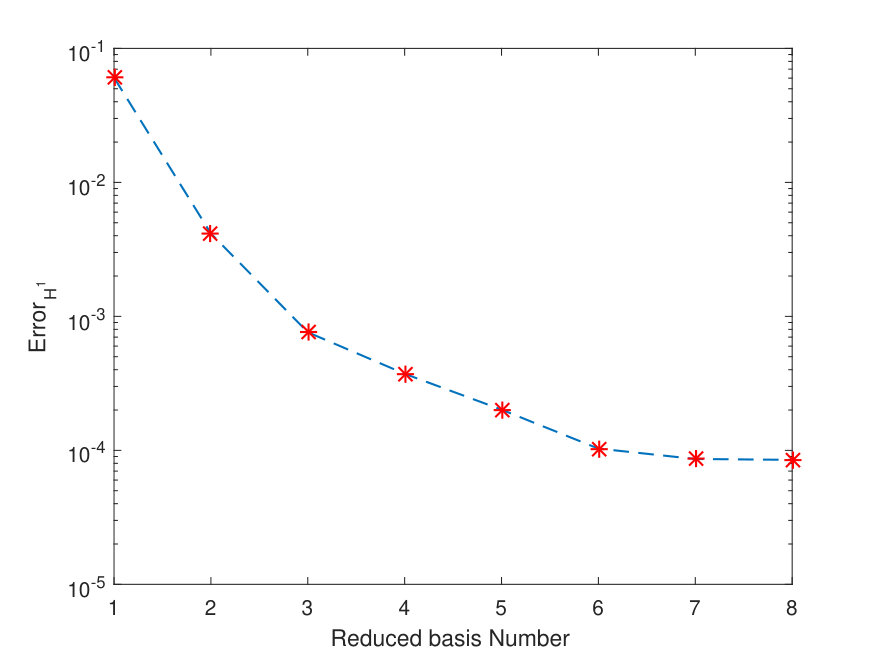 Figure 1
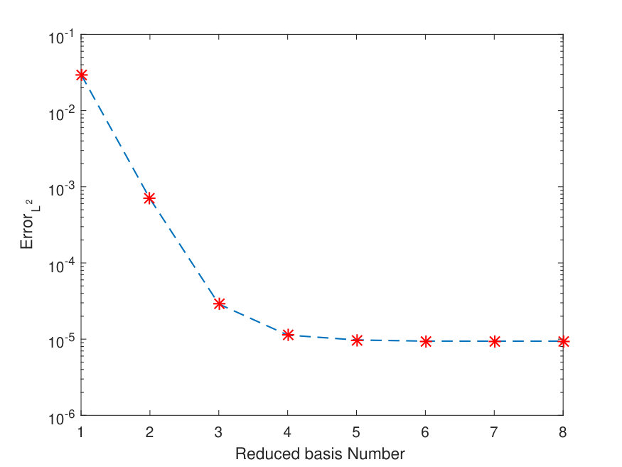 Figure 2
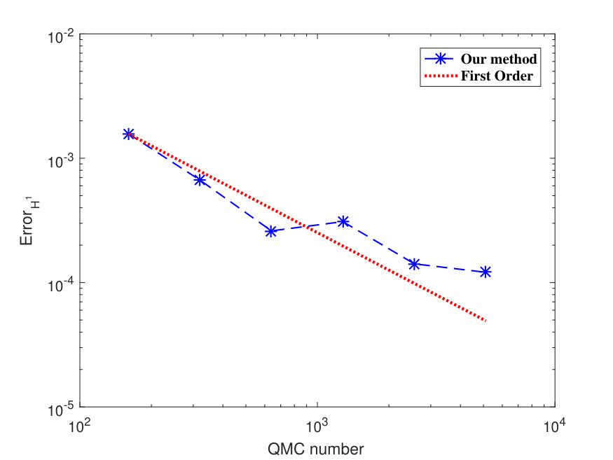 Figure 3
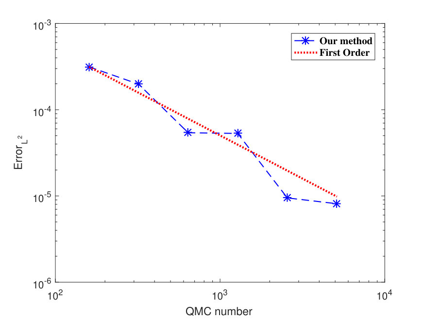 Figure 4
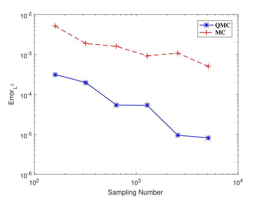 Figure 5
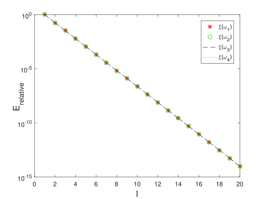 Figure 6
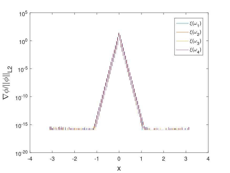 Figure 7
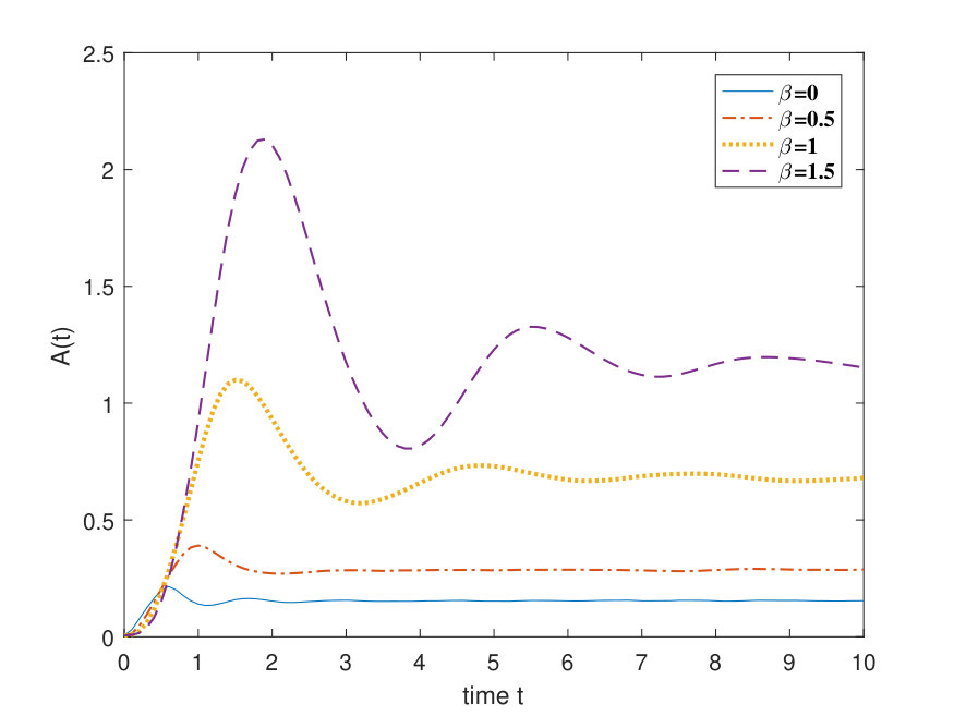 Figure 8
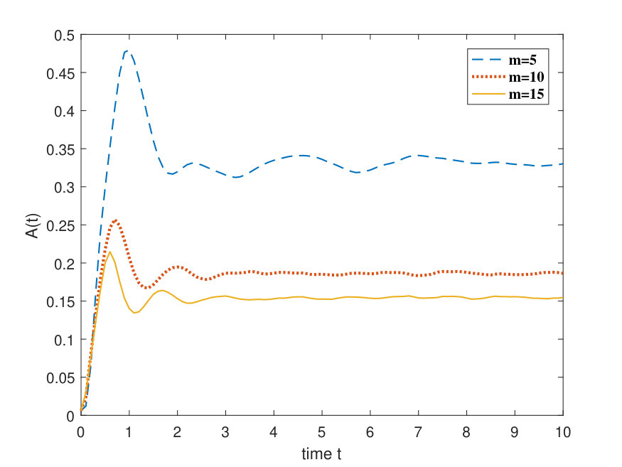 Figure 9
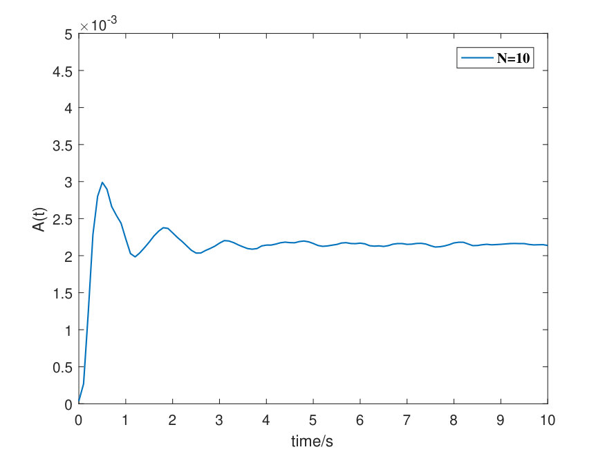 Figure 10
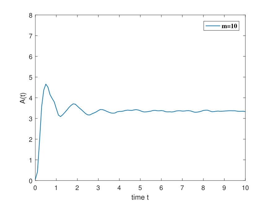 Figure 11
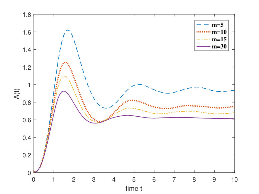 Figure 12
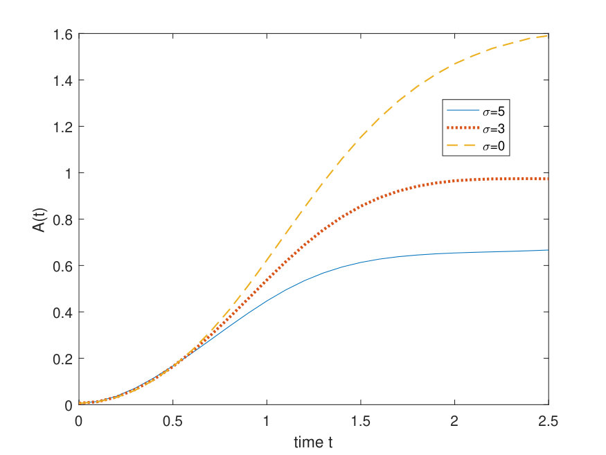 Figure 13
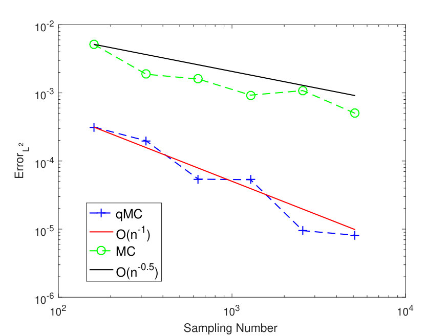 Figure 14
| Order | Order | |||
| 0.09862312 | 0.32096262 | |||
| 0.00129644 | 6.25 | 0.01449534 | 4.47 | |
| 0.00002892 | 5.49 | 0.00076150 | 4.25 | |
| 0.00000950 | 1.61 | 0.00014161 | 2.42 | |
Peer Reviews
No public reviews on file for this paper yet. If you reviewed it on a platform where reviews are public (OpenReview, ICLR, NeurIPS, ICML), you can paste yours below so the community can read it here.
Videos
No videos yet. Explain this paper in a talk, walkthrough, or lecture? Add one.
Taxonomy
TopicsAdvanced Mathematical Modeling in Engineering · Advanced Numerical Methods in Computational Mathematics · Numerical methods in inverse problems
A multiscale reduced basis method for Schrödinger equation with multiscale and random potentials
Jingrun Chen
Dingjiong Ma
Zhiwen Zhang
Mathematical Center for Interdisciplinary Research and School of Mathematical Sciences, Soochow University, Suzhou, China.
Department of Mathematics, The University of Hong Kong, Pokfulam Road, Hong Kong SAR, China.
Abstract
The semiclassical Schrödinger equation with multiscale and random potentials often appears when studying electron dynamics in heterogeneous quantum systems. As time evolves, the wavefunction develops high-frequency oscillations in both the physical space and the random space, which poses severe challenges for numerical methods. In this paper, we propose a multiscale reduced basis method, where we construct multiscale reduced basis functions using an optimization method and the proper orthogonal decomposition method in the physical space and employ the quasi-Monte Carlo method in the random space. Our method is verified to be efficient: the spatial gridsize is only proportional to the semiclassical parameter and the number of samples in the random space is inversely proportional to the same parameter. Several theoretical aspects of the proposed method, including how to determine the number of samples in the construction of multiscale reduced basis and convergence analysis, are studied with numerical justification. In addition, we investigate the Anderson localization phenomena for Schrödinger equation with correlated random potentials in both 1D and 2D.
Keyword: random Schrödinger equation; multiscale reduced basis function; optimization method; quasi-Monte Carlo method; Anderson localization.
AMS subject classifications. 35J10, 35Q41, 65M60, 65K10, 74Q10.
1 Introduction
The semiclassical Schrödinger equation describes electron dynamics in the semiclassical regime. Applications of such an equation can be found in Bose-Einstein condensation, graphene, semiconductors, topological insulators, etc. When propagating in a (quasi-)periodic microstructure, electrons experience a multiscale potential. As a consequence, the electron wavefunction develops high-frequency oscillations, which poses severe challenges from the numerical perspective. Brute-force methods are very costly and asymptotics-based methods have been proposed in the literature; see [jin2011mathematical] for review and references therein.
In [Anderson:58], Anderson proposed to study localized eigenstates in a tight-binding model with random potentials. This model was soon to be generalized to the random Schrödinger equation, i.e., the Schrödinger equation with a random potential. In this case, electrons are found to be localized provided that the strength of randomness is sufficiently large. The randomness can be realized in an experiment by enhancing the disorder of impurities in a material. Due to the importance of this model, Anderson was awarded the Nobel Prize in physics in 1977. In the presence of multiscale and random potentials, the electron wavefunction develops high-frequency oscillations in both the physical space and the random space, making numerical approximations even more difficult.
In this paper, we study the following Schrödinger equation with random potential in the semiclassical regime
[TABLE]
where is an effective Planck constant describing the microscopic and macroscopic scale ratio, is the spatial dimension, is the given random potential, is the electron wavefunction, and is the initial data. Here is the spatial domain and .
Equation (1) can be used to model electron transport in a disordered medium in a single-electron picture where the electron interaction is ignored. It is customary to write the semiclassical Schrödinger equation and the multiscale and random potential with a single parameter . But there is no reason that the parameter of the multiscale and random potential should be the same as the semiclassical parameter; see §5 for details on the parameterization of the multiscale and random potential .
The existence of Anderson localization is closely related to the electron wavefunction in (1). To be specific, assume has zero mean with respect to the measure induced by and denote the second-order moment of the position density. When the strength of disorder is small, an electron undergoes a diffusion process with , . In the presence of a strong disorder, however, converges to a time-independent quantity, i.e., , which implies the localization of the electron and the system undergoes a metal-insulator transition [mott1990metal, Erdos:10]. When , localization always occurs for (1) with random potential [Anderson:58]. When , the situation becomes complicated. Some analytical results show that localization occurs when the strength of disorder is large [frohlich1983absence, aizenman1993localization]. This motivates us to study Anderson localization in the presence of correlated random potentials [nosov2019correlation].
When the potential is deterministic, i.e., , many numerical methods have been proposed; see [bao2002time, faou2006poisson, tanushev2007mountain, jin2008gaussian, faou2009computing, delgadillo2016gauge, chen2019multiscale] for example. When the potential is random, few works have been done; see [wu2016bloch, jin2019gaussian]. As mentioned above, the major difficulty is that the wavefunction develops high-frequency oscillations in both the physical space and the random space, which requires tremendous computational resources.
Our work is motivated by the multiscale finite element method (FEM) for solving elliptic problems with multiscale coefficients [hou1999convergence, efendiev2009multiscale]. The multiscale FEM is capable of correctly capturing the large scale components of the multiscale solution on a coarse grid without accurately resolving all the small scale features in the solution. This is accomplished by incorporating the local microstructures of the differential operator into the multiscale FEM basis functions. Recently, several relevant works on constructing localized basis functions that approximate the elliptic operator with heterogeneous coefficients have been proposed. In [maalqvist2014localization], Malqvist and Peterseim construct localized multiscale basis functions using a modified variational multiscale method. The exponentially decaying property of these modified basis has been shown both theoretically and numerically. Meanwhile, Owhadi [Owhadi:2015, owhadi2017multigrid] reformulates the multiscale problem from the perspective of decision theory using the idea of gamblets as the modified basis. Hou et.al. [hou2017sparse] extend these works such that localized basis functions can also be constructed for higher-order strongly elliptic operators. Recently, Hou, Ma, and Zhang propose to build localized multiscale stochastic basis to solve elliptic problems with multiscale and random coefficients [hou2018model].
In this paper, we propose a multiscale reduced basis method to solve the Schrödinger equation with random potentials in the semiclassical regime. Our method consists of offline and online stages. In the offline stage, we apply an optimization approach to systematically construct localized multiscale reduced basis functions on each patch associated with each coarse gridpoint. These basis functions provide nearly optimal approximation to the random Schrödinger operator. In the online stage, we use these basis functions to approximate the physical space of the solution and the quasi-Monte Carlo (qMC) method to approximate the random space of the solution, respectively. We find the proposed method is efficient in the sense that the number of basis functions is only proportional to and the number of samples in qMC is inversely proportional to . Under some conditions, we conduct the convergence analysis of the proposed method with numerical verifications. Moreover, we study how to determine the number of samples in qMC such that the corresponding multiscale reduced basis functions provide accurate approximation of the solution space. Finally we investigate the existence of Anderson localization for correlated random potentials.
The rest of the paper is organized as follows. For completeness, in §2, we introduce multiscale basis functions for the deterministic Schrödinger equation in semiclassical regime and discuss some properties of the basis functions. In §3, we propose a multiscale reduced basis method to solve the random Schrödinger equation. Analysis results are presented in §4 and numerical experiments, including both 1D and 2D examples, are conducted to demonstrate the convergence and efficiency of the proposed method in §5. Conclusions and discussions are drawn in §LABEL:sec:Conclusion.
2 Multiscale basis functions for deterministic Schrödinger equations
In this section, we briefly review the construction of multiscale basis functions based on an optimization approach to solve the Schrödinger equation with a deterministic potential. Some properties of the multiscale basis functions are also given.
2.1 Construction of multiscale basis functions
In the deterministic case, we consider the following problem
[TABLE]
is the initial data over . Defining the Hamiltonian operator and introducing the following energy notation for Hamiltonian operator
[TABLE]
Note that (3) does not define a norm since usually can be negative, and thus the bilinear form associated to this notation is not coercive, which is quite different from the case of elliptic equations. However, this does not mean that available approaches [hou1997multiscale, babuska2011optimal, maalqvist2014localization, owhadi2017multigrid, hou2017sparse] cannot be used for the Schrödinger equation. In fact, we shall utilize the similar idea to construct localized multiscale basis functions on a coarse mesh by an optimization approach using the above energy notation for the Hamiltonian operator.
To construct such localized multiscale basis functions, we first partition the physical domain into a set of regular coarse elements with mesh size . For example, we divide into a set of non-overlapping triangles , such that no vertex of one triangle lies in the interior of the edge of another triangle. On each element , we define a set of nodal basis with being the number of nodes of the element. From now on, we neglect the subscript for notational convenience. The functions are called measurement functions, which are chosen as the characteristic functions on each coarse element in [hou2017sparse, owhadi2017multigrid] and piecewise linear basis functions in [maalqvist2014localization]. In [li2017computing, hou2018model], it is found that the usage of FEM nodal basis functions reduces the approximation error and thus the same setting is adopted in the current work.
Let denote the set of vertices of (removing the repeated vertices due to the periodic boundary condition) and be the number of vertices. For every vertex , let denote the corresponding nodal basis function, i.e., . Since all the nodal basis functions are continuous across the boundaries of the elements, we have
[TABLE]
Then, we can solve optimization problems to obtain the multiscale basis functions. Specifically, let be the minimizer of the following constrained optimization problem
[TABLE]
The superscript is dropped for notation simplicity and the periodic boundary condition is incorporated into the above optimization problem through the solution space .
In general, one cannot solve the above optimization problem analytically. Therefore, we use numerical methods to solve it. Specifically, we partition the physical domain into a set of non-overlapping fine triangles with size . Then, we use standard FEM to discretize , , . In the discrete level, the optimization problem (4)-(5) is reduced to a constrained quadratic optimization problem; see (19) in Section 3.3, which can be efficiently solved using Lagrange multiplier methods. Finally, with these multiscale FEM basis functions , we can solve the Schrödinger equation (2) using the Galerkin method.
Remark 2.1*.*
In analogy to the multistate FEM [hou1999convergence, efendiev2009multiscale], the multiscale basis functions are defined on coarse elements with mesh size . However, they are represented by fine-scale FEM basis with mesh size , which can be pre-computed and done in parallel.
Remark 2.2*.*
The notation in (3) does not define a norm. However, as long as the potential is bounded from below and the fine mesh size is small enough, the discrete problem of (4) - (5) is convex and thus admits a unique solution; see [hou2017sparse, li2017computing] for details.
2.2 Exponential decay of the multiscale finite element basis functions
It can be proved that the multiscale basis functions decay exponentially fast away from its associated vertex under certain conditions. This allows us to localize the basis functions to a relatively smaller domain and reduce the computational cost. We first define a series of nodal patches associated with as
[TABLE]
Assumption 2.1**.**
We assume the potential is bounded, i.e., and the mesh size of satisfies
[TABLE]
where means bounded from above by a constant.
Under this resolution assumption for the coarse mesh, many typical potentials in the Schrödinger equation (2) can be treated as a perturbation to the kinetic operator. Thus, they can be computed using our method. Then, we can show that the multiscale finite element basis functions have the exponentially decaying property.
Proposition 2.2** (Exponentially decaying property).**
Under the resolution condition of the coarse mesh, i.e., (8), there exist constants and independent of , such that
[TABLE]
for any .
Proof of (9) will be given in [ChenMaZhang:prep]. The main idea is to combine an iterative Caccioppoli-type argument [maalqvist2014localization, li2017computing] and some refined estimates with respect to .
The exponential decay of the basis functions enables us to localize the support sets of the basis functions , so that the corresponding stiffness matrix is sparse and the computational cost is reduced. In practice, we define a modified constrained optimization problem as follows
[TABLE]
where is the support set of the localized multiscale basis function and the choice of the integer depends on the decaying speed of . In (11) and (12), we have used the fact that has the exponentially decaying property so that we can localize the support set of to a smaller domain . In numerical experiments, we find that a small integer will give accurate results, where is the diameter of domain . Moreover, the optimization problem (10)-(12) can be solved in parallel. Therefore, the exponentially decaying property significantly reduces our computational cost in constructing basis functions and computing the solution of the Schrödinger equation (2).
With the localized multiscale finite element basis functions , we can approximate the wavefunction by using the Galerkin method.
3 Multiscale reduced basis functions for the random Schrödinger equation
3.1 Parametrization of the random potential
The random potential is used to model the disorder in a given material. Specifically, we assume is a second order random field, i.e., , with mean and covariance kernel . For example, we can choose the covariance kernel as
[TABLE]
where is a constant and ’s are the correlation lengths in each dimension. We also assume that the random potential is almost surely bounded, namely there exist and , such that
[TABLE]
Circulant embedding method [circulantEmbed1997] and Karhunen-Loève (KL) expansion method [Karhunen:47, Loeve:78] are commonly used to generate samples of , and the latter will be used in the current work. The KL expansion of reads as
[TABLE]
where ’s are mean-zero and uncorrelated random variables, i.e., , , and are the eigenpairs of the covariance kernel . Generally, ’s are sorted in a descending order and their decay rates depend on the regularity of the covariance kernel. It has been proven that an algebraic decay rate, i.e. , is achieved asymptotically if the covariance kernel is of finite Sobolev regularity, and an exponential decay rate is achieved, i.e., for some , if the covariance kernel is piecewisely analytic [schwab2006karhunen].
In practice, we truncate the KL expansion (15) into its first terms and obtain a parametrization of the random potential as
[TABLE]
which will be used in both analysis and numerics in the remaining part of the paper.
Remark 3.1*.*
In general, the decay rate of depends on the correlation lengths , of the random field . Small correlation length results in slow decay of the eigenvalues. When the correlation lengths approach zero, the random field becomes a spatially white noise, which is the case used in the original physics paper [Anderson:58].
3.2 Construction of the multiscale reduced basis functions
For the random Schrödinger equation (1), it is prohibitively expensive to construct multiscale basis functions for each realization of the random potential using (10) - (12). To address this issue, we use a model reduction method to build a small number of reduced basis functions that enable us to obtain multiscale basis functions in a cheaper way without loss of approximation accuracy.
For every , we first compute a set of samples of multiscale basis functions associated to the vertex . Specifically, let be samples of the random potential that are obtained using Monte Carlo (MC) method or qMC method, where is the number of samples. Denote the sample mean of the basis functions, and is the fluctuation of the th basis function.
We apply the proper orthogonal decomposition (POD) method [berkooz1993proper, sirovich1987turbulence] to and build a set of basis functions with that optimally approximates . Quantitatively, we have the following approximating property.
Proposition 3.1**.**
*Let be positive eigenvalues of the covariance kernel associated with the snapshot of the fluctuations and the corresponding eigenfunctions are , …, ,…. Then, the reduced basis functions have the following approximation property *
[TABLE]
where or and the number is determined according to the ratio .
In practice, we choose the first dominant reduced basis functions such that is close enough to to achieve a desired accuracy, say . More details of the POD method can be found in [berkooz1993proper, sirovich1987turbulence]. Notice that reduced basis functions and , approximately capture the mean profile and the fluctuation of multiscale basis functions associated with , respectively. Thus, it is expected that for each realization of the random potential the associated multiscale basis functions can be approximated by the reduced basis functions, i.e.,
[TABLE]
Remark 3.2*.*
To construct the multiscale reduced basis functions, we partition the coarse grids into fine-scale quadrilateral elements with meshsize , which requires additional computational cost in the offline stage. However, the precomputed reduced basis functions can be used repeatedly to solve (1) for each realization of the random potential and different initial data, which results in considerable savings.
3.3 Estimation of the number of learning samples
We shall study the continuous dependence of multiscale basis functions on the random potential, which provide a guidence on how to determine the number of samples in the construction of multiscale basis functions. For notational simplification, we carry out the analysis for multiscale basis functions without localization.
Let , denote the finite element basis functions defined on fine mesh with size and is the number of fine-scale finite element basis functions. When we numerically solve (4)-(5), we represent the multiscale basis function as and obtain the following quadratic programming problem with equality constraints
[TABLE]
where is the coefficients and is a symmetric positive definite matrix on the fine triangularization with the component
[TABLE]
In (19), is an -by- matrix with and an -by- vector with only the th entry being and others being [math].
The following result states the continuous dependence of multiscale basis functions on the random potential.
Theorem 3.2**.**
Assume the random potential is almost surely bounded, i.e. (14) is satisfied and mesh size of the fine-scale triangles is small such that: (1) is small; and (2) . Then for two realizations and of the random potential , the corresponding multiscale basis functions satisfy
[TABLE]
where the constant is independent of , and .
Proof.
Under the assumptions that is almost surely bounded and is small, we know that is a positive definite matrix. Moreover, we know that has full rank, i.e., . Therefore, the quadratic optimization problem (19) has a unique minimizer, satisfying the Karush-Kuhn-Tucker condition. Specifically, the unique minimizer of (19) can be explicitly written as
[TABLE]
For two realizations and , we define . Then
[TABLE]
and thus
[TABLE]
We choose to be small enough such that , and have
[TABLE]
and thus
[TABLE]
Therefore,
[TABLE]
By their definitions, we have
[TABLE]
and thus
[TABLE]
We complete the proof since and . ∎
Equipped with Theorem 3.2, we can estimate the number of samples in the construction of multiscale reduced basis functions. Suppose the random potential is of the form (16). For any , we choose an integer and a set of random samples such that
[TABLE]
where the expectation is taken over the random variables in of the form (16). We can give a way to choose the random samples since the distribution of the random variables , is known.
For every , let be the samples of multiscale basis functions associated with . Then, we have
[TABLE]
Given parameters and , we choose and so that the right-hand side of (26) is small. Then the space of multiscale basis functions can be well approximated by the samples of multiscale basis functions with controllable accuracy and the POD method is further applied to construct multiscale reduced basis functions.
3.4 Derivation of our method based on the multiscale reduced basis functions
In this section, we present our method for solving the random Schrödinger equation: in the physical space, we use the multiscale reduced basis functions obtained in §3.2; in the random space, we use the qMC method.
The implementation of the qMC method is fairly easy. For instance, given a set of qMC samples, expectation of the solution is approximated by
[TABLE]
where is the number of qMC samples. Details of the generation of qMC samples and its convergence analysis will be discussed in §4.
Now, we focus on how to approximate the wavefunction in the physical space for each qMC sample . For each node point , we have constructed a set of multiscale reduced basis functions and represent the wavefunction by
[TABLE]
where is the number of multiscale reduced basis functions associated with the node . In the Galerkin formulation, we have the following weak form
[TABLE]
where is a deterministic operator. To numerically solve (29), we introduce some notations. Let , , and be matrices with dimension . Their entries are given by
[TABLE]
Then, we can reduce the weak formulation (29) into the following ODE system
[TABLE]
where the column vector consisting of all expansion coefficients of the solution onto multiscale reduced basis functions. We can further rewrite (30) as
[TABLE]
where and . In the end, we can solve the above ODE system using existing ODE solvers.
Before ending this section, we shall explain why we choose the qMC method to approximate the random space of the electron wavefunction. Since the parameterization of a random potential may have high dimension, i.e., is large in (15), non-intrusive methods, such as sparse grid method [bungartz2004sparse] and stochastic collocation method [nobile2008sparse], become prohibitively expensive to solve PDEs with random coefficients. Polynomial chaos expansion (PCE) methods [ghanem2003stochastic, xiu2003modeling] are also frequently used in the literature to solve PDEs with random coefficients. This type of methods is useful if the solution is sufficiently smooth in the random space with small dimensionality. The performance of MC method does not depend on the dimension of the random space. However, its convergence rate is merely . The convergence rate of the qMC method is better both theoretically and numerically; see (45) in Theorem 4.5. Therefore, we choose the qMC method and its implementation is almost the same as the MC method.
4 Convergence analysis
We shall analyze the approximation error of the proposed method, where the emphasis is put on computing functionals of the wavefunction.
4.1 Regularity of the wavefunction with respect to the random variables
Since the potential in (1) is parametrized by random variables , in (16), i.e., . The wavefunction satisfies
[TABLE]
The Doob-Dynkin’s lemma implies the wavefunction in (32) can also be represented by a functional of these random variables, i.e., .
First of all, we analyze the error introduced by the parameterization of the random potential. We have the following estimate result.
Lemma 4.1**.**
The difference between wavefunctions to (32) and (1) satisfies
[TABLE]
Proof.
The difference satisfies
[TABLE]
By a direct calculation, we have
[TABLE]
where is the probability measure induced by the randomness in the potential (16) and thus
[TABLE]
Therefore, we obtain
[TABLE]
which completes the proof. ∎
To analyze the qMC method, it is crucial to bound the mixed first derivatives of with respect to . Denote for convenience. Let denote a multi-index of non-negative integers, with and . The value of determines the number of derivatives to be taken with respect to , and denotes the mixed derivative of with respect to all variables specified by the multi-index .
Lemma 4.2**.**
For any , any time , and for any multi-index with , the partial derivative of satisfies the following a-priori estimate
[TABLE]
Proof.
When , we take the derivative of (32) with respect to . Let and , we have
[TABLE]
Thereafter, we have the following estimate by a direction calculation
[TABLE]
and
[TABLE]
When , we have
[TABLE]
According to the definition of the random potential (15), we have if . Thus the above equation can be simplified as
[TABLE]
Similarly, we obtain
[TABLE]
and
[TABLE]
Now we are ready to prove the theorem by mathematical induction. From (35), we know that (34) holds for . Assume that (34) holds for with . Substituting this into (36) yields the desired estimate for the case. ∎
Remark 4.1*.*
The above derivation is similar to that in [jin2019gaussian], where an estimate in norm is obtained. Here, for each random realization , we have the esitmate (34) in norm, which will be used to prove the convergence in qMC.
4.2 Main result of the error analysis
In the framework of uncertainty quantification, we are interested in computing some statistical quantities of the electron wavefunction. As such, we shall present the error analysis of our method in computing functionals of .
Let be a continuous linear functional on , then there exists a constant such that
[TABLE]
for all . Consider the following integral
[TABLE]
with . We approximate the integral over the unit cube by randomly shifted lattice rules
[TABLE]
where is the (deterministic) generating vector and is the random shift which is uniformly distributed over . Notice that is the dimension of the random vector in the random potential and is the number of the sample point in implementing the qMC method. The interested reader is referred to [dick2013high] for more details of the randomly shifted lattice rules in the qMC method.
Lemma 4.3**.**
Let be the integrand in (37). Given with , weights , a randomly shifted lattice rule with points in dimensions can be constructed by a component-by-component algorithm such that, for all ,
[TABLE]
with
[TABLE]
Proof.
The proof of this result is essentially an application of the Koksma-Hlawka inequality, which is the same as the proofs of Theorem 15, Theorem 16, and Theorem 17 in [graham2015quasi], or Theorem 5.10 in [dick2013high] with the following modification of estimates:
[TABLE]
with the Riemann zeta function, and . ∎
To analyze the error of our method, we need to make some assumptions on the regularity of the eigenfunctions and the decay rate of the eigenvalues in the KL expansion (16) of the random potential.
Assumption 4.4**.**
- (a)
\let
0
There exist and such that for ; 2. (b)
\let
0
The Karhunen-Loéve eigenfunctions are continuous and there exist and such that for ; 3. (c)
\let
0
The sequence defined by satisfies for some , and for .
Recall that and are solutions to (1) and (32), respectively. Denote the solution obtained by our method using the multiscale reduced basis functions in the physical space and the qMC method in the random space. Under the assumptions for the random potential, we have the error estimate.
Theorem 4.5**.**
Consider the approximation of via qMC multiscale finite element methods, denoted by , where we assume . A randomly shifted lattice rule is applied to . Then, we can bound the root-mean-square error with respect to the uniformly distributed shift by
[TABLE]
for , and with for and for , with arbitrarily small. Here the constant is independent of , , and but depends on .
Proof.
The linearity of operator implies
[TABLE]
Under the assumption , we have, see for example [ChenMaZhang:prep],
[TABLE]
Under the assumptions (b) and (c) in Assumption 4.4, we have, based on Lemma 4.1,
[TABLE]
for all . Detailed derivation is essentially the same as the proof of Theorem 8 in [graham2015quasi].
Finally, when applying the qMC method to (42), we need to analyze the error in the qMC method. We adopt the standard framework, i.e., the Koksma-Hlawka inequality. Under Assumption 4.4, we have, based on Lemma 4.2 and Lemma 4.3,
[TABLE]
where for and for , with arbitrarily small. Detailed derivation is essentially the same as the proof of Theorem 20 in [graham2015quasi]. A combination of above estimates completes the proof. ∎
Remark 4.2*.*
The term in the error estimate (41) can be viewed as a modeling error. When the -term KL truncation potential in (16) provides an accurate approximation to the potential , the term becomes small or negligible.
Remark 4.3*.*
In §5, we will show the proposed method works well for a large class of random potentials, even when the eigenvalues in the KL expansion have a relatively slow decay rate. Therefore, Assumption 4.4 is a rather technical assumption for the convergence analysis of the proposed method.
Remark 4.4*.*
In the error analysis for the qMC method, we assume for notational convenience; see (37), where are i.i.d. uniform random variables. In the KL expansion (16) representation for , we choose , so that the conditions , are satisfied. The same convergence result can be obtained with little modification of the current proof.
5 Numerical examples
In this section, we conduct numerical experiments to test the accuracy and the efficiency of our method. Specifically, we will present convergence tests with respect to the physical meshsize, the number of multiscale reduced basis functions, and the number of qMC samples. In addition, we will investigate the existence of Anderson localization in both 1D and 2D. For convenience, we first introduce norm and norm as
[TABLE]
In what follows, we compare the relative error between expectations of the numerical solution and the reference solution in both norm and norm
[TABLE]
Here , , is the random space, and is the probability measure induced by the randomness in (16). The reference solution refers to the numerical wavefunction using a very fine mesh and a large amount of qMC samples. In numerical experiments, we use the MATLAB’s Statistics Toolbox to generate the Sobol sequence to implement the qMC method. When we use the POD method to construct multiscale reduced basis functions, we observed similar decay behaviors of the associated eigenvalues at each coarse grid point. Therefore, we choose the same reduced basis number for all the coarse grid points.
5.1 Convergence in the physical space
Consider the 1D Schrödinger equation over
[TABLE]
where the periodic condition is imposed, the initial data , and the random potential is defined as
[TABLE]
In the random potential (47), is used to control the strength of the random potential, and ’s are mean-zero and independent random variables uniformly distributed in . Moreover, we choose , and , i.e., the characteristic length scale of randomness is different from the semiclassical parameter.
Convergence with respect to the coarse mesh size . In our numerical test, we set the final computational time . For the reference solution, we choose the fine mesh to be and the qMC sample number to be . For our method, we choose the POD modes , the sampling number in the offline training stage to be and the number of qMC samples in the online stage to be .
In Table LABEL:table_physical, we compute the relative errors of the expectation of the wavefunction in both norm and norm for a series of coarse meshes with meshsize ranging from to . Nice convergence in the physical space is observed.