Bimetric interactions based on metric congruences
Mikica Kocic

TL;DR
This paper introduces a new approach to defining spin-2 interactions in massive gravity and bigravity using a congruence matrix, providing insights into the mathematical structure and equivalences of different formulations.
Contribution
It presents a novel construction of bimetric interactions via a congruence matrix, establishing the uniqueness of the primary square root solution and linking metric and vielbein formulations.
Findings
Primary square root matrix is the unique power series solution.
Shift vector redefinition arises naturally from equations of motion.
Bimetric congruence formulation is algebraically equivalent to the vielbein approach.
Abstract
In massive gravity and bigravity, spin-2 interactions are defined in terms of a square root matrix that involves two metrics. In this work, the interactions are constructed using a congruence matrix between the metrics. It is established that the primary square root matrix function is the only power series solution to the equations of motion for the congruence. Moreover, the shift vector redefinition that is used in the bimetric ghost-free proofs follows from the form of the equations of motion. The analysis also gives an insight into the vielbein formulation of spin-2 interactions since the bimetric formulation in terms of a congruence is algebraically equivalent to the unconstrained vielbein formulation.
Click any figure to enlarge with its caption.
 Figure 1
 Figure 2
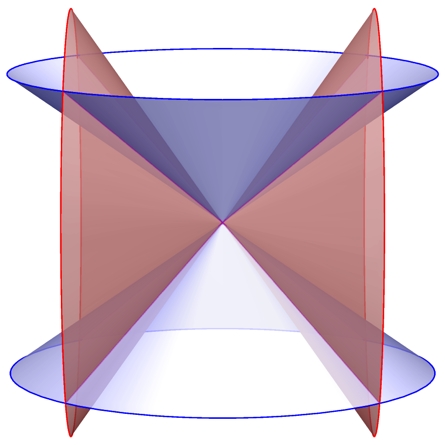 Figure 1
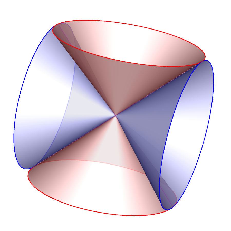 Figure 1
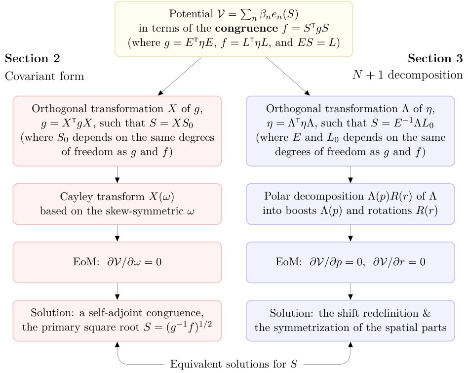 Figure 2
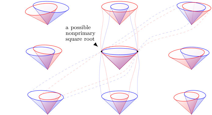 Figure 3
| , | , | , | , | , | , | ||||
| , | , | , | , | , | , | ||||
| , | , | , | , | , | , | ||||
| , | , | , | , | , | , | ||||
| , | , | , | , | , | |||||
| , | , | , | , | , | , | ||||
| , | , | , | . |
Peer Reviews
No public reviews on file for this paper yet. If you reviewed it on a platform where reviews are public (OpenReview, ICLR, NeurIPS, ICML), you can paste yours below so the community can read it here.
Videos
No videos yet. Explain this paper in a talk, walkthrough, or lecture? Add one.
Taxonomy
TopicsCosmology and Gravitation Theories · Black Holes and Theoretical Physics · Noncommutative and Quantum Gravity Theories
††institutetext: Department of Physics & The Oskar Klein Centre,
Stockholm University, AlbaNova University Centre, SE-106 91 Stockholm
Bimetric interactions based on metric congruences
Mikica Kocic
Abstract
In massive gravity and bigravity, spin-2 interactions are defined in terms of a square root matrix that involves two metrics. In this work, the interactions are constructed using a congruence matrix between the metrics. It is established that the primary square root matrix function is the only power series solution to the equations of motion for the congruence. Moreover, the shift vector redefinition that is used in the bimetric ghost-free proofs follows from the form of the equations of motion. The analysis also gives an insight into the vielbein formulation of spin-2 interactions since the bimetric formulation in terms of a congruence is algebraically equivalent to the unconstrained vielbein formulation.
Keywords:
Modified gravity, Massive gravity, Bigravity, Ghost-free bimetric theory
1 Introduction
General relativity is the classical theory of nonlinear self-interactions for a massless spin-2 field governed by the Einstein–Hilbert action. The context of this paper are its extensions: de Rham–Gabadadze–Tolley (dRGT) massive gravity deRham:2010kj ; Hassan:2011hr ; Hassan:2011tf and the Hassan–Rosen (HR) bimetric theory or bigravity Hassan:2011zd ; Hassan:2011ea ; Hassan:2018mbl . Massive gravity is a nonlinear theory of a single massive spin-2 field, while bigravity is a nonlinear theory of two interacting spin-2 fields having both massless and massive modes. These theories have been studied extensively over the past years; for reviews, see deRham:2014zqa ; Hinterbichler:2011tt ; Schmidt-May:2015vnx .
Massive gravity and bigravity are classically consistent theories, free of instabilities such as the Boulware–Deser ghost Boulware:1973my . This is not a coincidence, but due to the particular structure of the bimetric scalar potential proposed in deRham:2010kj with a compact general form Hassan:2011tf ,
[TABLE]
The potential involves two metric fields {\color[rgb]{0,0,0}\definecolor[named]{pgfstrokecolor}{rgb}{0,0,0}\pgfsys@color@gray@stroke{0}\pgfsys@color@gray@fill{0}g} and {\color[rgb]{0,0,0}\definecolor[named]{pgfstrokecolor}{rgb}{0,0,0}\pgfsys@color@gray@stroke{0}\pgfsys@color@gray@fill{0}f}; it is specifically constructed in terms of the square root matrix ({\color[rgb]{0,0,0}\definecolor[named]{pgfstrokecolor}{rgb}{0,0,0}\pgfsys@color@gray@stroke{0}\pgfsys@color@gray@fill{0}g}^{-1}{\color[rgb]{0,0,0}\definecolor[named]{pgfstrokecolor}{rgb}{0,0,0}\pgfsys@color@gray@stroke{0}\pgfsys@color@gray@fill{0}f})^{1/2} using the elementary symmetric polynomials macdonald:1998a , where the interaction is parametrized by constants . In massive gravity, the metric {\color[rgb]{0,0,0}\definecolor[named]{pgfstrokecolor}{rgb}{0,0,0}\pgfsys@color@gray@stroke{0}\pgfsys@color@gray@fill{0}g} carries dynamics while {\color[rgb]{0,0,0}\definecolor[named]{pgfstrokecolor}{rgb}{0,0,0}\pgfsys@color@gray@stroke{0}\pgfsys@color@gray@fill{0}f} is a reference nondynamical field. In bigravity, both {\color[rgb]{0,0,0}\definecolor[named]{pgfstrokecolor}{rgb}{0,0,0}\pgfsys@color@gray@stroke{0}\pgfsys@color@gray@fill{0}g} and {\color[rgb]{0,0,0}\definecolor[named]{pgfstrokecolor}{rgb}{0,0,0}\pgfsys@color@gray@stroke{0}\pgfsys@color@gray@fill{0}f} are dynamical, each having its own Einstein–Hilbert term.
The vielbein formulation of spin-2 interactions was constructed in Hinterbichler:2012cn . The vielbein based potential has the following expression (given in Hinterbichler:2012cn , cf. Zumino:1970tu ),
[TABLE]
Here, denotes the Levi–Civita symbol, and the vielbeins are represented by one-forms {\color[rgb]{0,0,0}\definecolor[named]{pgfstrokecolor}{rgb}{0,0,0}\pgfsys@color@gray@stroke{0}\pgfsys@color@gray@fill{0}E}^{A}={\color[rgb]{0,0,0}\definecolor[named]{pgfstrokecolor}{rgb}{0,0,0}\pgfsys@color@gray@stroke{0}\pgfsys@color@gray@fill{0}E}{}^{A}{}_{\mu}\mathrm{d}x^{\mu} and {\color[rgb]{0,0,0}\definecolor[named]{pgfstrokecolor}{rgb}{0,0,0}\pgfsys@color@gray@stroke{0}\pgfsys@color@gray@fill{0}L}^{A}={\color[rgb]{0,0,0}\definecolor[named]{pgfstrokecolor}{rgb}{0,0,0}\pgfsys@color@gray@stroke{0}\pgfsys@color@gray@fill{0}L}{}^{A}{}_{\mu}\mathrm{d}x^{\mu}. The associated metrics are,
[TABLE]
where is the metric of the local Lorentz frame. In the constrained version, h=\eta_{AB}{\color[rgb]{0,0,0}\definecolor[named]{pgfstrokecolor}{rgb}{0,0,0}\pgfsys@color@gray@stroke{0}\pgfsys@color@gray@fill{0}L}^{A}{\color[rgb]{0,0,0}\definecolor[named]{pgfstrokecolor}{rgb}{0,0,0}\pgfsys@color@gray@stroke{0}\pgfsys@color@gray@fill{0}E}^{B} is symmetric, which is equivalent to having a real square root ({\color[rgb]{0,0,0}\definecolor[named]{pgfstrokecolor}{rgb}{0,0,0}\pgfsys@color@gray@stroke{0}\pgfsys@color@gray@fill{0}g}^{-1}{\color[rgb]{0,0,0}\definecolor[named]{pgfstrokecolor}{rgb}{0,0,0}\pgfsys@color@gray@stroke{0}\pgfsys@color@gray@fill{0}f})^{1/2}={\color[rgb]{0,0,0}\definecolor[named]{pgfstrokecolor}{rgb}{0,0,0}\pgfsys@color@gray@stroke{0}\pgfsys@color@gray@fill{0}E}^{-1}{\color[rgb]{0,0,0}\definecolor[named]{pgfstrokecolor}{rgb}{0,0,0}\pgfsys@color@gray@stroke{0}\pgfsys@color@gray@fill{0}L} in matrix notation Deffayet:2012zc . Consequently, the constrained vielbein formulation is equivalent to the metric formulation since (1) and (2) become equal. The metric formulation of the multivielbein theory was treated in Hassan:2012wt .
Purpose of this work.
We address several issues related to bimetric interactions. First, the question if there exists a more general bimetric formulation of the potential (1) yet equivalent to the vielbein formulation that is based the symmetric polynomials; then, if it exists, what governs the selection of the square root in the constrained case? Namely, the square root matrix ({\color[rgb]{0,0,0}\definecolor[named]{pgfstrokecolor}{rgb}{0,0,0}\pgfsys@color@gray@stroke{0}\pgfsys@color@gray@fill{0}g}^{-1}{\color[rgb]{0,0,0}\definecolor[named]{pgfstrokecolor}{rgb}{0,0,0}\pgfsys@color@gray@stroke{0}\pgfsys@color@gray@fill{0}f})^{1/2} must represent a well-defined tensor field. Notwithstanding, it may have multiple branches, and besides not being real, it can be solved ad hoc from the matrix equation {\color[rgb]{0,0,0}\definecolor[named]{pgfstrokecolor}{rgb}{0,0,0}\pgfsys@color@gray@stroke{0}\pgfsys@color@gray@fill{0}g}^{-1}{\color[rgb]{0,0,0}\definecolor[named]{pgfstrokecolor}{rgb}{0,0,0}\pgfsys@color@gray@stroke{0}\pgfsys@color@gray@fill{0}f}=S^{2} which may have an infinite number of solutions (an example of such {\color[rgb]{0,0,0}\definecolor[named]{pgfstrokecolor}{rgb}{0,0,0}\pgfsys@color@gray@stroke{0}\pgfsys@color@gray@fill{0}g}^{-1}{\color[rgb]{0,0,0}\definecolor[named]{pgfstrokecolor}{rgb}{0,0,0}\pgfsys@color@gray@stroke{0}\pgfsys@color@gray@fill{0}f} is shown in figure 1b). In the vielbein formulation, the square root selection is concealed inside the symmetrization condition giving no definite choice for Deffayet:2012zc .
Another issue concerns the initial value problem for the unconstrained vielbein formulation. The ghost-free proof in Hinterbichler:2012cn assumes the simultaneous N+1 decomposition with arbitrarily boosted vielbeins. This is in general not possible since one cannot ensure that an arbitrary vielbein {\color[rgb]{0,0,0}\definecolor[named]{pgfstrokecolor}{rgb}{0,0,0}\pgfsys@color@gray@stroke{0}\pgfsys@color@gray@fill{0}L} can simultaneously be triangularized with {\color[rgb]{0,0,0}\definecolor[named]{pgfstrokecolor}{rgb}{0,0,0}\pgfsys@color@gray@stroke{0}\pgfsys@color@gray@fill{0}E} already being in the triangular form. A typical example is shown in figure 1a, where the null cones of the two metrics doubly intersect; in this case the simultaneous N+1 decomposition of {\color[rgb]{0,0,0}\definecolor[named]{pgfstrokecolor}{rgb}{0,0,0}\pgfsys@color@gray@stroke{0}\pgfsys@color@gray@fill{0}g} & {\color[rgb]{0,0,0}\definecolor[named]{pgfstrokecolor}{rgb}{0,0,0}\pgfsys@color@gray@stroke{0}\pgfsys@color@gray@fill{0}f}, and the simultaneous triangularization of {\color[rgb]{0,0,0}\definecolor[named]{pgfstrokecolor}{rgb}{0,0,0}\pgfsys@color@gray@stroke{0}\pgfsys@color@gray@fill{0}E} & {\color[rgb]{0,0,0}\definecolor[named]{pgfstrokecolor}{rgb}{0,0,0}\pgfsys@color@gray@stroke{0}\pgfsys@color@gray@fill{0}L}, are not possible.
Summary of results.
An overview of the paper with the key results is shown in figure 2.
In section 2, we construct bimetric interactions in terms of a general congruence {\color[rgb]{0,0,0}\definecolor[named]{pgfstrokecolor}{rgb}{0,0,0}\pgfsys@color@gray@stroke{0}\pgfsys@color@gray@fill{0}f}=S^{\mathsf{{\scriptscriptstyle T}}}{\color[rgb]{0,0,0}\definecolor[named]{pgfstrokecolor}{rgb}{0,0,0}\pgfsys@color@gray@stroke{0}\pgfsys@color@gray@fill{0}g}S between the metric fields {\color[rgb]{0,0,0}\definecolor[named]{pgfstrokecolor}{rgb}{0,0,0}\pgfsys@color@gray@stroke{0}\pgfsys@color@gray@fill{0}g} and {\color[rgb]{0,0,0}\definecolor[named]{pgfstrokecolor}{rgb}{0,0,0}\pgfsys@color@gray@stroke{0}\pgfsys@color@gray@fill{0}f}. This congruence based metric formulation is algebraically equivalent to the unconstrained vielbein formulation Hinterbichler:2012cn . We solve the equation of motion for the congruence, which necessarily gives the primary square root S=({\color[rgb]{0,0,0}\definecolor[named]{pgfstrokecolor}{rgb}{0,0,0}\pgfsys@color@gray@stroke{0}\pgfsys@color@gray@fill{0}g}^{-1}{\color[rgb]{0,0,0}\definecolor[named]{pgfstrokecolor}{rgb}{0,0,0}\pgfsys@color@gray@stroke{0}\pgfsys@color@gray@fill{0}f})^{1/2} as the congruence field. In section 3, the equations are solved using the N+1 decomposition. The obtained solution is the symmetrization of the spatial metrics together with the shift vector redefinition that was used in the bimetric ghost-free proofs Hassan:2011tf ; Hassan:2011zd . The rest of the introduction is devoted to a mathematical background on metric congruences.
Notation.
The metric signature is mostly positive . The spacetime dimension is . In the space-plus-time decomposition, , hats over spacetime objects denote their spatial restrictions. The equations are mostly written in matrix notation. Hence, the expressions are preferably stated using (1,1)-tensors with the default down-up contractions. Matrices do not naturally represent metrics and require transposes on the left side of the metric symbol in matrix notation. Examples of how to restore the indices are given in appendix A. Spacetime (world) indices are denoted by and their spatial restrictions by , while Lorentz (local frame) indices are denoted by and their spatial restrictions by .
1.1 Metric congruences
Here we review some basic properties of symmetric bilinear forms (metrics) and their isometries (congruent transformations or congruences); for more details see Scharlau:1985 ; Lang:2002 ; Meinrenken:2013 . Two examples of congruences are orthogonal transformations and moving frames (vielbeins).
Let {\color[rgb]{0,0,0}\definecolor[named]{pgfstrokecolor}{rgb}{0,0,0}\pgfsys@color@gray@stroke{0}\pgfsys@color@gray@fill{0}g} be a nondegenerate symmetric bilinear form on a finite-dimensional real vector space . The pair (V,{\color[rgb]{0,0,0}\definecolor[named]{pgfstrokecolor}{rgb}{0,0,0}\pgfsys@color@gray@stroke{0}\pgfsys@color@gray@fill{0}g}) is called a real symmetric bilinear space. Two symmetric bilinear spaces (V,{\color[rgb]{0,0,0}\definecolor[named]{pgfstrokecolor}{rgb}{0,0,0}\pgfsys@color@gray@stroke{0}\pgfsys@color@gray@fill{0}g}) and (\mkern 1.0mu\widetilde{\mkern-1.0muV},{\color[rgb]{0,0,0}\definecolor[named]{pgfstrokecolor}{rgb}{0,0,0}\pgfsys@color@gray@stroke{0}\pgfsys@color@gray@fill{0}f}) are isometric iff there exists an invertible linear transformation such that,
[TABLE]
That is, {\color[rgb]{0,0,0}\definecolor[named]{pgfstrokecolor}{rgb}{0,0,0}\pgfsys@color@gray@stroke{0}\pgfsys@color@gray@fill{0}f} is a precomposition of {\color[rgb]{0,0,0}\definecolor[named]{pgfstrokecolor}{rgb}{0,0,0}\pgfsys@color@gray@stroke{0}\pgfsys@color@gray@fill{0}g} with the map (or the pullback of {\color[rgb]{0,0,0}\definecolor[named]{pgfstrokecolor}{rgb}{0,0,0}\pgfsys@color@gray@stroke{0}\pgfsys@color@gray@fill{0}g} by ). This corresponds to the matrix congruence {\color[rgb]{0,0,0}\definecolor[named]{pgfstrokecolor}{rgb}{0,0,0}\pgfsys@color@gray@stroke{0}\pgfsys@color@gray@fill{0}f}=S^{\mathsf{{\scriptscriptstyle T}}}{\color[rgb]{0,0,0}\definecolor[named]{pgfstrokecolor}{rgb}{0,0,0}\pgfsys@color@gray@stroke{0}\pgfsys@color@gray@fill{0}g}S in some basis. In linear algebra, the linear transformation is usually referred to as an isometry. To avoid possible confusion with the Killing symmetries of the metric fields, we adopt another frequently used name “congruence” or “congruent transformation.” By Sylvester’s law of inertia, the congruent transformations preserve the signature of the symmetric bilinear forms. They form a group of automorphisms on the same vector space .
The point-wise notion of a congruence can be lifted from linear algebra to differential geometry (i.e., from a tensor to a tensor field). A possible obstruction is that the congruence field might not be defined as a global section of the fiber bundle. A typical example is a vielbein, which globally exists iff the manifold is parallelizable Hawking:1973large . Nevertheless, one can always assume the local existence of sections, which we employ here.
Adjoint maps.
Two linear transformations and are adjoint with respect to {\color[rgb]{0,0,0}\definecolor[named]{pgfstrokecolor}{rgb}{0,0,0}\pgfsys@color@gray@stroke{0}\pgfsys@color@gray@fill{0}g}, iff
[TABLE]
In matrix notation we have A^{\prime}={\color[rgb]{0,0,0}\definecolor[named]{pgfstrokecolor}{rgb}{0,0,0}\pgfsys@color@gray@stroke{0}\pgfsys@color@gray@fill{0}g}^{-1}A^{\mathsf{{\scriptscriptstyle T}}}{\color[rgb]{0,0,0}\definecolor[named]{pgfstrokecolor}{rgb}{0,0,0}\pgfsys@color@gray@stroke{0}\pgfsys@color@gray@fill{0}g}. This relation can be used to define the adjoint of (having a regular {\color[rgb]{0,0,0}\definecolor[named]{pgfstrokecolor}{rgb}{0,0,0}\pgfsys@color@gray@stroke{0}\pgfsys@color@gray@fill{0}g}). A self-adjoint transformation is such that . An example of self-adjoint transformations with respect to {\color[rgb]{0,0,0}\definecolor[named]{pgfstrokecolor}{rgb}{0,0,0}\pgfsys@color@gray@stroke{0}\pgfsys@color@gray@fill{0}g} are the matrix functions of {\color[rgb]{0,0,0}\definecolor[named]{pgfstrokecolor}{rgb}{0,0,0}\pgfsys@color@gray@stroke{0}\pgfsys@color@gray@fill{0}g}^{-1}{\color[rgb]{0,0,0}\definecolor[named]{pgfstrokecolor}{rgb}{0,0,0}\pgfsys@color@gray@stroke{0}\pgfsys@color@gray@fill{0}f}.
Orthogonal group.
An orthogonal transformation is a congruence whose adjoint is equal its inverse, . Beware that “adjointness” is always stated with respect to some symmetric bilinear form (here {\color[rgb]{0,0,0}\definecolor[named]{pgfstrokecolor}{rgb}{0,0,0}\pgfsys@color@gray@stroke{0}\pgfsys@color@gray@fill{0}g}). The orthogonal group \operatorname{O}(V,{\color[rgb]{0,0,0}\definecolor[named]{pgfstrokecolor}{rgb}{0,0,0}\pgfsys@color@gray@stroke{0}\pgfsys@color@gray@fill{0}g}) comprise all the automorphisms which preserve {\color[rgb]{0,0,0}\definecolor[named]{pgfstrokecolor}{rgb}{0,0,0}\pgfsys@color@gray@stroke{0}\pgfsys@color@gray@fill{0}g}, that is, {\color[rgb]{0,0,0}\definecolor[named]{pgfstrokecolor}{rgb}{0,0,0}\pgfsys@color@gray@stroke{0}\pgfsys@color@gray@fill{0}g}=X^{\mathsf{{\scriptscriptstyle T}}}{\color[rgb]{0,0,0}\definecolor[named]{pgfstrokecolor}{rgb}{0,0,0}\pgfsys@color@gray@stroke{0}\pgfsys@color@gray@fill{0}g}X. Note that a congruence between (\mkern 1.0mu\widetilde{\mkern-1.0muV},{\color[rgb]{0,0,0}\definecolor[named]{pgfstrokecolor}{rgb}{0,0,0}\pgfsys@color@gray@stroke{0}\pgfsys@color@gray@fill{0}f}) and (V,{\color[rgb]{0,0,0}\definecolor[named]{pgfstrokecolor}{rgb}{0,0,0}\pgfsys@color@gray@stroke{0}\pgfsys@color@gray@fill{0}g}) always contains excessive degrees of freedom because it can only be determined up to a residual orthogonal transformation of either {\color[rgb]{0,0,0}\definecolor[named]{pgfstrokecolor}{rgb}{0,0,0}\pgfsys@color@gray@stroke{0}\pgfsys@color@gray@fill{0}g} or {\color[rgb]{0,0,0}\definecolor[named]{pgfstrokecolor}{rgb}{0,0,0}\pgfsys@color@gray@stroke{0}\pgfsys@color@gray@fill{0}f}.
1.2 Parametrization of orthogonal transformations
A special orthogonal transformation can be parametrized by a skew-symmetric bilinear form {\color[rgb]{0,0,0}\definecolor[named]{pgfstrokecolor}{rgb}{0,0,0}\pgfsys@color@gray@stroke{0}\pgfsys@color@gray@fill{0}\omega}=-{\color[rgb]{0,0,0}\definecolor[named]{pgfstrokecolor}{rgb}{0,0,0}\pgfsys@color@gray@stroke{0}\pgfsys@color@gray@fill{0}\omega}^{\mathsf{{\scriptscriptstyle T}}} using the Cayley transform Golub:1996 ,
[TABLE]
It is straightforward to verify that {\color[rgb]{0,0,0}\definecolor[named]{pgfstrokecolor}{rgb}{0,0,0}\pgfsys@color@gray@stroke{0}\pgfsys@color@gray@fill{0}g}=X^{\mathsf{{\scriptscriptstyle T}}}{\color[rgb]{0,0,0}\definecolor[named]{pgfstrokecolor}{rgb}{0,0,0}\pgfsys@color@gray@stroke{0}\pgfsys@color@gray@fill{0}g}X={\color[rgb]{0,0,0}\definecolor[named]{pgfstrokecolor}{rgb}{0,0,0}\pgfsys@color@gray@stroke{0}\pgfsys@color@gray@fill{0}g}^{\mathsf{{\scriptscriptstyle T}}} since,
[TABLE]
The parametrization (6) is special since . In -dimensions, contains degrees of freedom in the components of {\color[rgb]{0,0,0}\definecolor[named]{pgfstrokecolor}{rgb}{0,0,0}\pgfsys@color@gray@stroke{0}\pgfsys@color@gray@fill{0}\omega}. Any can be factored as a noncommutative product of orthogonal transformations where each contains partial degrees of freedom in the corresponding skew-symmetric {\color[rgb]{0,0,0}\definecolor[named]{pgfstrokecolor}{rgb}{0,0,0}\pgfsys@color@gray@stroke{0}\pgfsys@color@gray@fill{0}\omega}_{i}.
The N+1 parametrization of boosts and rotations.
Here we present a recursive definition of the orthogonal transformation, which is useful to triangularize vielbeins in their entire form. The same procedure is implicitly employed in the Cholesky decomposition to factor positive definite matrices into the product of a lower triangular matrix and its transpose Golub:1996 ; see also the Cholesky–Banachiewicz and Cholesky–Crout algorithms Obsieger:2015nm2 .
Let be a -dimensional metric of either Lorentzian or Euclidean signature, where {\color[rgb]{0,0,0}\definecolor[named]{pgfstrokecolor}{rgb}{0,0,0}\pgfsys@color@gray@stroke{0}\pgfsys@color@gray@fill{0}\hat{\delta}} is its -dimensional restriction,
[TABLE]
The orthogonal transformation can be parametrized Meinrenken:2013 ,
[TABLE]
where is a -dimensional vector, {\color[rgb]{0,0,0}\definecolor[named]{pgfstrokecolor}{rgb}{0,0,0}\pgfsys@color@gray@stroke{0}\pgfsys@color@gray@fill{0}\hat{\delta}}={\color[rgb]{0,0,0}\definecolor[named]{pgfstrokecolor}{rgb}{0,0,0}\pgfsys@color@gray@stroke{0}\pgfsys@color@gray@fill{0}\hat{R}}^{\mathsf{{\scriptscriptstyle T}}}{\color[rgb]{0,0,0}\definecolor[named]{pgfstrokecolor}{rgb}{0,0,0}\pgfsys@color@gray@stroke{0}\pgfsys@color@gray@fill{0}\hat{\delta}}{\color[rgb]{0,0,0}\definecolor[named]{pgfstrokecolor}{rgb}{0,0,0}\pgfsys@color@gray@stroke{0}\pgfsys@color@gray@fill{0}\hat{R}} is an orthogonal transformation of the Euclidean restriction, {\color[rgb]{0,0,0}\definecolor[named]{pgfstrokecolor}{rgb}{0,0,0}\pgfsys@color@gray@stroke{0}\pgfsys@color@gray@fill{0}\hat{I}} is the identity map, and denotes an optional reflection (ignored in the following). The parameter space is confined to , which is satisfied for any in the Lorentzian case .
The factorization (9) is recursive. For and , we have where comprises three-parameter boosts of the 44 Minkowski metric, contains two-parameter rotations of the 33 Euclidean metric, and is a one-parameter rotation of the 22 Euclidean metric. This effectively gives a polar decomposition of the orthogonal transformation where the Lorentz boosts are parametrized by an arbitrary spatial Lorentz vector {\color[rgb]{0,0,0}\definecolor[named]{pgfstrokecolor}{rgb}{0,0,0}\pgfsys@color@gray@stroke{0}\pgfsys@color@gray@fill{0}p} (see Proposition 1.13 in Meinrenken:2013 ),
[TABLE]
The nonvanishing components of {\color[rgb]{0,0,0}\definecolor[named]{pgfstrokecolor}{rgb}{0,0,0}\pgfsys@color@gray@stroke{0}\pgfsys@color@gray@fill{0}\omega} in the corresponding Cayley parametrization (6) are {\color[rgb]{0,0,0}\definecolor[named]{pgfstrokecolor}{rgb}{0,0,0}\pgfsys@color@gray@stroke{0}\pgfsys@color@gray@fill{0}\omega}_{0a}={\color[rgb]{0,0,0}\definecolor[named]{pgfstrokecolor}{rgb}{0,0,0}\pgfsys@color@gray@stroke{0}\pgfsys@color@gray@fill{0}p}^{b}\delta_{ba}/({\color[rgb]{0,0,0}\definecolor[named]{pgfstrokecolor}{rgb}{0,0,0}\pgfsys@color@gray@stroke{0}\pgfsys@color@gray@fill{0}\lambda}+1). Also note that,
[TABLE]
The boosts can be reparametrized through {\color[rgb]{0,0,0}\definecolor[named]{pgfstrokecolor}{rgb}{0,0,0}\pgfsys@color@gray@stroke{0}\pgfsys@color@gray@fill{0}v}\coloneqq{\color[rgb]{0,0,0}\definecolor[named]{pgfstrokecolor}{rgb}{0,0,0}\pgfsys@color@gray@stroke{0}\pgfsys@color@gray@fill{0}p}/{\color[rgb]{0,0,0}\definecolor[named]{pgfstrokecolor}{rgb}{0,0,0}\pgfsys@color@gray@stroke{0}\pgfsys@color@gray@fill{0}\lambda} where,
[TABLE]
Similar expressions hold for rotations. For instance, reads,
[TABLE]
2 Congruence based bimetric scalar potential
We consider the scalar potential based on the elementary symmetric polynomials ,
[TABLE]
where is an arbitrary congruence between the metric fields {\color[rgb]{0,0,0}\definecolor[named]{pgfstrokecolor}{rgb}{0,0,0}\pgfsys@color@gray@stroke{0}\pgfsys@color@gray@fill{0}g} and {\color[rgb]{0,0,0}\definecolor[named]{pgfstrokecolor}{rgb}{0,0,0}\pgfsys@color@gray@stroke{0}\pgfsys@color@gray@fill{0}f},111 Note that (15) is not the most general congruence between {\color[rgb]{0,0,0}\definecolor[named]{pgfstrokecolor}{rgb}{0,0,0}\pgfsys@color@gray@stroke{0}\pgfsys@color@gray@fill{0}g} and {\color[rgb]{0,0,0}\definecolor[named]{pgfstrokecolor}{rgb}{0,0,0}\pgfsys@color@gray@stroke{0}\pgfsys@color@gray@fill{0}f} since the metrics can be on different manifolds. Then, to write (15), we need a diffeomorphism between the manifolds (with the pullback of one of the metrics), which in turn introduces a diagonal group of common diffeomorphisms. This generalization, however, does not affect the presented analysis (see appendix C for more details).
[TABLE]
The congruence is determined up to a local orthogonal transformation of {\color[rgb]{0,0,0}\definecolor[named]{pgfstrokecolor}{rgb}{0,0,0}\pgfsys@color@gray@stroke{0}\pgfsys@color@gray@fill{0}g},
[TABLE]
such that , where possibly depends on the degrees of freedom in {\color[rgb]{0,0,0}\definecolor[named]{pgfstrokecolor}{rgb}{0,0,0}\pgfsys@color@gray@stroke{0}\pgfsys@color@gray@fill{0}g} and {\color[rgb]{0,0,0}\definecolor[named]{pgfstrokecolor}{rgb}{0,0,0}\pgfsys@color@gray@stroke{0}\pgfsys@color@gray@fill{0}f}, but not on . The additional components of the congruence are removed by on-shell conditions for . All the fields are assumed to be regular since any singularity punctures the manifold.
The orthogonal transformation can be parametrized by a skew-symmetric tensor field {\color[rgb]{0,0,0}\definecolor[named]{pgfstrokecolor}{rgb}{0,0,0}\pgfsys@color@gray@stroke{0}\pgfsys@color@gray@fill{0}\omega} using the Cayley transform (6). The Einstein–Hilbert term which involves {\color[rgb]{0,0,0}\definecolor[named]{pgfstrokecolor}{rgb}{0,0,0}\pgfsys@color@gray@stroke{0}\pgfsys@color@gray@fill{0}g} is not affected by . Hence, the equations of motion for are obtained by varying the potential , which we summarize in the following.222 A similar variation was done in Hassan:2012wt ; therein, however, was a priori assumed to be the square root. The full derivation is in appendix B.
The variation of with respect to reads,
[TABLE]
where the further variation of with respect to {\color[rgb]{0,0,0}\definecolor[named]{pgfstrokecolor}{rgb}{0,0,0}\pgfsys@color@gray@stroke{0}\pgfsys@color@gray@fill{0}\omega} gives,
[TABLE]
Substituting into yields,
[TABLE]
For the skew-symmetric {\color[rgb]{0,0,0}\definecolor[named]{pgfstrokecolor}{rgb}{0,0,0}\pgfsys@color@gray@stroke{0}\pgfsys@color@gray@fill{0}\omega}, we have \delta{\color[rgb]{0,0,0}\definecolor[named]{pgfstrokecolor}{rgb}{0,0,0}\pgfsys@color@gray@stroke{0}\pgfsys@color@gray@fill{0}\omega}^{\mathsf{{\scriptscriptstyle T}}}=-\delta{\color[rgb]{0,0,0}\definecolor[named]{pgfstrokecolor}{rgb}{0,0,0}\pgfsys@color@gray@stroke{0}\pgfsys@color@gray@fill{0}\omega} and it holds,
[TABLE]
where is an arbitrary (2,0)-tensor. Hence (see appendix B),
[TABLE]
Having the nonsingular {\color[rgb]{0,0,0}\definecolor[named]{pgfstrokecolor}{rgb}{0,0,0}\pgfsys@color@gray@stroke{0}\pgfsys@color@gray@fill{0}g} (and {\color[rgb]{0,0,0}\definecolor[named]{pgfstrokecolor}{rgb}{0,0,0}\pgfsys@color@gray@stroke{0}\pgfsys@color@gray@fill{0}g}\pm{\color[rgb]{0,0,0}\definecolor[named]{pgfstrokecolor}{rgb}{0,0,0}\pgfsys@color@gray@stroke{0}\pgfsys@color@gray@fill{0}\omega}), the equations of motion \partial\mathcal{V}/\partial{\color[rgb]{0,0,0}\definecolor[named]{pgfstrokecolor}{rgb}{0,0,0}\pgfsys@color@gray@stroke{0}\pgfsys@color@gray@fill{0}\omega}=0 become,
[TABLE]
The self-adjoint S={\color[rgb]{0,0,0}\definecolor[named]{pgfstrokecolor}{rgb}{0,0,0}\pgfsys@color@gray@stroke{0}\pgfsys@color@gray@fill{0}g}^{-1}S^{\mathsf{{\scriptscriptstyle T}}}{\color[rgb]{0,0,0}\definecolor[named]{pgfstrokecolor}{rgb}{0,0,0}\pgfsys@color@gray@stroke{0}\pgfsys@color@gray@fill{0}g} trivially solves (22), and since the -parameters are arbitrary, this choice is unique for the independent {\color[rgb]{0,0,0}\definecolor[named]{pgfstrokecolor}{rgb}{0,0,0}\pgfsys@color@gray@stroke{0}\pgfsys@color@gray@fill{0}g} and {\color[rgb]{0,0,0}\definecolor[named]{pgfstrokecolor}{rgb}{0,0,0}\pgfsys@color@gray@stroke{0}\pgfsys@color@gray@fill{0}f}. When combined with {\color[rgb]{0,0,0}\definecolor[named]{pgfstrokecolor}{rgb}{0,0,0}\pgfsys@color@gray@stroke{0}\pgfsys@color@gray@fill{0}f}=S^{\mathsf{{\scriptscriptstyle T}}}{\color[rgb]{0,0,0}\definecolor[named]{pgfstrokecolor}{rgb}{0,0,0}\pgfsys@color@gray@stroke{0}\pgfsys@color@gray@fill{0}g}S, the self-adjoint yields the equation S^{2}={\color[rgb]{0,0,0}\definecolor[named]{pgfstrokecolor}{rgb}{0,0,0}\pgfsys@color@gray@stroke{0}\pgfsys@color@gray@fill{0}g}^{-1}{\color[rgb]{0,0,0}\definecolor[named]{pgfstrokecolor}{rgb}{0,0,0}\pgfsys@color@gray@stroke{0}\pgfsys@color@gray@fill{0}f}, which is solved by a matrix function S=\sqrt{{\color[rgb]{0,0,0}\definecolor[named]{pgfstrokecolor}{rgb}{0,0,0}\pgfsys@color@gray@stroke{0}\pgfsys@color@gray@fill{0}g}^{-1}{\color[rgb]{0,0,0}\definecolor[named]{pgfstrokecolor}{rgb}{0,0,0}\pgfsys@color@gray@stroke{0}\pgfsys@color@gray@fill{0}f}}.
In the following we shall investigate in more detail the structure of all possible solutions to (22), showing that the primary square root is indeed the unique choice for the congruence field. Let us express (22) in terms of,
[TABLE]
Since {\color[rgb]{0,0,0}\definecolor[named]{pgfstrokecolor}{rgb}{0,0,0}\pgfsys@color@gray@stroke{0}\pgfsys@color@gray@fill{0}f}=S^{\mathsf{{\scriptscriptstyle T}}}{\color[rgb]{0,0,0}\definecolor[named]{pgfstrokecolor}{rgb}{0,0,0}\pgfsys@color@gray@stroke{0}\pgfsys@color@gray@fill{0}g}S implies {\color[rgb]{0,0,0}\definecolor[named]{pgfstrokecolor}{rgb}{0,0,0}\pgfsys@color@gray@stroke{0}\pgfsys@color@gray@fill{0}g}^{-1}S^{\mathsf{{\scriptscriptstyle T}}}{\color[rgb]{0,0,0}\definecolor[named]{pgfstrokecolor}{rgb}{0,0,0}\pgfsys@color@gray@stroke{0}\pgfsys@color@gray@fill{0}g}=AS^{-1}, we have,
[TABLE]
This is a nonlinear matrix equation with respect to , depending only on the nonsingular . Beside the powers of , the equation contains the elementary symmetric polynomials of . The elementary symmetric polynomials are the principal scalar invariants, which are part of the Cayley–Hamilton theorem. Subsequently, any analytic (power series) solution to the equation (24) is always a point-wise polynomial. Therefore, (24) possibly has three kinds of solutions:
- (i)
as a primary matrix function of , 2. (ii)
as a nonprimary* *matrix function of , 3. (iii)
is an isolated (incident) solution that is not a function of .
In the first two cases, the solution is a matrix function. The matrix functions can be defined in many equivalent ways: by Jordan canonical form, polynomial interpolation, and Cauchy integral theorem Horn:1994 . All these definitions produce primary matrix functions.
A nonprimary matrix function is an “equation solving function” which cannot be expressed as a primary matrix function Horn:1994 ; Higham:2008 . An example of a nonprimary function is the square root of a matrix having the same eigenvalue in different Jordan blocks where the chosen signs are not the same in . Only if is a primary function, is a polynomial in for all . Nonprimary matrix functions do not allow perturbations Konstantinov:2003pt .
Now, for any symmetric and nonsingular {\color[rgb]{0,0,0}\definecolor[named]{pgfstrokecolor}{rgb}{0,0,0}\pgfsys@color@gray@stroke{0}\pgfsys@color@gray@fill{0}g} and {\color[rgb]{0,0,0}\definecolor[named]{pgfstrokecolor}{rgb}{0,0,0}\pgfsys@color@gray@stroke{0}\pgfsys@color@gray@fill{0}f}, Corollary 1.34 from Higham:2008 asserts that {\color[rgb]{0,0,0}\definecolor[named]{pgfstrokecolor}{rgb}{0,0,0}\pgfsys@color@gray@stroke{0}\pgfsys@color@gray@fill{0}g}\,F({\color[rgb]{0,0,0}\definecolor[named]{pgfstrokecolor}{rgb}{0,0,0}\pgfsys@color@gray@stroke{0}\pgfsys@color@gray@fill{0}g}^{-1}{\color[rgb]{0,0,0}\definecolor[named]{pgfstrokecolor}{rgb}{0,0,0}\pgfsys@color@gray@stroke{0}\pgfsys@color@gray@fill{0}f}) and {\color[rgb]{0,0,0}\definecolor[named]{pgfstrokecolor}{rgb}{0,0,0}\pgfsys@color@gray@stroke{0}\pgfsys@color@gray@fill{0}f}\,F({\color[rgb]{0,0,0}\definecolor[named]{pgfstrokecolor}{rgb}{0,0,0}\pgfsys@color@gray@stroke{0}\pgfsys@color@gray@fill{0}g}^{-1}{\color[rgb]{0,0,0}\definecolor[named]{pgfstrokecolor}{rgb}{0,0,0}\pgfsys@color@gray@stroke{0}\pgfsys@color@gray@fill{0}f}) are also symmetric. This holds regardless of being primary or nonprimary. Therefore, we necessarily have {\color[rgb]{0,0,0}\definecolor[named]{pgfstrokecolor}{rgb}{0,0,0}\pgfsys@color@gray@stroke{0}\pgfsys@color@gray@fill{0}g}S=S^{\mathsf{{\scriptscriptstyle T}}}{\color[rgb]{0,0,0}\definecolor[named]{pgfstrokecolor}{rgb}{0,0,0}\pgfsys@color@gray@stroke{0}\pgfsys@color@gray@fill{0}g} and,
[TABLE]
However, is a well-defined tensor field only if is a primary function ( can only then be expressed as a polynomial in ). This governs an unambiguous definition of the bimetric theory given in Hassan:2017ugh , which warrants the existence of a spacetime interpretation by singling out the principal square root whose eigenvalues lie in the open right complex half-plane, in which case the square root is unique.
An example of how a nonprimary solution can be encountered in the field of primary square roots is shown in figure 3. This happens whenever {\color[rgb]{0,0,0}\definecolor[named]{pgfstrokecolor}{rgb}{0,0,0}\pgfsys@color@gray@stroke{0}\pgfsys@color@gray@fill{0}g}^{-1}{\color[rgb]{0,0,0}\definecolor[named]{pgfstrokecolor}{rgb}{0,0,0}\pgfsys@color@gray@stroke{0}\pgfsys@color@gray@fill{0}f} has the same eigenvalue in different Jordan blocks. A peculiar metric configuration that only has nonprimary real square roots (with no real primary roots) is shown in figure 1b.
As earlier noted, the orthogonal transformation can be factored into several pieces by splitting the degrees of freedom, X({\color[rgb]{0,0,0}\definecolor[named]{pgfstrokecolor}{rgb}{0,0,0}\pgfsys@color@gray@stroke{0}\pgfsys@color@gray@fill{0}\omega})=X({\color[rgb]{0,0,0}\definecolor[named]{pgfstrokecolor}{rgb}{0,0,0}\pgfsys@color@gray@stroke{0}\pgfsys@color@gray@fill{0}\omega}_{1})X({\color[rgb]{0,0,0}\definecolor[named]{pgfstrokecolor}{rgb}{0,0,0}\pgfsys@color@gray@stroke{0}\pgfsys@color@gray@fill{0}\omega}_{2})\cdots X({\color[rgb]{0,0,0}\definecolor[named]{pgfstrokecolor}{rgb}{0,0,0}\pgfsys@color@gray@stroke{0}\pgfsys@color@gray@fill{0}\omega}_{n}). This will result in the equations of motion that form a coupled system for the parameters {\color[rgb]{0,0,0}\definecolor[named]{pgfstrokecolor}{rgb}{0,0,0}\pgfsys@color@gray@stroke{0}\pgfsys@color@gray@fill{0}\omega}_{1}, {\color[rgb]{0,0,0}\definecolor[named]{pgfstrokecolor}{rgb}{0,0,0}\pgfsys@color@gray@stroke{0}\pgfsys@color@gray@fill{0}\omega}_{2}, …, {\color[rgb]{0,0,0}\definecolor[named]{pgfstrokecolor}{rgb}{0,0,0}\pgfsys@color@gray@stroke{0}\pgfsys@color@gray@fill{0}\omega}_{n}. Such a case emerges in the following section where we employ the N+1 decomposition.
The presented analysis is covariant; no particular space-plus-time decomposition was used or assumed. Nevertheless, the on-shell congruence (the real primary square root of {\color[rgb]{0,0,0}\definecolor[named]{pgfstrokecolor}{rgb}{0,0,0}\pgfsys@color@gray@stroke{0}\pgfsys@color@gray@fill{0}g}^{-1}{\color[rgb]{0,0,0}\definecolor[named]{pgfstrokecolor}{rgb}{0,0,0}\pgfsys@color@gray@stroke{0}\pgfsys@color@gray@fill{0}f}) enables the foliation of spacetime with common spacelike hypersurfaces Hassan:2017ugh . The proper N+1 spacetime foliation is a prerequisite for the ghost-free proofs that are based on the canonical formalism in the metric Hassan:2011tf ; Hassan:2011zd ; Hassan:2011ea ; Hassan:2018mbl and the vielbein formulation Hinterbichler:2012cn .
3 Congruences in the N+1 formalism
In this section we derive the equations of motion for the congruence-based potential in the N+1 formalism. We shall see that the variation of this kind of potential gives the shift redefinition from Hassan:2011tf ; Hassan:2011zd . The results are also applicable to the equations of motion for the boost parameter {\color[rgb]{0,0,0}\definecolor[named]{pgfstrokecolor}{rgb}{0,0,0}\pgfsys@color@gray@stroke{0}\pgfsys@color@gray@fill{0}p} of the vielbein based potential from Hinterbichler:2012cn when given in the N+1 form.
3.1 The N+1 decomposition
We first recall how the space-plus-time split Gourgoulhon:2012trip ; Arnowitt:1962hi ; York:1979aa works for metrics and vielbeins. One can always find a coordinate patch where one of the metrics is properly N+1 decomposed, for instance {\color[rgb]{0,0,0}\definecolor[named]{pgfstrokecolor}{rgb}{0,0,0}\pgfsys@color@gray@stroke{0}\pgfsys@color@gray@fill{0}g},
[TABLE]
Here, {\color[rgb]{0,0,0}\definecolor[named]{pgfstrokecolor}{rgb}{0,0,0}\pgfsys@color@gray@stroke{0}\pgfsys@color@gray@fill{0}N} is the lapse function, {\color[rgb]{0,0,0}\definecolor[named]{pgfstrokecolor}{rgb}{0,0,0}\pgfsys@color@gray@stroke{0}\pgfsys@color@gray@fill{0}\nu} is the shift vector, and {\color[rgb]{0,0,0}\definecolor[named]{pgfstrokecolor}{rgb}{0,0,0}\pgfsys@color@gray@stroke{0}\pgfsys@color@gray@fill{0}\hat{g}} is the spatial projection of {\color[rgb]{0,0,0}\definecolor[named]{pgfstrokecolor}{rgb}{0,0,0}\pgfsys@color@gray@stroke{0}\pgfsys@color@gray@fill{0}g}. The lapse and the shift are already parts of the timelike vector in a vielbein. The spatial metric can further be factored {\color[rgb]{0,0,0}\definecolor[named]{pgfstrokecolor}{rgb}{0,0,0}\pgfsys@color@gray@stroke{0}\pgfsys@color@gray@fill{0}\hat{g}}={\color[rgb]{0,0,0}\definecolor[named]{pgfstrokecolor}{rgb}{0,0,0}\pgfsys@color@gray@stroke{0}\pgfsys@color@gray@fill{0}e}^{\mathsf{{\scriptscriptstyle T}}}{\color[rgb]{0,0,0}\definecolor[named]{pgfstrokecolor}{rgb}{0,0,0}\pgfsys@color@gray@stroke{0}\pgfsys@color@gray@fill{0}\hat{\delta}}{\color[rgb]{0,0,0}\definecolor[named]{pgfstrokecolor}{rgb}{0,0,0}\pgfsys@color@gray@stroke{0}\pgfsys@color@gray@fill{0}e}, which fully defines {\color[rgb]{0,0,0}\definecolor[named]{pgfstrokecolor}{rgb}{0,0,0}\pgfsys@color@gray@stroke{0}\pgfsys@color@gray@fill{0}g} in terms of the vielbein {\color[rgb]{0,0,0}\definecolor[named]{pgfstrokecolor}{rgb}{0,0,0}\pgfsys@color@gray@stroke{0}\pgfsys@color@gray@fill{0}E},333 If we do not decompose {\color[rgb]{0,0,0}\definecolor[named]{pgfstrokecolor}{rgb}{0,0,0}\pgfsys@color@gray@stroke{0}\pgfsys@color@gray@fill{0}\hat{g}}, we end up with the and variables introduced in Hassan:2011tf ; this favors one metric (more precise, the metric {\color[rgb]{0,0,0}\definecolor[named]{pgfstrokecolor}{rgb}{0,0,0}\pgfsys@color@gray@stroke{0}\pgfsys@color@gray@fill{0}f}), and the expressions become “asymmetric.” Consequently, the duality between the metrics on the exchange {\color[rgb]{0,0,0}\definecolor[named]{pgfstrokecolor}{rgb}{0,0,0}\pgfsys@color@gray@stroke{0}\pgfsys@color@gray@fill{0}g}\leftrightarrow{\color[rgb]{0,0,0}\definecolor[named]{pgfstrokecolor}{rgb}{0,0,0}\pgfsys@color@gray@stroke{0}\pgfsys@color@gray@fill{0}f} and would not be explicit.
[TABLE]
On the other hand, the simultaneous N+1 split of {\color[rgb]{0,0,0}\definecolor[named]{pgfstrokecolor}{rgb}{0,0,0}\pgfsys@color@gray@stroke{0}\pgfsys@color@gray@fill{0}f} is not possible in general. Nevertheless, {\color[rgb]{0,0,0}\definecolor[named]{pgfstrokecolor}{rgb}{0,0,0}\pgfsys@color@gray@stroke{0}\pgfsys@color@gray@fill{0}f} can always be decomposed in an arbitrary non-null chart into the time restriction {\color[rgb]{0,0,0}\definecolor[named]{pgfstrokecolor}{rgb}{0,0,0}\pgfsys@color@gray@stroke{0}\pgfsys@color@gray@fill{0}f}^{00} of {\color[rgb]{0,0,0}\definecolor[named]{pgfstrokecolor}{rgb}{0,0,0}\pgfsys@color@gray@stroke{0}\pgfsys@color@gray@fill{0}f}^{-1}, the nonsingular space restriction {\color[rgb]{0,0,0}\definecolor[named]{pgfstrokecolor}{rgb}{0,0,0}\pgfsys@color@gray@stroke{0}\pgfsys@color@gray@fill{0}\hat{f}} of {\color[rgb]{0,0,0}\definecolor[named]{pgfstrokecolor}{rgb}{0,0,0}\pgfsys@color@gray@stroke{0}\pgfsys@color@gray@fill{0}f} (not necessarily positive definite), and the remaining shear {\color[rgb]{0,0,0}\definecolor[named]{pgfstrokecolor}{rgb}{0,0,0}\pgfsys@color@gray@stroke{0}\pgfsys@color@gray@fill{0}\mu} (an apparent “shift” vector),
[TABLE]
The sign of {\color[rgb]{0,0,0}\definecolor[named]{pgfstrokecolor}{rgb}{0,0,0}\pgfsys@color@gray@stroke{0}\pgfsys@color@gray@fill{0}f}^{00} is arbitrary and depends on the chosen spacetime foliation, where {\color[rgb]{0,0,0}\definecolor[named]{pgfstrokecolor}{rgb}{0,0,0}\pgfsys@color@gray@stroke{0}\pgfsys@color@gray@fill{0}f}^{00} is negative if and only if {\color[rgb]{0,0,0}\definecolor[named]{pgfstrokecolor}{rgb}{0,0,0}\pgfsys@color@gray@stroke{0}\pgfsys@color@gray@fill{0}\hat{f}} is positive definite. In the same chart, {\color[rgb]{0,0,0}\definecolor[named]{pgfstrokecolor}{rgb}{0,0,0}\pgfsys@color@gray@stroke{0}\pgfsys@color@gray@fill{0}f} can be given in terms of a general vielbein {\color[rgb]{0,0,0}\definecolor[named]{pgfstrokecolor}{rgb}{0,0,0}\pgfsys@color@gray@stroke{0}\pgfsys@color@gray@fill{0}L},
[TABLE]
where {\color[rgb]{0,0,0}\definecolor[named]{pgfstrokecolor}{rgb}{0,0,0}\pgfsys@color@gray@stroke{0}\pgfsys@color@gray@fill{0}\hat{L}}, {\color[rgb]{0,0,0}\definecolor[named]{pgfstrokecolor}{rgb}{0,0,0}\pgfsys@color@gray@stroke{0}\pgfsys@color@gray@fill{0}q}, {\color[rgb]{0,0,0}\definecolor[named]{pgfstrokecolor}{rgb}{0,0,0}\pgfsys@color@gray@stroke{0}\pgfsys@color@gray@fill{0}u}, and {\color[rgb]{0,0,0}\definecolor[named]{pgfstrokecolor}{rgb}{0,0,0}\pgfsys@color@gray@stroke{0}\pgfsys@color@gray@fill{0}u^{0}} are arbitrary, and {\color[rgb]{0,0,0}\definecolor[named]{pgfstrokecolor}{rgb}{0,0,0}\pgfsys@color@gray@stroke{0}\pgfsys@color@gray@fill{0}\hat{L}} is nonsingular. Equating (29) and (28) yields,
[TABLE]
Only in the case of the proper space-plus-time foliation, we have a real lapse function {\color[rgb]{0,0,0}\definecolor[named]{pgfstrokecolor}{rgb}{0,0,0}\pgfsys@color@gray@stroke{0}\pgfsys@color@gray@fill{0}M},
[TABLE]
and the vielbein {\color[rgb]{0,0,0}\definecolor[named]{pgfstrokecolor}{rgb}{0,0,0}\pgfsys@color@gray@stroke{0}\pgfsys@color@gray@fill{0}L} can be put into a triangular form.
Boosted vielbeins.
The formal claim is that a general vielbein can be triangularized by a local Lorentz transformation of the form (10) if and only if the apparent lapse of the associated metric is real in a given chart Kocic:2018ddp . In other words, the condition on the coordinate system to be able to extract a real {\color[rgb]{0,0,0}\definecolor[named]{pgfstrokecolor}{rgb}{0,0,0}\pgfsys@color@gray@stroke{0}\pgfsys@color@gray@fill{0}M} from (28) is the same as to put {\color[rgb]{0,0,0}\definecolor[named]{pgfstrokecolor}{rgb}{0,0,0}\pgfsys@color@gray@stroke{0}\pgfsys@color@gray@fill{0}L} into the triangular form {\color[rgb]{0,0,0}\definecolor[named]{pgfstrokecolor}{rgb}{0,0,0}\pgfsys@color@gray@stroke{0}\pgfsys@color@gray@fill{0}L}_{0} by so the triangular {\color[rgb]{0,0,0}\definecolor[named]{pgfstrokecolor}{rgb}{0,0,0}\pgfsys@color@gray@stroke{0}\pgfsys@color@gray@fill{0}L}_{0} is boosted to {\color[rgb]{0,0,0}\definecolor[named]{pgfstrokecolor}{rgb}{0,0,0}\pgfsys@color@gray@stroke{0}\pgfsys@color@gray@fill{0}L}=\Lambda{\color[rgb]{0,0,0}\definecolor[named]{pgfstrokecolor}{rgb}{0,0,0}\pgfsys@color@gray@stroke{0}\pgfsys@color@gray@fill{0}L}_{0},
[TABLE]
Comparing (32) and (29), one concludes that only those general vielbeins that satisfy,
[TABLE]
can be triangularized by a Lorentz transformation since the boosts are restricted to an open ball {\color[rgb]{0,0,0}\definecolor[named]{pgfstrokecolor}{rgb}{0,0,0}\pgfsys@color@gray@stroke{0}\pgfsys@color@gray@fill{0}v}^{\mathsf{{\scriptscriptstyle T}}}{\color[rgb]{0,0,0}\definecolor[named]{pgfstrokecolor}{rgb}{0,0,0}\pgfsys@color@gray@stroke{0}\pgfsys@color@gray@fill{0}\hat{\delta}}{\color[rgb]{0,0,0}\definecolor[named]{pgfstrokecolor}{rgb}{0,0,0}\pgfsys@color@gray@stroke{0}\pgfsys@color@gray@fill{0}v}<1. This is the same condition as for {\color[rgb]{0,0,0}\definecolor[named]{pgfstrokecolor}{rgb}{0,0,0}\pgfsys@color@gray@stroke{0}\pgfsys@color@gray@fill{0}f}^{00}<0, that is, {\color[rgb]{0,0,0}\definecolor[named]{pgfstrokecolor}{rgb}{0,0,0}\pgfsys@color@gray@stroke{0}\pgfsys@color@gray@fill{0}\hat{f}} to be positive definite {\color[rgb]{0,0,0}\definecolor[named]{pgfstrokecolor}{rgb}{0,0,0}\pgfsys@color@gray@stroke{0}\pgfsys@color@gray@fill{0}\hat{f}}>0 which follows from (30). For more details see Lemma 2 in Kocic:2018ddp .
3.2 Variation of the N+1 form of the potential
We again start from the bimetric potential (14) given in terms of a congruence {\color[rgb]{0,0,0}\definecolor[named]{pgfstrokecolor}{rgb}{0,0,0}\pgfsys@color@gray@stroke{0}\pgfsys@color@gray@fill{0}f}=S^{\mathsf{{\scriptscriptstyle T}}}{\color[rgb]{0,0,0}\definecolor[named]{pgfstrokecolor}{rgb}{0,0,0}\pgfsys@color@gray@stroke{0}\pgfsys@color@gray@fill{0}g}S, where is now related to the vielbeins (27) and (29) by S={\color[rgb]{0,0,0}\definecolor[named]{pgfstrokecolor}{rgb}{0,0,0}\pgfsys@color@gray@stroke{0}\pgfsys@color@gray@fill{0}E}^{-1}{\color[rgb]{0,0,0}\definecolor[named]{pgfstrokecolor}{rgb}{0,0,0}\pgfsys@color@gray@stroke{0}\pgfsys@color@gray@fill{0}L}. This form of the potential is algebraically equivalent to the unconstrained vielbein formulation Hinterbichler:2012cn .
The N+1 form of the potential reads (see appendix B for the derivation),
[TABLE]
where {\color[rgb]{0,0,0}\definecolor[named]{pgfstrokecolor}{rgb}{0,0,0}\pgfsys@color@gray@stroke{0}\pgfsys@color@gray@fill{0}\hat{B}}\coloneqq{\color[rgb]{0,0,0}\definecolor[named]{pgfstrokecolor}{rgb}{0,0,0}\pgfsys@color@gray@stroke{0}\pgfsys@color@gray@fill{0}e}^{-1}{\color[rgb]{0,0,0}\definecolor[named]{pgfstrokecolor}{rgb}{0,0,0}\pgfsys@color@gray@stroke{0}\pgfsys@color@gray@fill{0}\hat{L}} and e_{n}({\color[rgb]{0,0,0}\definecolor[named]{pgfstrokecolor}{rgb}{0,0,0}\pgfsys@color@gray@stroke{0}\pgfsys@color@gray@fill{0}\hat{B}})=0 for . The potential is manifestly linear in {\color[rgb]{0,0,0}\definecolor[named]{pgfstrokecolor}{rgb}{0,0,0}\pgfsys@color@gray@stroke{0}\pgfsys@color@gray@fill{0}N}, {\color[rgb]{0,0,0}\definecolor[named]{pgfstrokecolor}{rgb}{0,0,0}\pgfsys@color@gray@stroke{0}\pgfsys@color@gray@fill{0}\nu}, {\color[rgb]{0,0,0}\definecolor[named]{pgfstrokecolor}{rgb}{0,0,0}\pgfsys@color@gray@stroke{0}\pgfsys@color@gray@fill{0}u^{0}}, and {\color[rgb]{0,0,0}\definecolor[named]{pgfstrokecolor}{rgb}{0,0,0}\pgfsys@color@gray@stroke{0}\pgfsys@color@gray@fill{0}q}. Note that {\color[rgb]{0,0,0}\definecolor[named]{pgfstrokecolor}{rgb}{0,0,0}\pgfsys@color@gray@stroke{0}\pgfsys@color@gray@fill{0}\hat{B}} is a congruence,
[TABLE]
Let us consider a coordinate patch where both {\color[rgb]{0,0,0}\definecolor[named]{pgfstrokecolor}{rgb}{0,0,0}\pgfsys@color@gray@stroke{0}\pgfsys@color@gray@fill{0}f} and {\color[rgb]{0,0,0}\definecolor[named]{pgfstrokecolor}{rgb}{0,0,0}\pgfsys@color@gray@stroke{0}\pgfsys@color@gray@fill{0}g} admit the proper N+1 decomposition, that is, a patch where both {\color[rgb]{0,0,0}\definecolor[named]{pgfstrokecolor}{rgb}{0,0,0}\pgfsys@color@gray@stroke{0}\pgfsys@color@gray@fill{0}E} and {\color[rgb]{0,0,0}\definecolor[named]{pgfstrokecolor}{rgb}{0,0,0}\pgfsys@color@gray@stroke{0}\pgfsys@color@gray@fill{0}L} can be simultaneously triangularized. In this case, we have from (32) and (29),
[TABLE]
Hence, {\color[rgb]{0,0,0}\definecolor[named]{pgfstrokecolor}{rgb}{0,0,0}\pgfsys@color@gray@stroke{0}\pgfsys@color@gray@fill{0}\hat{B}}={\color[rgb]{0,0,0}\definecolor[named]{pgfstrokecolor}{rgb}{0,0,0}\pgfsys@color@gray@stroke{0}\pgfsys@color@gray@fill{0}e}^{-1}{\color[rgb]{0,0,0}\definecolor[named]{pgfstrokecolor}{rgb}{0,0,0}\pgfsys@color@gray@stroke{0}\pgfsys@color@gray@fill{0}\hat{\Lambda}}{\color[rgb]{0,0,0}\definecolor[named]{pgfstrokecolor}{rgb}{0,0,0}\pgfsys@color@gray@stroke{0}\pgfsys@color@gray@fill{0}m} and,
[TABLE]
This equation is linear in {\color[rgb]{0,0,0}\definecolor[named]{pgfstrokecolor}{rgb}{0,0,0}\pgfsys@color@gray@stroke{0}\pgfsys@color@gray@fill{0}N}, {\color[rgb]{0,0,0}\definecolor[named]{pgfstrokecolor}{rgb}{0,0,0}\pgfsys@color@gray@stroke{0}\pgfsys@color@gray@fill{0}\nu}, {\color[rgb]{0,0,0}\definecolor[named]{pgfstrokecolor}{rgb}{0,0,0}\pgfsys@color@gray@stroke{0}\pgfsys@color@gray@fill{0}M}, and {\color[rgb]{0,0,0}\definecolor[named]{pgfstrokecolor}{rgb}{0,0,0}\pgfsys@color@gray@stroke{0}\pgfsys@color@gray@fill{0}\mu}, which is a necessary condition for the ghost-free proofs Hassan:2011tf ; Hassan:2011zd ; Hassan:2011ea ; Hassan:2018mbl ; Hinterbichler:2012cn . Note, however, that we still do not have a square root at this point; the velocity vector {\color[rgb]{0,0,0}\definecolor[named]{pgfstrokecolor}{rgb}{0,0,0}\pgfsys@color@gray@stroke{0}\pgfsys@color@gray@fill{0}v} and the residual spatial rotation of either {\color[rgb]{0,0,0}\definecolor[named]{pgfstrokecolor}{rgb}{0,0,0}\pgfsys@color@gray@stroke{0}\pgfsys@color@gray@fill{0}e} or {\color[rgb]{0,0,0}\definecolor[named]{pgfstrokecolor}{rgb}{0,0,0}\pgfsys@color@gray@stroke{0}\pgfsys@color@gray@fill{0}m} are not constrained.
To vary (37) with respect to {\color[rgb]{0,0,0}\definecolor[named]{pgfstrokecolor}{rgb}{0,0,0}\pgfsys@color@gray@stroke{0}\pgfsys@color@gray@fill{0}v}, the potential must be rewritten so the elementary symmetric polynomials conveniently depend only on the spatial vielbeins {\color[rgb]{0,0,0}\definecolor[named]{pgfstrokecolor}{rgb}{0,0,0}\pgfsys@color@gray@stroke{0}\pgfsys@color@gray@fill{0}e} and {\color[rgb]{0,0,0}\definecolor[named]{pgfstrokecolor}{rgb}{0,0,0}\pgfsys@color@gray@stroke{0}\pgfsys@color@gray@fill{0}m}. The derivation is lengthy and relegated to an ancillary Mathematica notebook (wherein the calculations are also verified). A final form that is suitable for variation reads,
[TABLE]
Introducing the derivatives of the elementary symmetric polynomials,
[TABLE]
the equation (38) can be written,
[TABLE]
Variation of the potential with respect to {\color[rgb]{0,0,0}\definecolor[named]{pgfstrokecolor}{rgb}{0,0,0}\pgfsys@color@gray@stroke{0}\pgfsys@color@gray@fill{0}p} gives (see appendix B),
[TABLE]
Now, we need to address the residual spatial rotations {\color[rgb]{0,0,0}\definecolor[named]{pgfstrokecolor}{rgb}{0,0,0}\pgfsys@color@gray@stroke{0}\pgfsys@color@gray@fill{0}\hat{R}} of {\color[rgb]{0,0,0}\definecolor[named]{pgfstrokecolor}{rgb}{0,0,0}\pgfsys@color@gray@stroke{0}\pgfsys@color@gray@fill{0}m} (or {\color[rgb]{0,0,0}\definecolor[named]{pgfstrokecolor}{rgb}{0,0,0}\pgfsys@color@gray@stroke{0}\pgfsys@color@gray@fill{0}e}) because, together with \partial\mathcal{V}/\partial{\color[rgb]{0,0,0}\definecolor[named]{pgfstrokecolor}{rgb}{0,0,0}\pgfsys@color@gray@stroke{0}\pgfsys@color@gray@fill{0}p}, we have to vary with respect to {\color[rgb]{0,0,0}\definecolor[named]{pgfstrokecolor}{rgb}{0,0,0}\pgfsys@color@gray@stroke{0}\pgfsys@color@gray@fill{0}\hat{R}}. This can be done by parametrizing {\color[rgb]{0,0,0}\definecolor[named]{pgfstrokecolor}{rgb}{0,0,0}\pgfsys@color@gray@stroke{0}\pgfsys@color@gray@fill{0}\hat{R}} similarly to , then varying with respect to the parameters of {\color[rgb]{0,0,0}\definecolor[named]{pgfstrokecolor}{rgb}{0,0,0}\pgfsys@color@gray@stroke{0}\pgfsys@color@gray@fill{0}\hat{R}}. For instance, consider the 22 dimensional Euclidean metrics,
[TABLE]
Let be the rotation of the triangular zweibein such that , where from (9),
[TABLE]
The variation of with respect to gives the equation of motion,
[TABLE]
This is a “shift difference” condition which is similar to (48a) below. The solution to (44) symmetrizes the zweibeins from (42), which gives the square root . A similar derivation, this time for the full rotations, yields the shift difference conditions for the symmetrization of the spatial part {\color[rgb]{0,0,0}\definecolor[named]{pgfstrokecolor}{rgb}{0,0,0}\pgfsys@color@gray@stroke{0}\pgfsys@color@gray@fill{0}e}^{\mathsf{{\scriptscriptstyle T}}}{\color[rgb]{0,0,0}\definecolor[named]{pgfstrokecolor}{rgb}{0,0,0}\pgfsys@color@gray@stroke{0}\pgfsys@color@gray@fill{0}\hat{\delta}}{\color[rgb]{0,0,0}\definecolor[named]{pgfstrokecolor}{rgb}{0,0,0}\pgfsys@color@gray@stroke{0}\pgfsys@color@gray@fill{0}\hat{\Lambda}}{\color[rgb]{0,0,0}\definecolor[named]{pgfstrokecolor}{rgb}{0,0,0}\pgfsys@color@gray@stroke{0}\pgfsys@color@gray@fill{0}m}.
The symmetric {\color[rgb]{0,0,0}\definecolor[named]{pgfstrokecolor}{rgb}{0,0,0}\pgfsys@color@gray@stroke{0}\pgfsys@color@gray@fill{0}e}^{\mathsf{{\scriptscriptstyle T}}}{\color[rgb]{0,0,0}\definecolor[named]{pgfstrokecolor}{rgb}{0,0,0}\pgfsys@color@gray@stroke{0}\pgfsys@color@gray@fill{0}\hat{\delta}}{\color[rgb]{0,0,0}\definecolor[named]{pgfstrokecolor}{rgb}{0,0,0}\pgfsys@color@gray@stroke{0}\pgfsys@color@gray@fill{0}\hat{\Lambda}}{\color[rgb]{0,0,0}\definecolor[named]{pgfstrokecolor}{rgb}{0,0,0}\pgfsys@color@gray@stroke{0}\pgfsys@color@gray@fill{0}m} implies the symmetric {\color[rgb]{0,0,0}\definecolor[named]{pgfstrokecolor}{rgb}{0,0,0}\pgfsys@color@gray@stroke{0}\pgfsys@color@gray@fill{0}\hat{\Lambda}}^{\mathsf{{\scriptscriptstyle T}}}{\color[rgb]{0,0,0}\definecolor[named]{pgfstrokecolor}{rgb}{0,0,0}\pgfsys@color@gray@stroke{0}\pgfsys@color@gray@fill{0}\hat{\delta}}Y_{n}({\color[rgb]{0,0,0}\definecolor[named]{pgfstrokecolor}{rgb}{0,0,0}\pgfsys@color@gray@stroke{0}\pgfsys@color@gray@fill{0}m}{\color[rgb]{0,0,0}\definecolor[named]{pgfstrokecolor}{rgb}{0,0,0}\pgfsys@color@gray@stroke{0}\pgfsys@color@gray@fill{0}e}^{-1}), so (41) becomes,
[TABLE]
Hence, the equations of motion with respect to both {\color[rgb]{0,0,0}\definecolor[named]{pgfstrokecolor}{rgb}{0,0,0}\pgfsys@color@gray@stroke{0}\pgfsys@color@gray@fill{0}p} and {\color[rgb]{0,0,0}\definecolor[named]{pgfstrokecolor}{rgb}{0,0,0}\pgfsys@color@gray@stroke{0}\pgfsys@color@gray@fill{0}\hat{R}} are solved by,
[TABLE]
together with {\color[rgb]{0,0,0}\definecolor[named]{pgfstrokecolor}{rgb}{0,0,0}\pgfsys@color@gray@stroke{0}\pgfsys@color@gray@fill{0}\hat{\delta}}{\color[rgb]{0,0,0}\definecolor[named]{pgfstrokecolor}{rgb}{0,0,0}\pgfsys@color@gray@stroke{0}\pgfsys@color@gray@fill{0}\hat{\Lambda}}{\color[rgb]{0,0,0}\definecolor[named]{pgfstrokecolor}{rgb}{0,0,0}\pgfsys@color@gray@stroke{0}\pgfsys@color@gray@fill{0}m}{\color[rgb]{0,0,0}\definecolor[named]{pgfstrokecolor}{rgb}{0,0,0}\pgfsys@color@gray@stroke{0}\pgfsys@color@gray@fill{0}e}^{-1}=({\color[rgb]{0,0,0}\definecolor[named]{pgfstrokecolor}{rgb}{0,0,0}\pgfsys@color@gray@stroke{0}\pgfsys@color@gray@fill{0}\hat{\delta}}{\color[rgb]{0,0,0}\definecolor[named]{pgfstrokecolor}{rgb}{0,0,0}\pgfsys@color@gray@stroke{0}\pgfsys@color@gray@fill{0}\hat{\Lambda}}{\color[rgb]{0,0,0}\definecolor[named]{pgfstrokecolor}{rgb}{0,0,0}\pgfsys@color@gray@stroke{0}\pgfsys@color@gray@fill{0}m}{\color[rgb]{0,0,0}\definecolor[named]{pgfstrokecolor}{rgb}{0,0,0}\pgfsys@color@gray@stroke{0}\pgfsys@color@gray@fill{0}e}^{-1})^{\mathsf{{\scriptscriptstyle T}}}. These two conditions are equivalent to the symmetrization condition,
[TABLE]
which gives the real square root S=({\color[rgb]{0,0,0}\definecolor[named]{pgfstrokecolor}{rgb}{0,0,0}\pgfsys@color@gray@stroke{0}\pgfsys@color@gray@fill{0}g}^{-1}{\color[rgb]{0,0,0}\definecolor[named]{pgfstrokecolor}{rgb}{0,0,0}\pgfsys@color@gray@stroke{0}\pgfsys@color@gray@fill{0}f})^{1/2}. Namely, a congruence is self-adjoint {\color[rgb]{0,0,0}\definecolor[named]{pgfstrokecolor}{rgb}{0,0,0}\pgfsys@color@gray@stroke{0}\pgfsys@color@gray@fill{0}g}S=({\color[rgb]{0,0,0}\definecolor[named]{pgfstrokecolor}{rgb}{0,0,0}\pgfsys@color@gray@stroke{0}\pgfsys@color@gray@fill{0}g}S)^{\mathsf{{\scriptscriptstyle T}}} (it is a square root), if and only if Hassan:2014gta ; Kocic:2018ddp ,
[TABLE]
In terms of the variables and from Hassan:2011tf ; Hassan:2011zd , the spatial symmetrization (48b) reads {\color[rgb]{0,0,0}\definecolor[named]{pgfstrokecolor}{rgb}{0,0,0}\pgfsys@color@gray@stroke{0}\pgfsys@color@gray@fill{0}\hat{f}}D=({\color[rgb]{0,0,0}\definecolor[named]{pgfstrokecolor}{rgb}{0,0,0}\pgfsys@color@gray@stroke{0}\pgfsys@color@gray@fill{0}\hat{f}}D)^{\mathsf{{\scriptscriptstyle T}}} where DQD={\color[rgb]{0,0,0}\definecolor[named]{pgfstrokecolor}{rgb}{0,0,0}\pgfsys@color@gray@stroke{0}\pgfsys@color@gray@fill{0}\hat{g}}^{-1}{\color[rgb]{0,0,0}\definecolor[named]{pgfstrokecolor}{rgb}{0,0,0}\pgfsys@color@gray@stroke{0}\pgfsys@color@gray@fill{0}\hat{f}}, DQ={\color[rgb]{0,0,0}\definecolor[named]{pgfstrokecolor}{rgb}{0,0,0}\pgfsys@color@gray@stroke{0}\pgfsys@color@gray@fill{0}\hat{B}}, and Q={\color[rgb]{0,0,0}\definecolor[named]{pgfstrokecolor}{rgb}{0,0,0}\pgfsys@color@gray@stroke{0}\pgfsys@color@gray@fill{0}m}^{-1}{\color[rgb]{0,0,0}\definecolor[named]{pgfstrokecolor}{rgb}{0,0,0}\pgfsys@color@gray@stroke{0}\pgfsys@color@gray@fill{0}\hat{\Lambda}}^{2}{\color[rgb]{0,0,0}\definecolor[named]{pgfstrokecolor}{rgb}{0,0,0}\pgfsys@color@gray@stroke{0}\pgfsys@color@gray@fill{0}m}.
Finally, the coupled system (48) is equivalent to the condition on metrics to have intersecting null cones with a common timelike direction and a common spacelike hypersurface element Hassan:2017ugh . The first equation controls the separation between the null cones, and the second ensures that the spatial shapes of the null cones properly intersect.
4 Discussion
The analysis in Hassan:2011tf ; Hassan:2011zd starts from the square root in the bimetric potential, which gives the required redefinition of the shift variable that is essential for the ghost-free proof in the N+1 formalism. We have shown that this shift redefinition and the spatial symmetrization come out from the equation of motion for a general congruence between the metrics. The primary square root naturally emerges as the on-shell condition in the covariant form, which further clarifies the square root branch and type selection in Hassan:2017ugh .
In earlier versions of Hinterbichler:2012cn , the authors proposed a method for dealing with the local spatial rotation invariance using constrained spatial vielbeins. This method is omitted in the most recent version of the paper. The authors justify the removal in a footnote, pointing out that it is not clear that such a method works since solving the constraint may introduce dependence on the lapse or shift into the vielbeins. As shown in sec. 3, variation with respect to both {\color[rgb]{0,0,0}\definecolor[named]{pgfstrokecolor}{rgb}{0,0,0}\pgfsys@color@gray@stroke{0}\pgfsys@color@gray@fill{0}p} and the spatial rotation resolves this issue. In fact, it produces the square root S=({\color[rgb]{0,0,0}\definecolor[named]{pgfstrokecolor}{rgb}{0,0,0}\pgfsys@color@gray@stroke{0}\pgfsys@color@gray@fill{0}g}^{-1}{\color[rgb]{0,0,0}\definecolor[named]{pgfstrokecolor}{rgb}{0,0,0}\pgfsys@color@gray@stroke{0}\pgfsys@color@gray@fill{0}f})^{1/2}, which is compatible with the result from appendix C in Hinterbichler:2012cn .
Multiple spin-2 fields interactions in Hinterbichler:2012cn and Hassan:2018mcw rely on the vielbein formulation. In this work, we only treat bimetric interactions. An extension to multimetric congruences is possible using the generalized symmetric polynomials introduced in Hinterbichler:2012cn . A similar remark holds for interactions of multiple spin-2 fields beyond pairwise couplings Hassan:2018mcw . For a singled out metric , the interaction given in Hassan:2018mcw can be formulated as \sqrt{-g_{I}}\det\!\big{(}\sum_{J=1}^{\mathcal{N}}\beta^{J}S_{IJ}\big{)} in terms of the congruences (note the transitivity ).
Even though the vielbein formulation seems more fundamental, when it comes to partial differential equations and the causal propagation of the matter fields, one still needs the metric inverses and contracted covariant derivatives to write down the wave equation. This also holds for the fermionic fields. In general, a well-posed system of partial differential equations for arbitrary tensorial spacetimes carrying predictive, interpretable, and quantizable matter requires a bi-hyperbolic principal symbol Raetzel:2010je ; Schuller:2014jia ; Schuller:2016onj . For bimetric theory, the principal symbol is the totally symmetrized product {\color[rgb]{0,0,0}\definecolor[named]{pgfstrokecolor}{rgb}{0,0,0}\pgfsys@color@gray@stroke{0}\pgfsys@color@gray@fill{0}g}^{(\mu\nu}{\color[rgb]{0,0,0}\definecolor[named]{pgfstrokecolor}{rgb}{0,0,0}\pgfsys@color@gray@stroke{0}\pgfsys@color@gray@fill{0}f}^{\rho\sigma)}, which is bi-hyperbolic if and only if the real square root of {\color[rgb]{0,0,0}\definecolor[named]{pgfstrokecolor}{rgb}{0,0,0}\pgfsys@color@gray@stroke{0}\pgfsys@color@gray@fill{0}g}^{\mu\rho}{\color[rgb]{0,0,0}\definecolor[named]{pgfstrokecolor}{rgb}{0,0,0}\pgfsys@color@gray@stroke{0}\pgfsys@color@gray@fill{0}f}_{\rho\nu} exists. A similar property still lacks for the multivielbein/multimetric formulation of spin-2 interactions.
Acknowledgments
I am grateful to Fawad Hassan for the valuable discussions and suggestion how to shorten the proof in section 2. I also thank Edvard Mörtsell, Fawad Hassan, Francesco Torsello, and Marcus Högås for the comments and careful reading of the draft.
Appendix A Recovering indices
Below is the list of geometrical objects with their indices attached,
For example: {\color[rgb]{0,0,0}\definecolor[named]{pgfstrokecolor}{rgb}{0,0,0}\pgfsys@color@gray@stroke{0}\pgfsys@color@gray@fill{0}u}^{\mathsf{{\scriptscriptstyle T}}}{\color[rgb]{0,0,0}\definecolor[named]{pgfstrokecolor}{rgb}{0,0,0}\pgfsys@color@gray@stroke{0}\pgfsys@color@gray@fill{0}q}\,\leftrightarrow\,{\color[rgb]{0,0,0}\definecolor[named]{pgfstrokecolor}{rgb}{0,0,0}\pgfsys@color@gray@stroke{0}\pgfsys@color@gray@fill{0}u}_{i}{\color[rgb]{0,0,0}\definecolor[named]{pgfstrokecolor}{rgb}{0,0,0}\pgfsys@color@gray@stroke{0}\pgfsys@color@gray@fill{0}q}^{i}, {\color[rgb]{0,0,0}\definecolor[named]{pgfstrokecolor}{rgb}{0,0,0}\pgfsys@color@gray@stroke{0}\pgfsys@color@gray@fill{0}u}{\color[rgb]{0,0,0}\definecolor[named]{pgfstrokecolor}{rgb}{0,0,0}\pgfsys@color@gray@stroke{0}\pgfsys@color@gray@fill{0}u}^{\mathsf{{\scriptscriptstyle T}}}\,\leftrightarrow\,{\color[rgb]{0,0,0}\definecolor[named]{pgfstrokecolor}{rgb}{0,0,0}\pgfsys@color@gray@stroke{0}\pgfsys@color@gray@fill{0}u}_{i}{\color[rgb]{0,0,0}\definecolor[named]{pgfstrokecolor}{rgb}{0,0,0}\pgfsys@color@gray@stroke{0}\pgfsys@color@gray@fill{0}u}_{j}, {\color[rgb]{0,0,0}\definecolor[named]{pgfstrokecolor}{rgb}{0,0,0}\pgfsys@color@gray@stroke{0}\pgfsys@color@gray@fill{0}\hat{B}}={\color[rgb]{0,0,0}\definecolor[named]{pgfstrokecolor}{rgb}{0,0,0}\pgfsys@color@gray@stroke{0}\pgfsys@color@gray@fill{0}e}^{-1}{\color[rgb]{0,0,0}\definecolor[named]{pgfstrokecolor}{rgb}{0,0,0}\pgfsys@color@gray@stroke{0}\pgfsys@color@gray@fill{0}\hat{L}}\,\leftrightarrow\,{\color[rgb]{0,0,0}\definecolor[named]{pgfstrokecolor}{rgb}{0,0,0}\pgfsys@color@gray@stroke{0}\pgfsys@color@gray@fill{0}\hat{B}}{}^{i}{}_{j}=({\color[rgb]{0,0,0}\definecolor[named]{pgfstrokecolor}{rgb}{0,0,0}\pgfsys@color@gray@stroke{0}\pgfsys@color@gray@fill{0}e}^{-1}){}^{i}{}_{a}{\color[rgb]{0,0,0}\definecolor[named]{pgfstrokecolor}{rgb}{0,0,0}\pgfsys@color@gray@stroke{0}\pgfsys@color@gray@fill{0}\hat{L}}{}^{a}{}_{j}, and,
[TABLE]
The adjoint of any with respect to {\color[rgb]{0,0,0}\definecolor[named]{pgfstrokecolor}{rgb}{0,0,0}\pgfsys@color@gray@stroke{0}\pgfsys@color@gray@fill{0}g} reads (A^{\prime}){}^{\mu}{}_{\nu}=({\color[rgb]{0,0,0}\definecolor[named]{pgfstrokecolor}{rgb}{0,0,0}\pgfsys@color@gray@stroke{0}\pgfsys@color@gray@fill{0}g}^{-1})^{\mu\rho}(A^{\mathsf{{\scriptscriptstyle T}}}){}_{\rho}{}^{\sigma}{\color[rgb]{0,0,0}\definecolor[named]{pgfstrokecolor}{rgb}{0,0,0}\pgfsys@color@gray@stroke{0}\pgfsys@color@gray@fill{0}g}_{\sigma\nu}. The functions and contract the first with the last index; hence, their argument must be a (1,1)-tensor.
Appendix B Detailed derivations
Detailed derivations for section 2
We start from (14) where is not uniquely determined by {\color[rgb]{0,0,0}\definecolor[named]{pgfstrokecolor}{rgb}{0,0,0}\pgfsys@color@gray@stroke{0}\pgfsys@color@gray@fill{0}g},{\color[rgb]{0,0,0}\definecolor[named]{pgfstrokecolor}{rgb}{0,0,0}\pgfsys@color@gray@stroke{0}\pgfsys@color@gray@fill{0}f}: we have additional degrees of freedom in an orthogonal transformation of {\color[rgb]{0,0,0}\definecolor[named]{pgfstrokecolor}{rgb}{0,0,0}\pgfsys@color@gray@stroke{0}\pgfsys@color@gray@fill{0}g}, where {\color[rgb]{0,0,0}\definecolor[named]{pgfstrokecolor}{rgb}{0,0,0}\pgfsys@color@gray@stroke{0}\pgfsys@color@gray@fill{0}g}=X^{\mathsf{{\scriptscriptstyle T}}}{\color[rgb]{0,0,0}\definecolor[named]{pgfstrokecolor}{rgb}{0,0,0}\pgfsys@color@gray@stroke{0}\pgfsys@color@gray@fill{0}g}X, such that,
[TABLE]
where is a function only of {\color[rgb]{0,0,0}\definecolor[named]{pgfstrokecolor}{rgb}{0,0,0}\pgfsys@color@gray@stroke{0}\pgfsys@color@gray@fill{0}g},{\color[rgb]{0,0,0}\definecolor[named]{pgfstrokecolor}{rgb}{0,0,0}\pgfsys@color@gray@stroke{0}\pgfsys@color@gray@fill{0}f} which does not depend on .
We parametrize using the Cayley transformation where,
[TABLE]
together with,
[TABLE]
The variation of in terms of {\color[rgb]{0,0,0}\definecolor[named]{pgfstrokecolor}{rgb}{0,0,0}\pgfsys@color@gray@stroke{0}\pgfsys@color@gray@fill{0}\omega} is,
[TABLE]
On the other hand, the variation of potential in terms of is,
[TABLE]
where in the last two steps we used together with the cyclic property of the trace.
After substituting and into , we get,
[TABLE]
Since is skew-symmetric, we have \delta{\color[rgb]{0,0,0}\definecolor[named]{pgfstrokecolor}{rgb}{0,0,0}\pgfsys@color@gray@stroke{0}\pgfsys@color@gray@fill{0}\omega}^{\mathsf{{\scriptscriptstyle T}}}=-\delta{\color[rgb]{0,0,0}\definecolor[named]{pgfstrokecolor}{rgb}{0,0,0}\pgfsys@color@gray@stroke{0}\pgfsys@color@gray@fill{0}\omega} and,
[TABLE]
that is Petersen:06mx ,
[TABLE]
Hence,
[TABLE]
The equations of motion for {\color[rgb]{0,0,0}\definecolor[named]{pgfstrokecolor}{rgb}{0,0,0}\pgfsys@color@gray@stroke{0}\pgfsys@color@gray@fill{0}\omega} are \partial V/\partial{\color[rgb]{0,0,0}\definecolor[named]{pgfstrokecolor}{rgb}{0,0,0}\pgfsys@color@gray@stroke{0}\pgfsys@color@gray@fill{0}\omega}=0, i.e., having a nonsingular {\color[rgb]{0,0,0}\definecolor[named]{pgfstrokecolor}{rgb}{0,0,0}\pgfsys@color@gray@stroke{0}\pgfsys@color@gray@fill{0}g} (and {\color[rgb]{0,0,0}\definecolor[named]{pgfstrokecolor}{rgb}{0,0,0}\pgfsys@color@gray@stroke{0}\pgfsys@color@gray@fill{0}g}\pm{\color[rgb]{0,0,0}\definecolor[named]{pgfstrokecolor}{rgb}{0,0,0}\pgfsys@color@gray@stroke{0}\pgfsys@color@gray@fill{0}\omega}),
[TABLE]
Detailed derivations for section 3, part 1
Let us introduce the relation which indicates that the two expressions are equal after is applied to both sides of the equation. Using the cyclic property of , we obtain,
[TABLE]
where,
[TABLE]
Then,
[TABLE]
Using the following identity (which holds for arbitrary and vectors ),
[TABLE]
we immediately have,
[TABLE]
Note that e_{n}({\color[rgb]{0,0,0}\definecolor[named]{pgfstrokecolor}{rgb}{0,0,0}\pgfsys@color@gray@stroke{0}\pgfsys@color@gray@fill{0}B})=e_{n}({\color[rgb]{0,0,0}\definecolor[named]{pgfstrokecolor}{rgb}{0,0,0}\pgfsys@color@gray@stroke{0}\pgfsys@color@gray@fill{0}\hat{B}}) and W^{\mathsf{{\scriptscriptstyle T}}}U={\color[rgb]{0,0,0}\definecolor[named]{pgfstrokecolor}{rgb}{0,0,0}\pgfsys@color@gray@stroke{0}\pgfsys@color@gray@fill{0}u^{0}}; thus,
[TABLE]
Then from,
[TABLE]
it follows,
[TABLE]
where e_{n}({\color[rgb]{0,0,0}\definecolor[named]{pgfstrokecolor}{rgb}{0,0,0}\pgfsys@color@gray@stroke{0}\pgfsys@color@gray@fill{0}\hat{B}})=0 for .
Assuming that we are in a frame where both {\color[rgb]{0,0,0}\definecolor[named]{pgfstrokecolor}{rgb}{0,0,0}\pgfsys@color@gray@stroke{0}\pgfsys@color@gray@fill{0}f} and {\color[rgb]{0,0,0}\definecolor[named]{pgfstrokecolor}{rgb}{0,0,0}\pgfsys@color@gray@stroke{0}\pgfsys@color@gray@fill{0}g} admit proper decomposition (both {\color[rgb]{0,0,0}\definecolor[named]{pgfstrokecolor}{rgb}{0,0,0}\pgfsys@color@gray@stroke{0}\pgfsys@color@gray@fill{0}E} and {\color[rgb]{0,0,0}\definecolor[named]{pgfstrokecolor}{rgb}{0,0,0}\pgfsys@color@gray@stroke{0}\pgfsys@color@gray@fill{0}L} can be triangularized), we get,
[TABLE]
Note that {\color[rgb]{0,0,0}\definecolor[named]{pgfstrokecolor}{rgb}{0,0,0}\pgfsys@color@gray@stroke{0}\pgfsys@color@gray@fill{0}\hat{B}}={\color[rgb]{0,0,0}\definecolor[named]{pgfstrokecolor}{rgb}{0,0,0}\pgfsys@color@gray@stroke{0}\pgfsys@color@gray@fill{0}e}^{-1}{\color[rgb]{0,0,0}\definecolor[named]{pgfstrokecolor}{rgb}{0,0,0}\pgfsys@color@gray@stroke{0}\pgfsys@color@gray@fill{0}\hat{L}} corresponds to the congruence,
[TABLE]
Note on derivations for section 3, part 2
For the calculation of (38), see the derivation tracks 6 and 7 in the ancillary Mathematica notebook. The variation \partial\mathcal{V}/\partial{\color[rgb]{0,0,0}\definecolor[named]{pgfstrokecolor}{rgb}{0,0,0}\pgfsys@color@gray@stroke{0}\pgfsys@color@gray@fill{0}p} in (41) is done using the following identities (for more details see Part 3 in the Mathematica notebook),
[TABLE]
where is an arbitrary matrix that does not depend on {\color[rgb]{0,0,0}\definecolor[named]{pgfstrokecolor}{rgb}{0,0,0}\pgfsys@color@gray@stroke{0}\pgfsys@color@gray@fill{0}p} and,
[TABLE]
Appendix C Bimetric actions with a scalar potential
Here we highlight GR-type actions where the interaction between metrics is given through a scalar potential. Consider the metric fields {\color[rgb]{0,0,0}\definecolor[named]{pgfstrokecolor}{rgb}{0,0,0}\pgfsys@color@gray@stroke{0}\pgfsys@color@gray@fill{0}g} and {\color[rgb]{0,0,0}\definecolor[named]{pgfstrokecolor}{rgb}{0,0,0}\pgfsys@color@gray@stroke{0}\pgfsys@color@gray@fill{0}f} where the dynamics of each metric is governed by the Einstein–Hilbert term. Each diffeomorphism group \operatorname{Diff}({\color[rgb]{0,0,0}\definecolor[named]{pgfstrokecolor}{rgb}{0,0,0}\pgfsys@color@gray@stroke{0}\pgfsys@color@gray@fill{0}g}) and \operatorname{Diff}({\color[rgb]{0,0,0}\definecolor[named]{pgfstrokecolor}{rgb}{0,0,0}\pgfsys@color@gray@stroke{0}\pgfsys@color@gray@fill{0}f}) acts separately on its own metric. In the interacting case where the interaction is given through a scalar potential \mathcal{V}({\color[rgb]{0,0,0}\definecolor[named]{pgfstrokecolor}{rgb}{0,0,0}\pgfsys@color@gray@stroke{0}\pgfsys@color@gray@fill{0}g},{\color[rgb]{0,0,0}\definecolor[named]{pgfstrokecolor}{rgb}{0,0,0}\pgfsys@color@gray@stroke{0}\pgfsys@color@gray@fill{0}f}), the symmetry of the full action (\phi_{1},\phi_{2})\in\operatorname{Diff}({\color[rgb]{0,0,0}\definecolor[named]{pgfstrokecolor}{rgb}{0,0,0}\pgfsys@color@gray@stroke{0}\pgfsys@color@gray@fill{0}g})\times\operatorname{Diff}({\color[rgb]{0,0,0}\definecolor[named]{pgfstrokecolor}{rgb}{0,0,0}\pgfsys@color@gray@stroke{0}\pgfsys@color@gray@fill{0}f}) must be reduced to the diagonal group of common diffeomorphisms where by the theorem in Boulanger:2000bp ; Boulanger:2000rq . This demands that the interaction term depends only on the scalars one can make with two metrics Damour:2002ws . More precisely, the common diffeomorphism invariance restricts the scalar potential to depend only on the invariants of the (1,1) tensor field {\color[rgb]{0,0,0}\definecolor[named]{pgfstrokecolor}{rgb}{0,0,0}\pgfsys@color@gray@stroke{0}\pgfsys@color@gray@fill{0}g}^{-1}\mkern 1.0mu\widetilde{\mkern-1.0mu{\color[rgb]{0,0,0}\definecolor[named]{pgfstrokecolor}{rgb}{0,0,0}\pgfsys@color@gray@stroke{0}\pgfsys@color@gray@fill{0}f}} where is an overall diffeomorphism and \mkern 1.0mu\widetilde{\mkern-1.0mu{\color[rgb]{0,0,0}\definecolor[named]{pgfstrokecolor}{rgb}{0,0,0}\pgfsys@color@gray@stroke{0}\pgfsys@color@gray@fill{0}f}}=\varphi^{*}{\color[rgb]{0,0,0}\definecolor[named]{pgfstrokecolor}{rgb}{0,0,0}\pgfsys@color@gray@stroke{0}\pgfsys@color@gray@fill{0}f} is the pullback of {\color[rgb]{0,0,0}\definecolor[named]{pgfstrokecolor}{rgb}{0,0,0}\pgfsys@color@gray@stroke{0}\pgfsys@color@gray@fill{0}f} by ,
[TABLE]
The map is part of the local trivialization of the tangent bundles. It gives rise to Stückelberg fields that do not introduce new dynamics into the theory; hence, can be fixed to be the identity map in the unitary gauge where , sloppily setting \mkern 1.0mu\widetilde{\mkern-1.0mu{\color[rgb]{0,0,0}\definecolor[named]{pgfstrokecolor}{rgb}{0,0,0}\pgfsys@color@gray@stroke{0}\pgfsys@color@gray@fill{0}f}}={\color[rgb]{0,0,0}\definecolor[named]{pgfstrokecolor}{rgb}{0,0,0}\pgfsys@color@gray@stroke{0}\pgfsys@color@gray@fill{0}f}.
The analysis in section 2 would not change if we had \mkern 1.0mu\widetilde{\mkern-1.0mu{\color[rgb]{0,0,0}\definecolor[named]{pgfstrokecolor}{rgb}{0,0,0}\pgfsys@color@gray@stroke{0}\pgfsys@color@gray@fill{0}f}}=\mkern 1.0mu\widetilde{\mkern-1.0muS}^{\mathsf{{\scriptscriptstyle T}}}{\color[rgb]{0,0,0}\definecolor[named]{pgfstrokecolor}{rgb}{0,0,0}\pgfsys@color@gray@stroke{0}\pgfsys@color@gray@fill{0}g}\mkern 1.0mu\widetilde{\mkern-1.0muS} and \varphi^{*}\mkern 1.0mu\widetilde{\mkern-1.0mu{\color[rgb]{0,0,0}\definecolor[named]{pgfstrokecolor}{rgb}{0,0,0}\pgfsys@color@gray@stroke{0}\pgfsys@color@gray@fill{0}f}}=S^{\mathsf{{\scriptscriptstyle T}}}{\color[rgb]{0,0,0}\definecolor[named]{pgfstrokecolor}{rgb}{0,0,0}\pgfsys@color@gray@stroke{0}\pgfsys@color@gray@fill{0}g}S,
[TABLE]
since \varphi^{*}\mkern 1.0mu\widetilde{\mkern-1.0mu{\color[rgb]{0,0,0}\definecolor[named]{pgfstrokecolor}{rgb}{0,0,0}\pgfsys@color@gray@stroke{0}\pgfsys@color@gray@fill{0}f}}=\Phi^{\mathsf{{\scriptscriptstyle T}}}\mkern 1.0mu\widetilde{\mkern-1.0muS}^{\mathsf{{\scriptscriptstyle T}}}{\color[rgb]{0,0,0}\definecolor[named]{pgfstrokecolor}{rgb}{0,0,0}\pgfsys@color@gray@stroke{0}\pgfsys@color@gray@fill{0}g}\mkern 1.0mu\widetilde{\mkern-1.0muS}\Phi with , that is, where , and,
[TABLE]
Stückelberg trick.
A congruence in the most general form reads,
[TABLE]
where and is a diffeomorphism such that is the pullback (differential map) that is “moving” {\color[rgb]{0,0,0}\definecolor[named]{pgfstrokecolor}{rgb}{0,0,0}\pgfsys@color@gray@stroke{0}\pgfsys@color@gray@fill{0}f} to the same tangent bundle where {\color[rgb]{0,0,0}\definecolor[named]{pgfstrokecolor}{rgb}{0,0,0}\pgfsys@color@gray@stroke{0}\pgfsys@color@gray@fill{0}g} lives (\mkern 1.0mu\widetilde{\mkern-1.0mu{\color[rgb]{0,0,0}\definecolor[named]{pgfstrokecolor}{rgb}{0,0,0}\pgfsys@color@gray@stroke{0}\pgfsys@color@gray@fill{0}f}}=\varphi^{*}{\color[rgb]{0,0,0}\definecolor[named]{pgfstrokecolor}{rgb}{0,0,0}\pgfsys@color@gray@stroke{0}\pgfsys@color@gray@fill{0}f}). To be able to write down , we must use . The redundant gauge degrees of freedom in do not introduce new dynamics into the theory. The Einstein–Hlibert term is “blind” to both and . Also,
[TABLE]
This equation will not give rise to any new dynamics since it is implied by the Bianchi constraint (for instance, see Schmidt-May:2015vnx ),
[TABLE]
Indeed, a gauge transformation under the diagonal group of diffeomorphisms gives,
[TABLE]
where is nonsingular.
The reference list from the paper itself. Each links out to its DOI / PubMed record.
- 1(1) C. de Rham, G. Gabadadze and A. J. Tolley, Resummation of Massive Gravity , Phys. Rev. Lett. 106 (2011) 231101 , [ 1011.1232 ]. · doi ↗
- 2(2) S. F. Hassan and R. A. Rosen, Resolving the Ghost Problem in non-Linear Massive Gravity , Phys. Rev. Lett. 108 (2012) 041101 , [ 1106.3344 ]. · doi ↗
- 3(3) S. F. Hassan, R. A. Rosen and A. Schmidt-May, Ghost-free Massive Gravity with a General Reference Metric , JHEP 02 (2012) 026 , [ 1109.3230 ]. · doi ↗
- 4(4) S. F. Hassan and R. A. Rosen, Bimetric Gravity from Ghost-free Massive Gravity , JHEP 02 (2012) 126 , [ 1109.3515 ]. · doi ↗
- 5(5) S. F. Hassan and R. A. Rosen, Confirmation of the Secondary Constraint and Absence of Ghost in Massive Gravity and Bimetric Gravity , JHEP 04 (2012) 123 , [ 1111.2070 ]. · doi ↗
- 6(6) S. F. Hassan and A. Lundkvist, Analysis of constraints and their algebra in bimetric theory , JHEP 08 (2018) 182 , [ 1802.07267 ]. · doi ↗
- 7(7) C. de Rham, Massive Gravity , Living Rev. Rel. 17 (2014) 7 , [ 1401.4173 ]. · doi ↗
- 8(8) K. Hinterbichler, Theoretical Aspects of Massive Gravity , Rev. Mod. Phys. 84 (2012) 671–710 , [ 1105.3735 ]. · doi ↗