TL;DR
This paper introduces a novel deep learning framework combining adversarial autoencoders and residual dense convolutional networks to efficiently estimate complex, non-Gaussian hydraulic conductivity fields in subsurface models, significantly reducing computational costs.
Contribution
It develops a new integrated deep learning approach with a convolutional adversarial autoencoder and residual dense network for fast, accurate inversion of non-Gaussian hydraulic conductivity fields.
Findings
The method accurately estimates non-Gaussian conductivity fields with various heterogeneity patterns.
The surrogate model approximates high-dimensional forward models with limited training data.
The integrated approach reduces computation time for inverse modeling significantly.
Abstract
Inverse modeling for the estimation of non-Gaussian hydraulic conductivity fields in subsurface flow and solute transport models remains a challenging problem. This is mainly due to the non-Gaussian property, the non-linear physics, and the fact that many repeated evaluations of the forward model are often required. In this study, we develop a convolutional adversarial autoencoder (CAAE) to parameterize non-Gaussian conductivity fields with heterogeneous conductivity within each facies using a low-dimensional latent representation. In addition, a deep residual dense convolutional network (DRDCN) is proposed for surrogate modeling of forward models with high-dimensional and highly-complex mappings. The two networks are both based on a multilevel residual learning architecture called residual-in-residual dense block. The multilevel residual learning strategy and the dense connection…
Click any figure to enlarge with its caption.
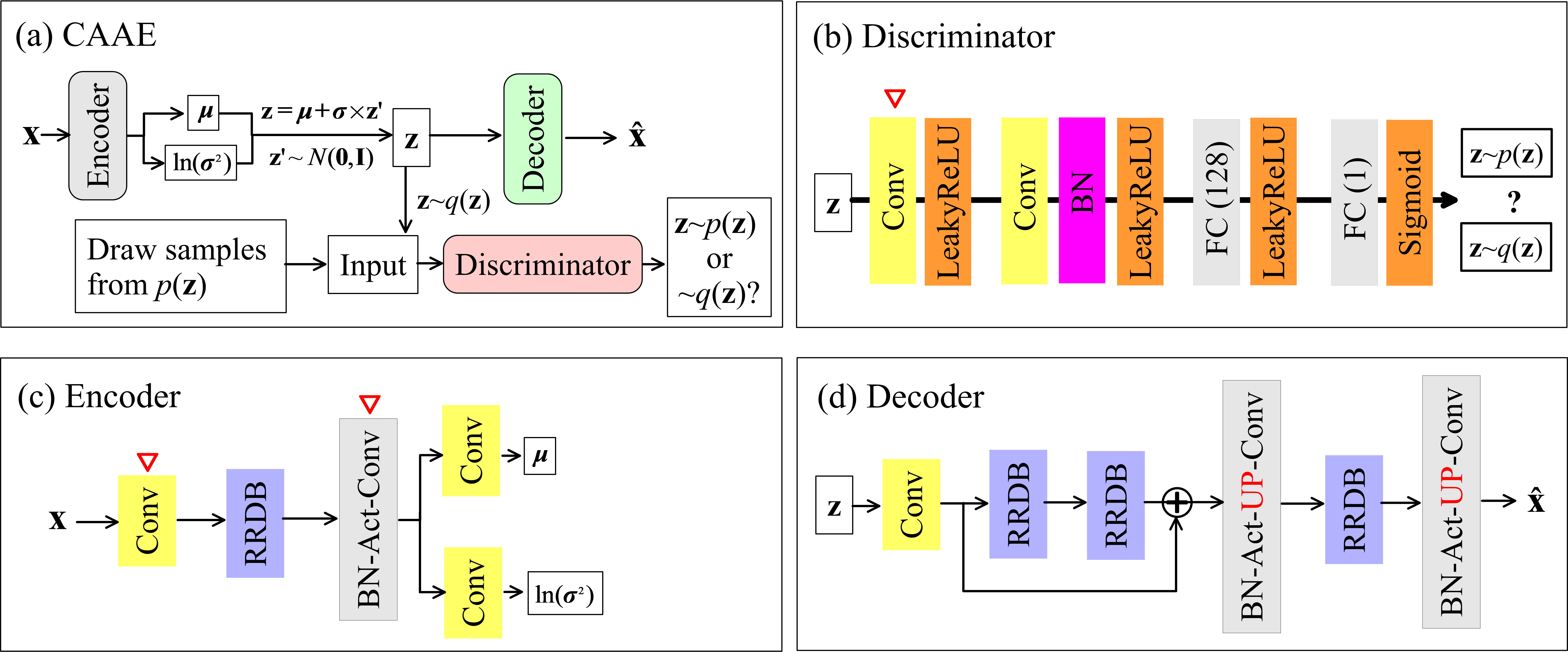 Figure 1
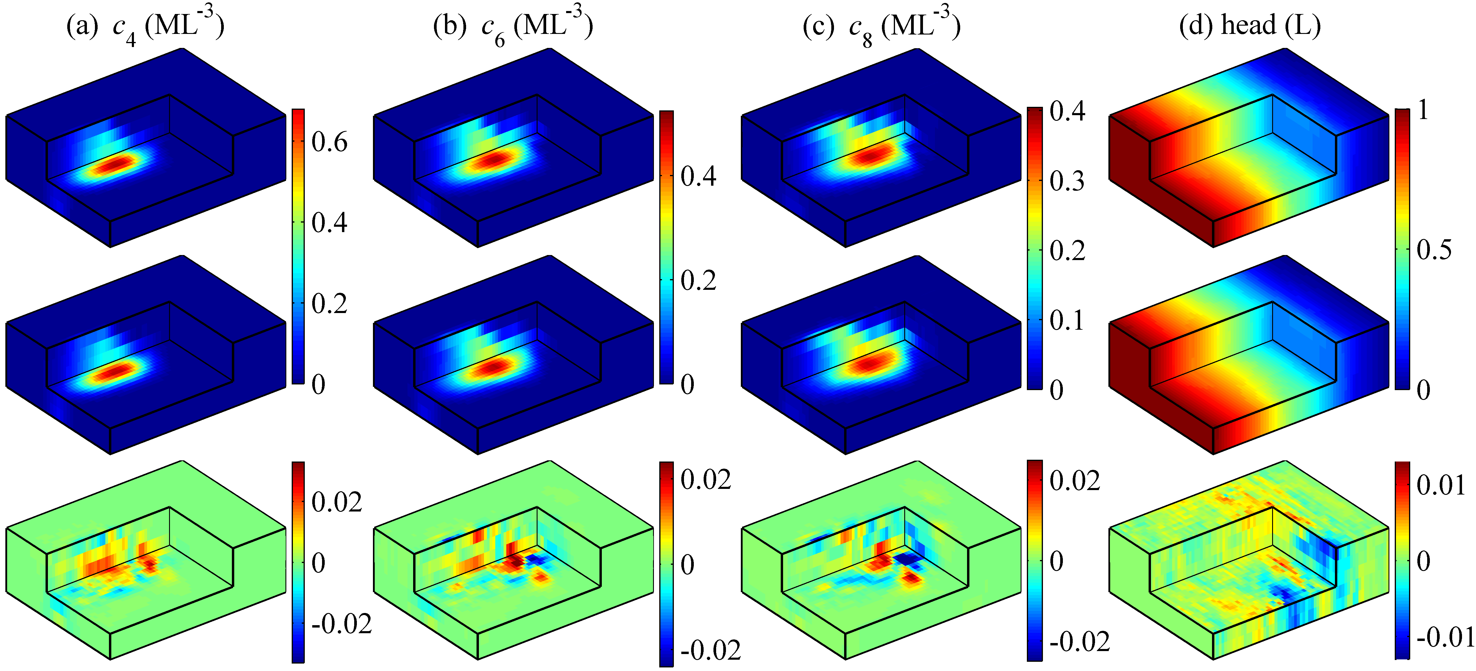 Figure 2
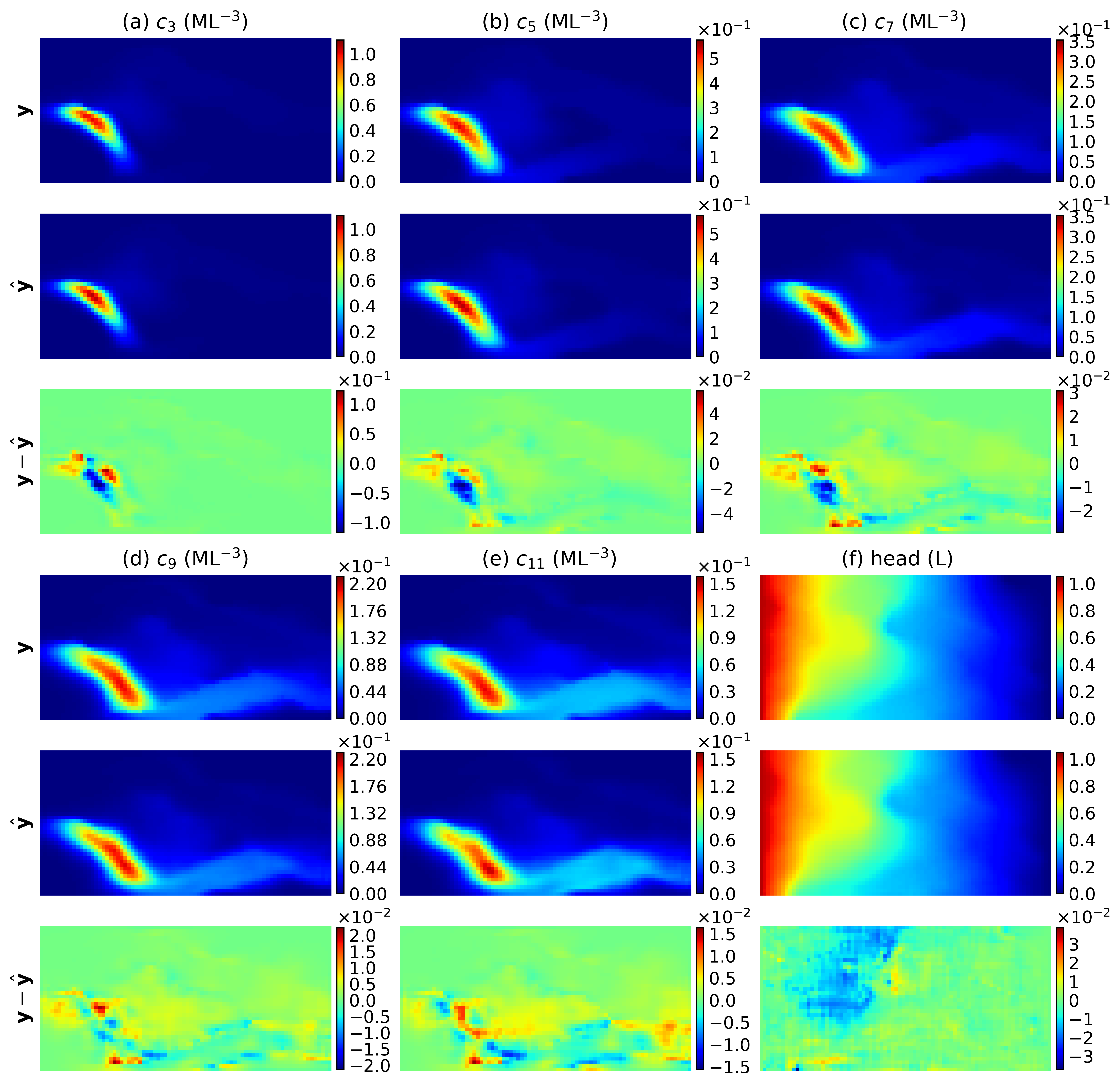 Figure 3
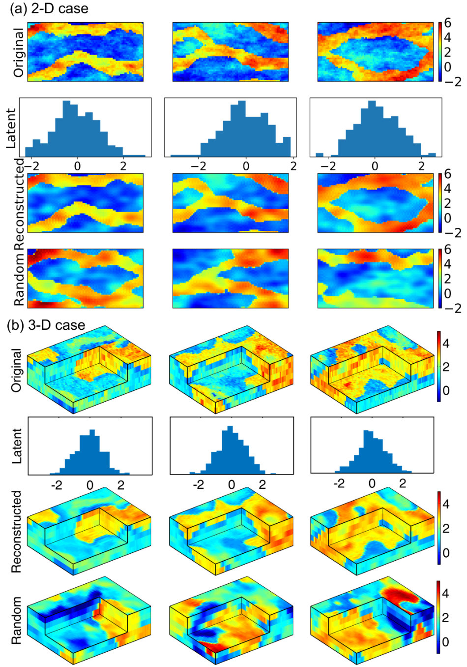 Figure 4
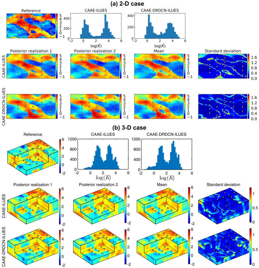 Figure 5
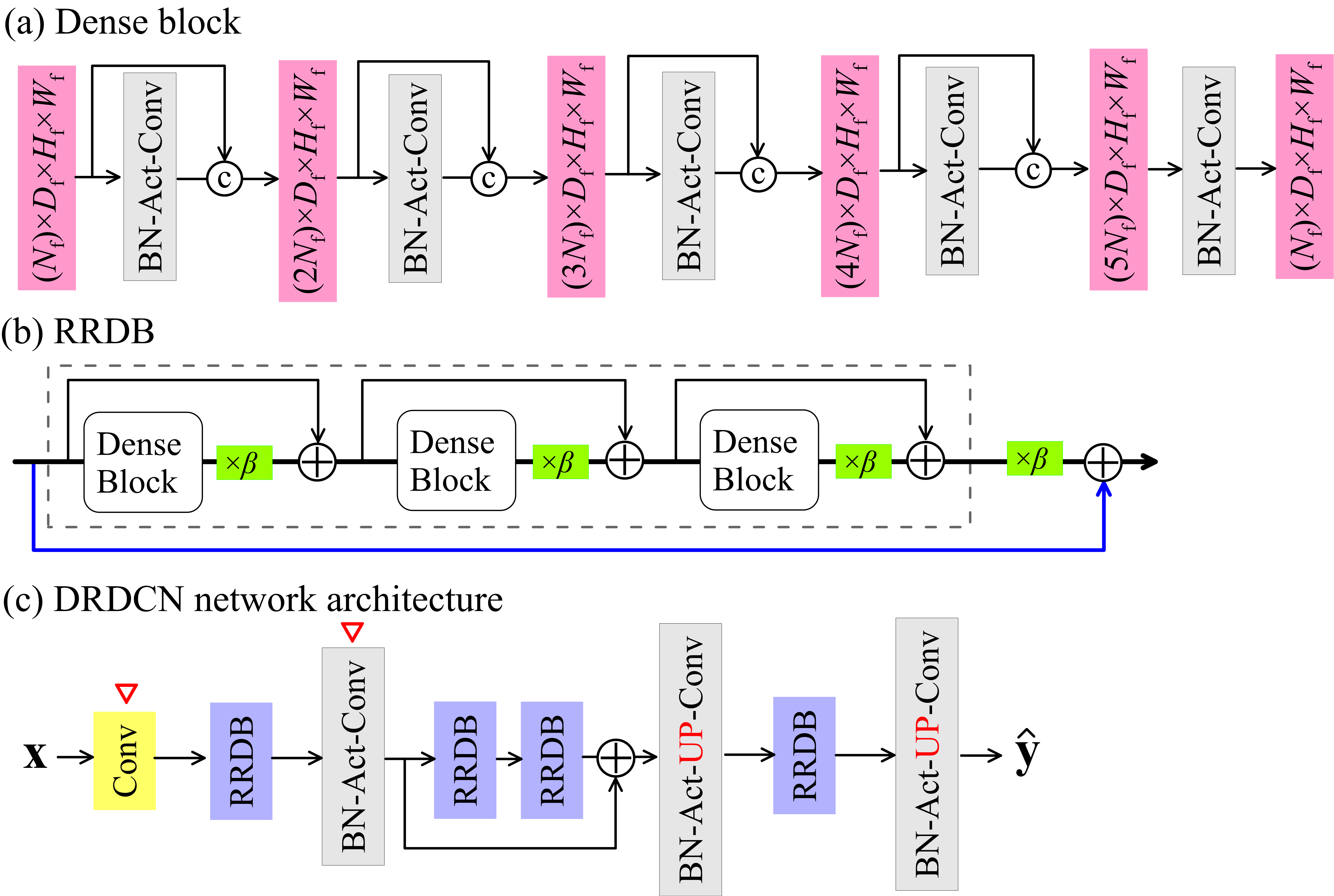 Figure 6
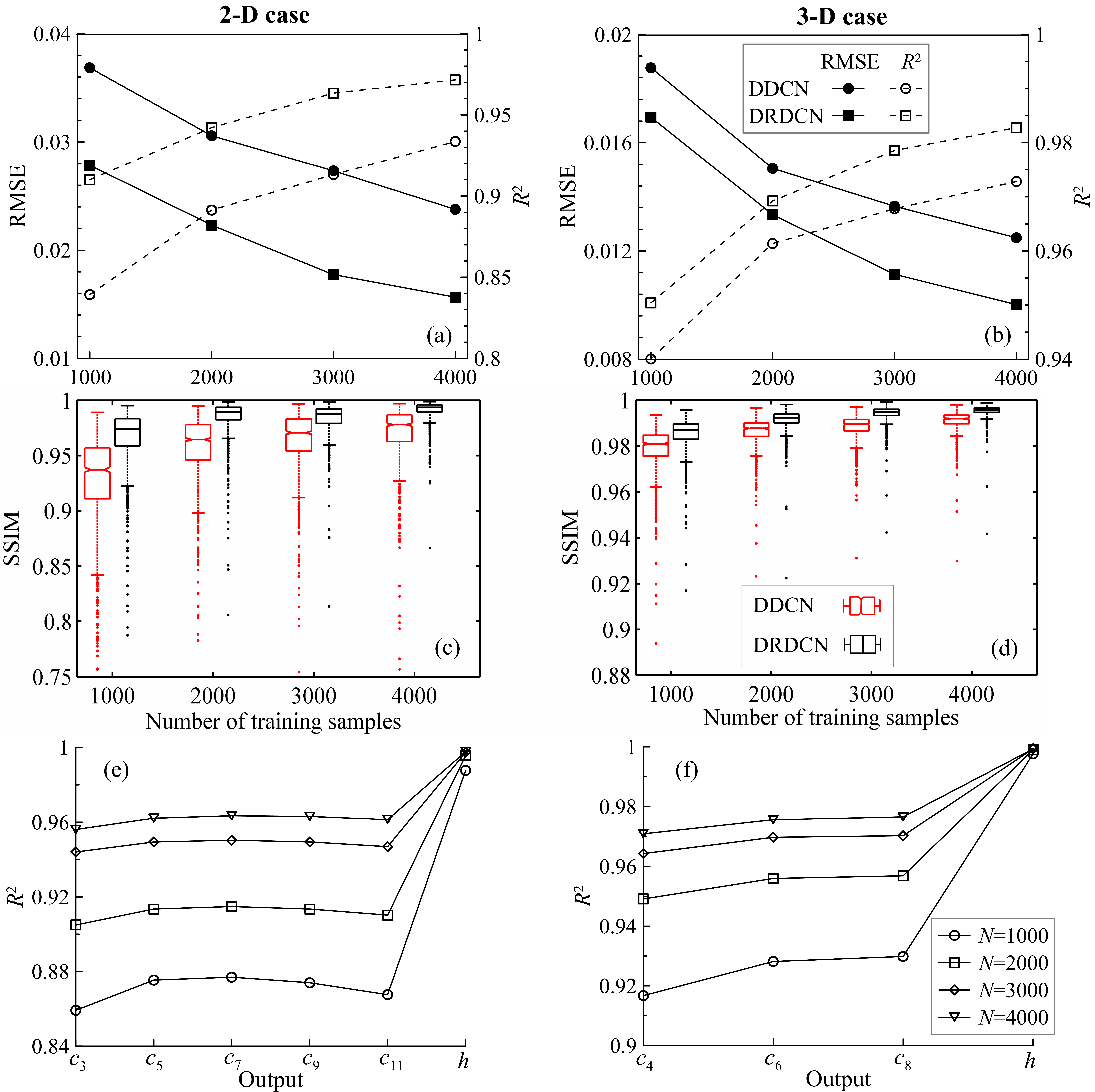 Figure 7
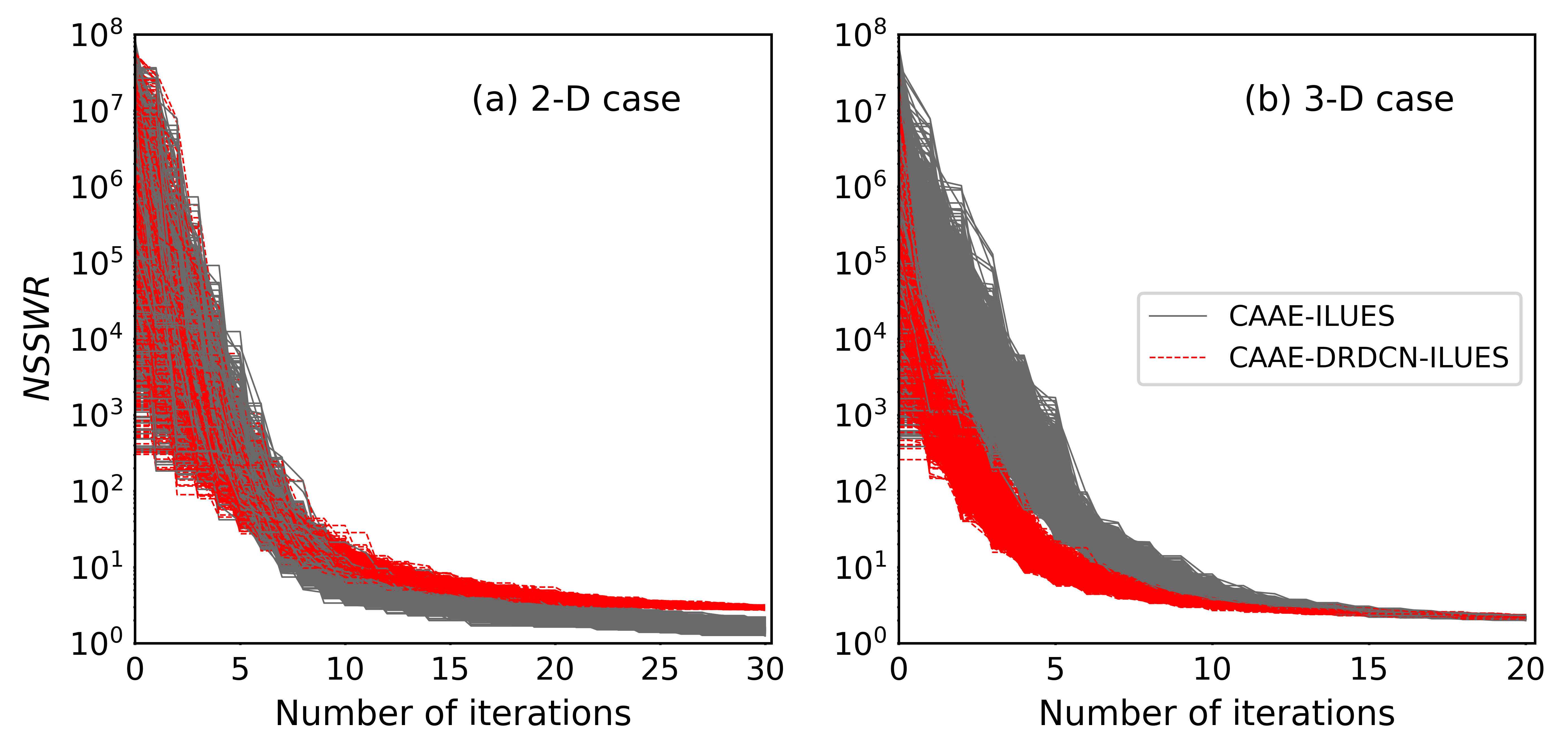 Figure 8
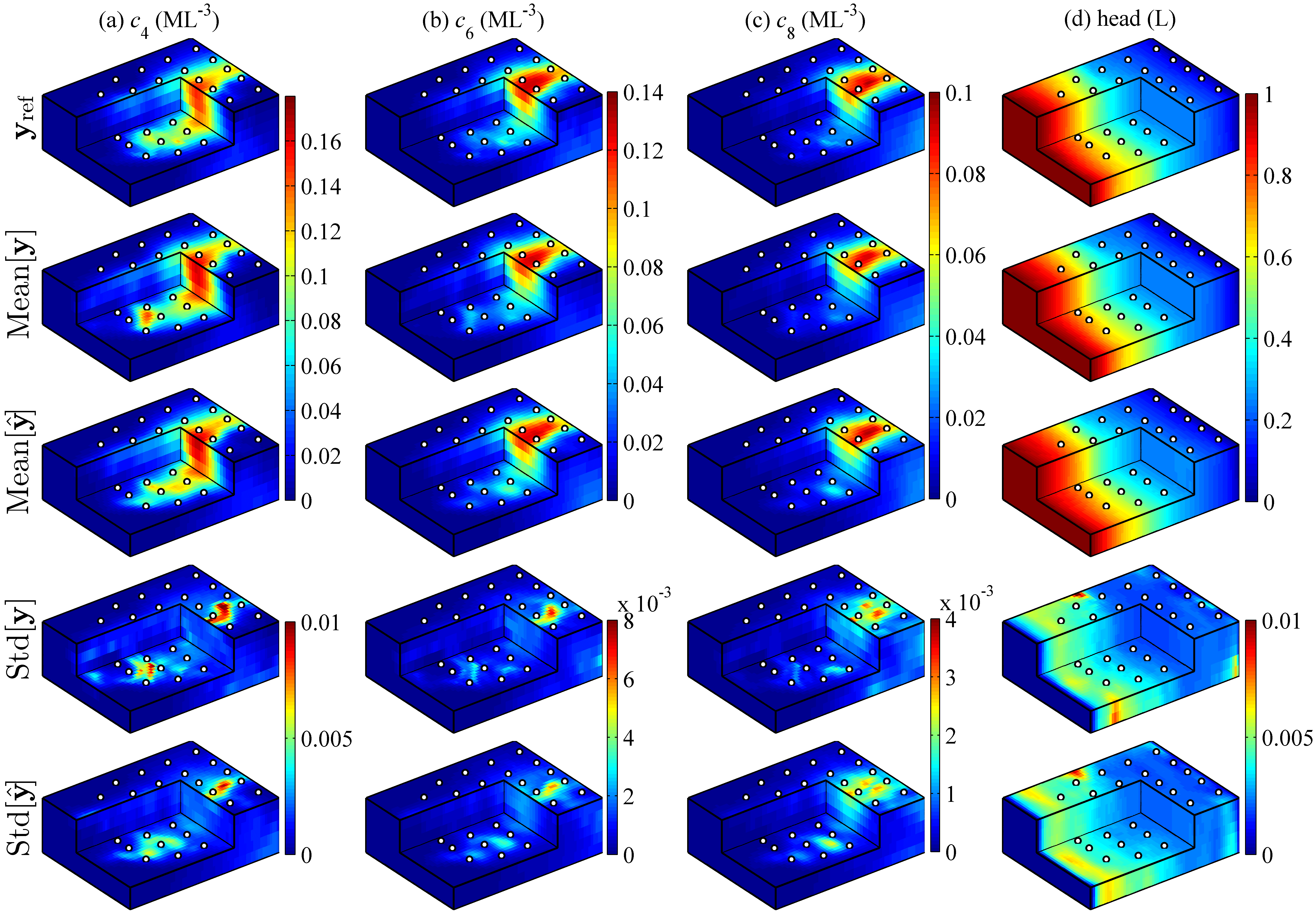 Figure 9
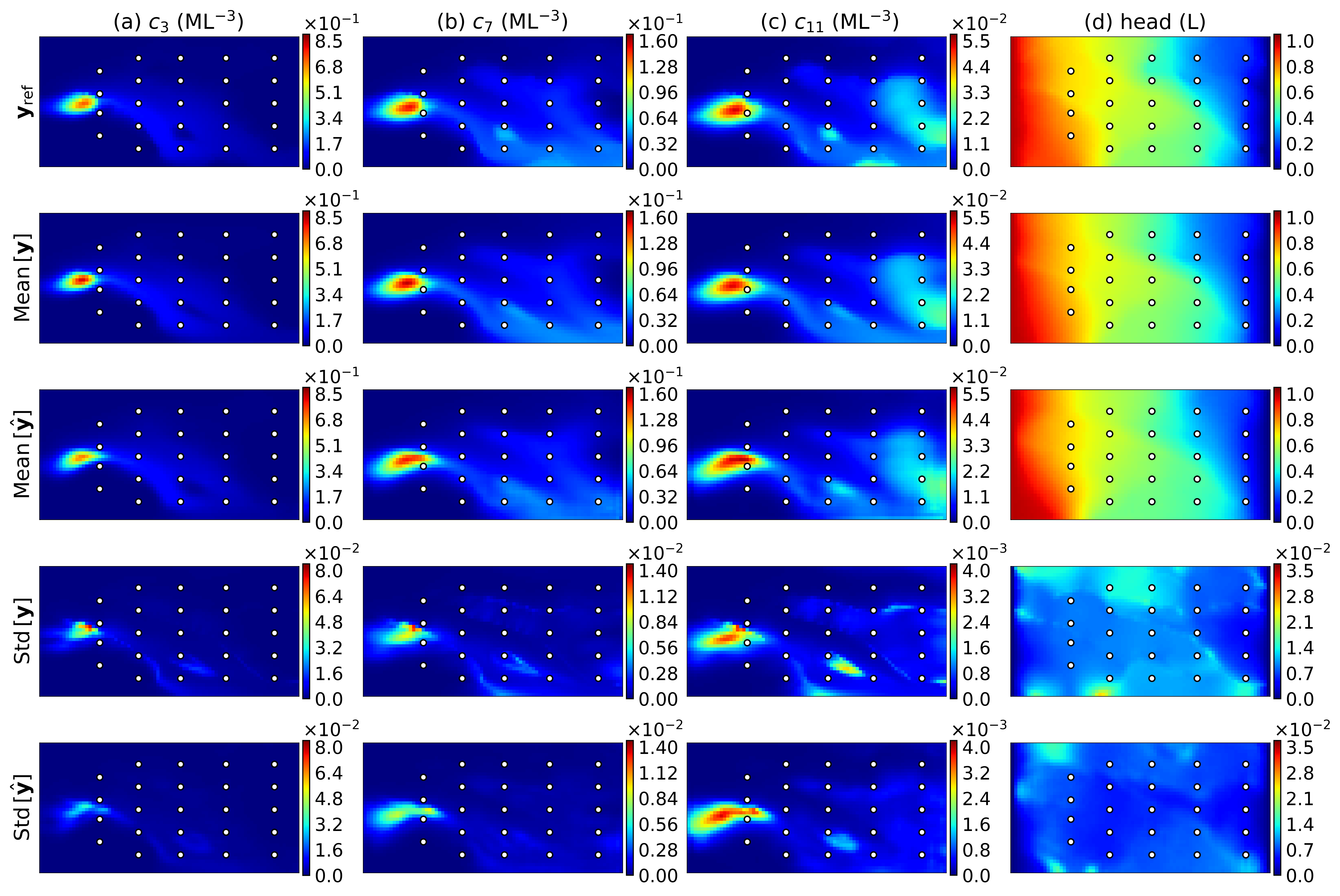 Figure 10
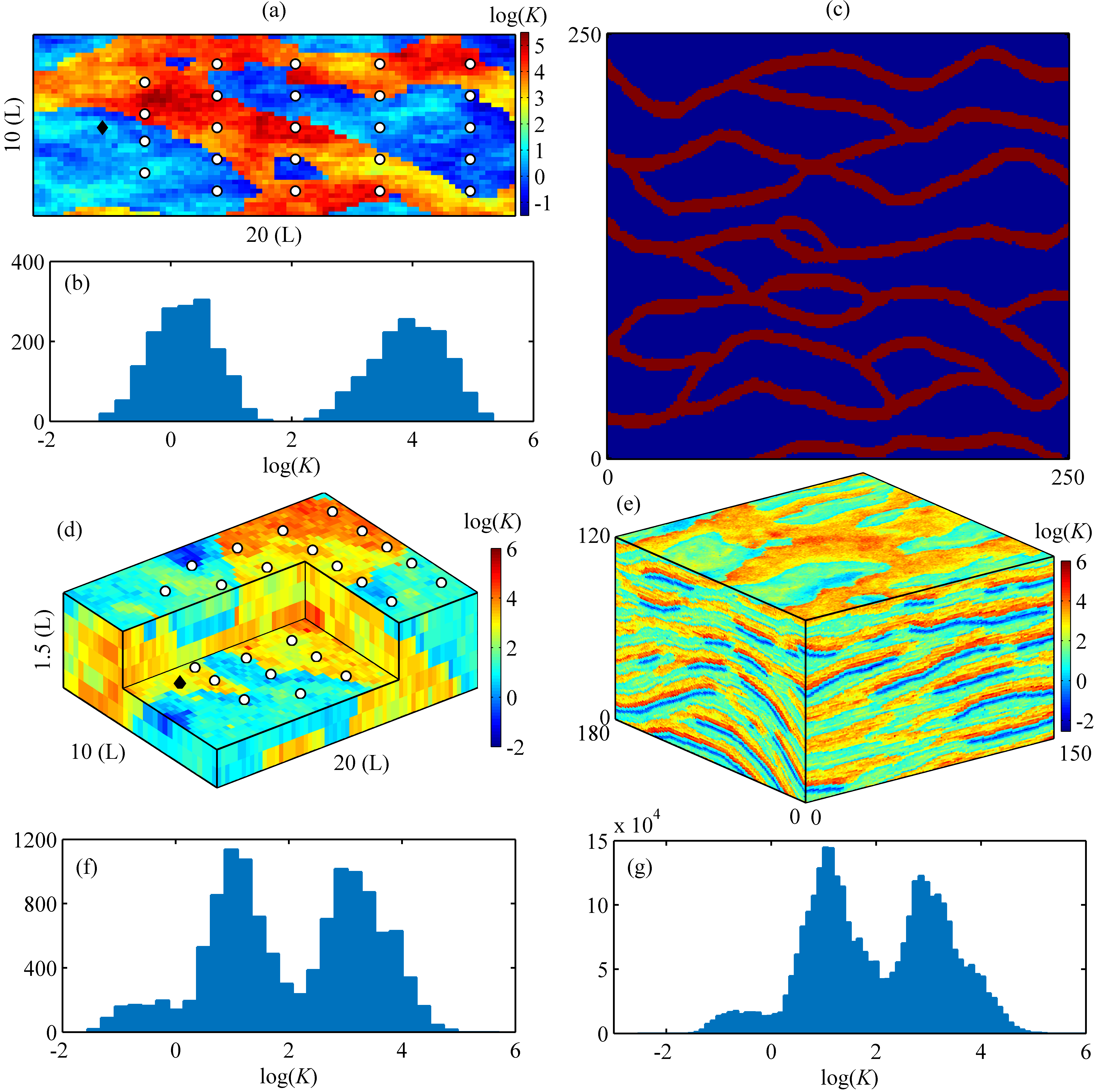 Figure 11
Peer Reviews
No public reviews on file for this paper yet. If you reviewed it on a platform where reviews are public (OpenReview, ICLR, NeurIPS, ICML), you can paste yours below so the community can read it here.
Code & Models
Videos
No videos yet. Explain this paper in a talk, walkthrough, or lecture? Add one.
Taxonomy
Methods(TravEL!!Guide)How Do I File a Claim with Expedia? · Tanh Activation · + ( 1 ) ⟷ 888 ⟷ ( 829 ) ⟷ 0881 How do I file a claim with Expedia? · Solana Customer Service Number +1-833-534-1729
Integration of adversarial autoencoders with residual dense convolutional networks for estimation of non-Gaussian hydraulic conductivities
Abstract
Inverse modeling for the estimation of non-Gaussian hydraulic conductivity fields in subsurface flow and solute transport models remains a challenging problem. This is mainly due to the non-Gaussian property, the non-linear physics, and the fact that many repeated evaluations of the forward model are often required. In this study, we develop a convolutional adversarial autoencoder (CAAE) to parameterize non-Gaussian conductivity fields with heterogeneous conductivity within each facies using a low-dimensional latent representation. In addition, a deep residual dense convolutional network (DRDCN) is proposed for surrogate modeling of forward models with high-dimensional and highly-complex mappings. The two networks are both based on a multilevel residual learning architecture called residual-in-residual dense block. The multilevel residual learning strategy and the dense connection structure ease the training of deep networks, enabling us to efficiently build deeper networks that have an essentially increased capacity for approximating mappings of very high-complexity. The CCAE and DRDCN networks are incorporated into an iterative ensemble smoother to formulate an inversion framework. The numerical experiments performed using 2-D and 3-D solute transport models illustrate the performance of the integrated method. The obtained results indicate that the CAAE is a robust parameterization method for non-Gaussian conductivity fields with different heterogeneity patterns. The DRDCN is able to obtain accurate approximations of the forward models with high-dimensional and highly-complex mappings using relatively limited training data. The CAAE and DRDCN methods together significantly reduce the computation time required to achieve accurate inversion results.
\draftfalse\journalname
Water Resources Research
\justify
Key Laboratory of Surficial Geochemistry of Ministry of Education, School of Earth Sciences and Engineering, Nanjing University, Nanjing, China.
Center for Informatics and Computational Science, University of Notre Dame, Notre Dame, IN, USA.
\correspondingauthor
Nicholas [email protected] \correspondingauthorXiaoqing [email protected]
{keypoints}
A convolutional adversarial autoencoder is developed to parameterize non-Gaussian conductivity fields with multimodal distributions
A deep residual dense convolutional network is introduced as a surrogate of the forward physics-based model
The integrated method is tested with inverse problems for the estimation of non-Gaussian conductivities in solute transport modeling
1 Introduction
Groundwater flow and solute transport models are used widely to help understand subsurface processes and make science-informed decisions for groundwater resource management. Reliable model predictions that well reproduce the phenomena of interest require a good characterization of the hydraulic conductivity field as it greatly influences groundwater flow and solute transport. In many practical cases, such as aquifers in fluvial deposits where several highly contrasting facies coexist, it may be unrealistic to model the log-conductivity as a multivariate Gaussian. It has been shown that a multimodal distribution can better characterize the connectivity between different facies and the multimodality in highly heterogeneous conductivity fields Gómez-Hernández \BBA Wen (\APACyear1998); Journel \BBA Deutsch (\APACyear1993); Kerrou \BOthers. (\APACyear2008); Zhou \BOthers. (\APACyear2014).
In this study, we are concerned with an inverse estimation of non-Gaussian conductivity fields with heterogeneous conductivity within each facies using hydraulic head and solute concentration data. This is in contrast to categorical fields with homogeneous conductivity within each facies (e.g., the binary field) Winter \BOthers. (\APACyear2003), although they both have multimodal distributions. In practice, the conductivity field is estimated via inverse modeling. Commonly used inverse methods are, for example, Markov chain Monte Carlo methods Vrugt (\APACyear2016) and the ensemble-based data assimilation methods such as ensemble smoother van Leeuwen \BBA Evensen (\APACyear1996), ensemble Kalman filter Evensen (\APACyear1994), and their variants Emerick \BBA Reynolds (\APACyear2013); Laloy \BOthers. (\APACyear2013); Sun \BOthers. (\APACyear2009); Xu \BBA Gómez-Hernández (\APACyear2018); J. Zhang \BOthers. (\APACyear2018); Zhou \BOthers. (\APACyear2011). Considering the strong conductivity heterogeneity, the inverse problem is usually high-dimensional. Thus, it often requires a large number of forward model runs to obtain converged inversion results.
To relieve the large computational cost, parameterization methods are commonly used together with surrogate models within the inversion framework. A parameterization method aims to represent the spatially correlated property field using a low-dimensional latent vector Linde \BOthers. (\APACyear2015); Oliver \BBA Chen (\APACyear2011); Zhou \BOthers. (\APACyear2014). It can also 1) mitigate the potential ill-posedness of the inverse problem, 2) ensure that the updated fields in the inversion process satisfy the prior distribution assumptions (e.g., non-Gaussian) imposed on the unknown field, and 3) produce normally distributed latent variables, allowing direct use of second-order inverse methods (e.g., ensemble smoother and ensemble Kalman filter), although these may be at the cost of increased nonlinearity for the inverse problems Laloy \BOthers. (\APACyear2019). In previous studies involving the estimation of non-Gaussian conductivity fields, as noted in the review by \citeALINDE201586, one popular solution is to utilize multiple-point statistics (MPS) simulation in the inversion to generate conductivity field realizations that honor the non-Gaussian prior determined by a training image Hansen \BOthers. (\APACyear2012); Laloy \BOthers. (\APACyear2016); Mariethoz \BOthers. (\APACyear2010); Zahner \BOthers. (\APACyear2016). While such MPS-based inverse methods can generally provide reliable estimations, they may be computationally intensive Laloy \BOthers. (\APACyear2018). A surrogate method aims to replace the computationally expensive forward model with an accurate but cheap-to-run surrogate model during the inversion Asher \BOthers. (\APACyear2015); Razavi \BOthers. (\APACyear2012). Although such combinations of methods for inverse modeling have been intensively studied for problems with Gaussian conductivity fields Chang \BOthers. (\APACyear2017); Elsheikh \BOthers. (\APACyear2014); Ju \BOthers. (\APACyear2018); Laloy \BOthers. (\APACyear2013); J. Zhang \BOthers. (\APACyear2015, \APACyear2016), previous studies on problems with non-Gaussian conductivity fields often relied on the inverse methods solely without using the parameterization and surrogate methods. The development of parameterization and surrogate methods for such non-Gaussian problems remains an open problem due to two major challenges.
First, most existing parameterization methods fail to work for non-Gaussian conductivity fields. Previous works on parameterizing the conductivity fields in inversion has relied on, for example, principal component analysis and its variants Ma \BBA Zabaras (\APACyear2011); Sarma \BOthers. (\APACyear2008); Vo \BBA Durlofsky (\APACyear2014); D. Zhang \BBA Lu (\APACyear2004). While these methods are well suited for Gaussian random fields, their performance for complex non-Gaussian fields deserves further improvement Canchumuni \BOthers. (\APACyear2019\APACexlab\BCnt2); Chan \BBA Elsheikh (\APACyear2017); Laloy \BOthers. (\APACyear2017); Y. Liu \BOthers. (\APACyear2019). Inspired by the recent success of deep learning in various areas including Earth science Bergen \BOthers. (\APACyear2019); Reichstein \BOthers. (\APACyear2019); Zuo \BOthers. (\APACyear2019) and hydrology Shen (\APACyear2018), its application in parameterization of non-Gaussian conductivity fields has been reported in many recent studies Canchumuni \BOthers. (\APACyear2019\APACexlab\BCnt1, \APACyear2019\APACexlab\BCnt2); Chan \BBA Elsheikh (\APACyear2017, \APACyear2018, \APACyear2019); Laloy \BOthers. (\APACyear2017, \APACyear2018); Y. Liu \BOthers. (\APACyear2019). Among these applications, generative adversarial network (GAN) Goodfellow \BOthers. (\APACyear2014) and variational antoencoder (VAE) Kingma \BBA Welling (\APACyear2014) are the two most popular network architectures. After training the network, these methods take random realizations of a low-dimensional vector as input and then generate new realizations of the conductivity field having similar features with those found in the training data. The quality of the generated realizations was shown to be superior to those from traditional parameterization methods Canchumuni \BOthers. (\APACyear2019\APACexlab\BCnt2); Chan \BBA Elsheikh (\APACyear2017); Laloy \BOthers. (\APACyear2017); Y. Liu \BOthers. (\APACyear2019). However, these methods focused on categorical conductivity fields with homogeneous conductivity within each facies. Their applicability to non-Gaussian fields with heterogeneous conductivity within each facies, which is more challenging, remains to be further investigated. \citeAlaloy2018 and \citeALiu2019 further tested their methods’ potential for such continuous fields. While the results suggested a promising performance of the deep learning-based parameterization methods, no inversion results were presented. \citeACanchumuni201987 considered channelized conductivity fields with a bimodal distribution. They used a VAE network to generate binary channelized fields and the uncertain parameters to be estimated in the inversion are the latent variables and the permeability values at all grid points, with the inverse problem remaining high-dimensional.
Second, most existing surrogate methods suffer from the curse of dimensionality Asher \BOthers. (\APACyear2015); Razavi \BOthers. (\APACyear2012) and fail to efficiently obtain accurate approximations when the input-output relations are highly-nonlinear Liao \BOthers. (\APACyear2017); Lin \BBA Tartakovsky (\APACyear2009); Mo \BOthers. (\APACyear2017). The curse of dimensionality is caused by the exponentially increased computational cost required for accurate surrogate construction as the input dimensionality (i.e., the number of uncertain variables considered) increases. Due to the strongly heterogeneous nature of the conductivity field, it is often required to use a large number of stochastic degrees of freedom to accurately represent the heterogeneity. The highly-nonlinear outputs here arise because the high-conductivity regions in a non-Gaussian aquifer result in preferential paths for the groundwater flow and solute transport. The two factors together make the commonly used surrogate methods, such as Gaussian processes Rasmussen \BBA Williams (\APACyear2006) and polynomial chaos expansion Xiu \BBA Karniadakis (\APACyear2002), difficult to work. Deep neural networks have already exhibited a promising and impressive performance for surrogate modeling of forward models with high-dimensional input and output fields Kani \BBA Elsheikh (\APACyear2019); Mo, Zabaras\BCBL \BOthers. (\APACyear2019); Mo, Zhu\BCBL \BOthers. (\APACyear2019); Sun (\APACyear2018); Tripathy \BBA Bilionis (\APACyear2018); Zhong \BOthers. (\APACyear2019); Zhu \BBA Zabaras (\APACyear2018); Zhu \BOthers. (\APACyear2019). For example, in \citeATripathy2018 a deep neural network was proposed to build a surrogate model for a single-phase flow forward model. In \citeASun2018 and \citeAZhong2019, their surrogate methods for a single-phase flow forward model and a multiphase flow forward model, respectively, were based on an adversarial network framework. In our previous studies Mo, Zabaras\BCBL \BOthers. (\APACyear2019); Mo, Zhu\BCBL \BOthers. (\APACyear2019); Zhu \BBA Zabaras (\APACyear2018); Zhu \BOthers. (\APACyear2019), a deep dense convolutional network (DDCN), which is based on a dense connection structure Huang \BOthers. (\APACyear2017) for better information flow efficiency, was employed as the surrogate modeling framework. It showed a good performance in efficiently obtaining accurate surrogates of various forward models with high-dimensional input-output mappings. However, these methods were tested on forward models with Gaussian conductivity fields Kani \BBA Elsheikh (\APACyear2019); Mo, Zabaras\BCBL \BOthers. (\APACyear2019); Mo, Zhu\BCBL \BOthers. (\APACyear2019); Tripathy \BBA Bilionis (\APACyear2018); Zhu \BBA Zabaras (\APACyear2018); Zhu \BOthers. (\APACyear2019) or on a single-phase flow model with binary channelized conductivity fields Zhu \BOthers. (\APACyear2019). As shown in a case study below, the application of the DDCN surrogate method to solute transport modeling with non-Gaussian conductivity fields may lead to large approximation errors.
In this work, we develop a convolutional adversarial autoencoder (CAAE) to parameterize non-Gaussian conductivity fields with multimodal distributions. We transform a fully-connected adversarial autoencoder Makhzani \BOthers. (\APACyear2016) to a convolutional network so as to improve its scalability for larger-size inputs. In addition, we propose a deep residual dense convolutional network (DRDCN) for efficient surrogate modeling of forward models with high-dimensional and highly-complex mappings. Although deeper networks have the potential to substantially improve the network’s performance, they can be difficult to train. We adopt in DRDCN a multilevel residual learning structure X. Wang \BOthers. (\APACyear2018). The residual learning strategy has been shown to be an effective solution to ease the training of very deep networks He \BOthers. (\APACyear2016\APACexlab\BCnt1, \APACyear2016\APACexlab\BCnt2); Simonyan \BBA Zisserman (\APACyear2015); Szegedy \BOthers. (\APACyear2015); X. Wang \BOthers. (\APACyear2018). The multilevel residual learning structure is also implemented in the CAAE network. The CAAE and DRDCN networks are combined with an iterative local updating ensemble smoother (ILUES) algorithm J. Zhang \BOthers. (\APACyear2018) to formulate an efficient CAAE-DRDCN-ILUES inversion framework. The overall integrated method is demonstrated using 2-D and 3-D solute transport modeling with non-Gaussian conductivity fields that have different heterogeneity patterns.
In summary, three major innovative contributions are addressed in this study. First, we develop a CAAE method for parameterization of non-Gaussian conductivity fields with heterogeneous conductivity within each facies that is suitable in the context of inverse modeling. Second, we adopt a multilevel residual strategy in our previous DDCN method Mo, Zabaras\BCBL \BOthers. (\APACyear2019); Mo, Zhu\BCBL \BOthers. (\APACyear2019); Zhu \BBA Zabaras (\APACyear2018); Zhu \BOthers. (\APACyear2019) to introduce a new DRDCN method with a substantially improved performance for surrogate modeling of highly-complex mappings. Finally and most importantly, to the best of our knowledge, we present the first attempt to incorporate simultaneously the parameterization and surrogate methods to perform inversion for non-Gaussian conductivities in solute transport modeling.
The rest of the paper is organized as follows. In section 2, we introduce a solute transport model and define the problem of interest. The CAAE-DRDCN-ILUES inversion framework is presented in section 3. Then in sections 4 and 5, the proposed method is evaluated using two synthetic examples. The conclusions are summarized in the last section.
2 Problem Definition
We consider solute transport in heterogeneous porous media under a steady-state groundwater flow condition. It is assumed that the transport of solute is driven by advection and dispersion. The governing equations for the steady-state flow and solute transport are written as Zheng \BBA Wang (\APACyear1999)
[TABLE]
and
[TABLE]
respectively. Here (LT*-1*) is the hydraulic conductivity, (L) is the hydraulic head, (-) is the effective porosity, (ML*-3*) is the solute concentration, (T) denotes time, (ML*-3T-1*) is the sink/source, and (L2T*-1*) is the dispersion tensor determined by the pore space flow velocity (LT*-1*), and longitudinal (; L), transverse (; L), and vertical (; L) dispersivities. The two equations are coupled through the velocity . The flow and solute transport equations are numerically solved using the MODFLOW Harbaugh \BOthers. (\APACyear2000) and MT3DMS Zheng \BBA Wang (\APACyear1999) simulators, respectively.
We are concerned with an inverse problem of characterizing the heterogeneous conductivity field using measurements of the hydraulic head and concentration. The underlying conductivity fields of interest are non-Gaussian fields with a multimodal distribution. The inverse modeling is performed using the ILUES inversion algorithm J. Zhang \BOthers. (\APACyear2018) which has shown a promising performance for high-dimensional and highly-nonlinear inverse problems Mo, Zabaras\BCBL \BOthers. (\APACyear2019); J. Zhang \BOthers. (\APACyear2018).
3 Methodology
3.1 ILUES for Inverse Modeling
The ILUES algorithm assimilates the output measurements for multiple times with an inflated covariance matrix of the measurement errors to avoid overweighing the measurements J. Zhang \BOthers. (\APACyear2018). The inflated covariance matrix is often taken as , where is the original covariance matrix of the measurement errors and is the number of iterations Emerick \BBA Reynolds (\APACyear2013); J. Zhang \BOthers. (\APACyear2018). To better handle high-dimensional and highly-nonlinear problems, ILUES also adopts a local updating scheme, which updates each input sample (in the CAAE-DRDCN-ILUES framework, refers to the latent variables, see section 3.4) in the ensemble locally using its neighboring samples rather than all samples in the ensemble. Formally, given an ensemble of input samples , it first identifies a local ensemble for each sample based on the following metric J. Zhang \BOthers. (\APACyear2018)
[TABLE]
where quantifies the mismatch between the model responses and measurements , and is the distance between the sample and . Here, is the autocovariance matrix of the input parameters in , and are the maximum values of and , respectively. Based on the values, we select samples as the local ensemble of using a roulette wheel selection operator Lipowski \BBA Lipowska (\APACyear2012), in which the selection probability of the th individual is given as , , where Mo, Zabaras\BCBL \BOthers. (\APACyear2019). A local ensemble factor of suggested in \citeAzhang2018ILUES is used.
Let superscripts , , and denote the local ensemble, current and updated samples, respectively. The ILUES first updates the local ensemble of each sample , that is, , by using the usual ensemble smoother scheme Emerick \BBA Reynolds (\APACyear2013); J. Zhang \BOthers. (\APACyear2018):
[TABLE]
for . Here is the cross-covariance matrix between and \mathbf{D}_{i}^{l,f}=\big{[}f(\bm{m}_{i,1}^{f}),\ldots,f(\bm{m}_{i,N_{l}}^{f})\big{]}, is the autocovariance matrix of , and , , is the -th realization of the measurements. The update of , , is then generated from its updated local ensemble through a probabilistic scheme Mo, Zabaras\BCBL \BOthers. (\APACyear2019). One update iteration of ILUES is summarized in Algorithm 1. More details regarding ILUES can be found in \citeAzhang2018ILUES and \citeAmo2019inverse.
For high-dimensional inverse problems, large ensemble size and iteration number are usually needed for ILUES to obtain converged and reliable inversion results, resulting in a large computational cost in forward model runs. To reduce the computational burden, we propose a CAAE network for parameterizing the high-dimensional conductivity field using a low-dimensional latent vector and a DRDCN network to build an accurate but fast-to-run substitution of the forward model in the ILUES algorithm.
3.2 DRDCN for Surrogate Modeling
In the surrogate modeling task, we build a surrogate model to approximate the mapping between the input conductivity field and the output hydraulic head and concentration fields. In our previous studies Mo, Zabaras\BCBL \BOthers. (\APACyear2019); Mo, Zhu\BCBL \BOthers. (\APACyear2019); Zhu \BBA Zabaras (\APACyear2018); Zhu \BOthers. (\APACyear2019), we transformed the surrogate modeling task for problems with high-dimensional input and output fields in a 2-D domain to an image-to-image regression problem by using a DDCN network. In this network, the input and output fields were treated as images. Denoting as the spatial discretization resolution of the domain, and as the input and output fields, respectively. Then the surrogate modeling task for approximating the input-output mapping,
[TABLE]
was transformed to an image regression problem between input images and output images with a resolution of , where and are the number of the input and output fields, respectively. It is straightforward to generalize to a 3-D domain by adding an extra depth axis to the images, that is, .
In order to further improve the performance of DDCN in problems with highly-complex mappings, we adopt a novel basic block called ‘residual-in-residual dense block’ proposed in \citeAWang-etal2018 for image super-resolution problems to formulate our DRDCN framework.
3.2.1 Residual-in-Residual Dense Block
A dense block introduces connections between non-adjacent layers aiming to fully exploit the hierarchical features from the outputs of preceding layers Huang \BOthers. (\APACyear2017). Let () denote the output feature maps of the th layer in the dense block, where is number of layers. is obtained by taking the concatenation of the output feature maps from its preceding layers as input, as represented by
[TABLE]
where represents the input to the dense block, and denotes operations on the input feature maps, including batch normalization (BN) Ioffe \BBA Szegedy (\APACyear2015), followed by nonlinear activation and convolution (Conv) Goodfellow \BOthers. (\APACyear2016). The ReLU (Rectified Linear Unit) function defined as is commonly used. Alternatively, a new activation function Mish Misra (\APACyear2019), which is defined as , can be used. It has been shown to perform generally better than ReLU in many deep networks across many datasets Misra (\APACyear2019). A dense block with layers is illustrated in Figure 1a.
It has been shown that deeper networks have the potential to better approximate mappings of high complexity, however, they can be difficult to train Simonyan \BBA Zisserman (\APACyear2015); Szegedy \BOthers. (\APACyear2015); X. Wang \BOthers. (\APACyear2018). To efficiently train a deeper network, we adopt a multilevel residual learning structure, that is, the residual-in-residual dense block proposed in \citeAWang-etal2018. In the residual learning framework, it has been shown that the residual mapping is much easier to learn than the original mapping He \BOthers. (\APACyear2016\APACexlab\BCnt1, \APACyear2016\APACexlab\BCnt2). Specifically, let denote the desired underlying mapping to fit. Then the stacked layers (not necessarily the entire network) learn the residual mapping . The original mapping is then recast as . Such a residual learning strategy can help alleviate the gradient vanishing problem for deep network training He \BOthers. (\APACyear2016\APACexlab\BCnt1) and thus ease the training of very deep networks to achieve improved accuracy He \BOthers. (\APACyear2016\APACexlab\BCnt1, \APACyear2016\APACexlab\BCnt2); Ledig \BOthers. (\APACyear2017); Simonyan \BBA Zisserman (\APACyear2015); X. Wang \BOthers. (\APACyear2018).
The architecture of residual-in-residual dense block is shown in Figure 1b. It consists of a stack of residual dense blocks, where the residual learning is used in two levels, resulting in a residual-in-residual structure. That is, the residual learning implemented to the dense block results in a residual dense block; and that implemented to the stacked residual dense blocks results in a residual-in-residual dense block. The number of input and output feature maps of a dense block is (Figure 1a) and is set to . In addition to the residual-in-residual structure, a residual scaling technique Szegedy \BOthers. (\APACyear2016) is also employed in the residual-in-residual dense block to further increase the training stability X. Wang \BOthers. (\APACyear2018). Formally, this is done by scaling down the residual by a factor before adding to (Figure 1b). A factor of suggested in \citeAWang-etal2018 is used in our network.
3.2.2 DRDCN Networks Based on Residual-in-Residual Dense Blocks
We employ the residual-in-residual dense block structure in our DRDCN network for surrogate modeling of solute transport in media with non-Gaussian conductivities. The network architecture is shown in Figure 1c. For 2-D or 3-D images (fields), the 2-D and 3-D operations (i.e., BN and Conv) implemented in the PyTorch software are respectively used in the network. The network contains four residual-in-residual dense blocks and the feature maps are to go through a coarsen-to-refine process. A convolutional layer is first employed to extract feature maps from the raw input image. The obtained features are then passed through the residual-in-residual dense blocks and the transition convolutional layers for downsampling/upsampling of the feature maps. We arrange the position of the four residual-in-residual dense blocks in the network with a layout of (Figure 1c) to encourage the information flow through the coarse feature maps. That is, one block is placed in the coarsening part; two adjacent blocks are placed in the most central part; and another one block is placed in the refining part. An additional level of residual learning is implemented to the stacked residual-in-residual dense blocks, resulting in a three-level residual learning structure in the network. In DRDCN, the Mish activation is used unless otherwise stated.
3.3 CAAE for Parameterization of Non-Gaussian Random Fields
We propose to parameterize non-Gaussian conductivity fields with multimodal distributions using a CAAE network. Without loss of generality, here we use to denote the log-conductivity field. Adversarial autoencoder is a probabilistic autoencoder that uses the GAN framework as a variational inference algorithm Makhzani \BOthers. (\APACyear2016). The original adversarial autoencoder framework is composed of fully-connected layers Makhzani \BOthers. (\APACyear2016), making it increasingly difficult to train as the network gets deeper due to a large number of trainable parameters. To resolve this issue, we develop a CAAE framework based on convolutional layers to leverage their sparse-connectivity and parameter-sharing properties as well as robust capability in image-like data processing Goodfellow \BOthers. (\APACyear2016); Laloy \BOthers. (\APACyear2018); Mo, Zhu\BCBL \BOthers. (\APACyear2019); Shen (\APACyear2018).
3.3.1 Generative Adversarial Networks
GAN Goodfellow \BOthers. (\APACyear2014) is a framework that establishes an adversarial game between two networks: a generative network (i.e., generator) that learns the distribution over the data, and a discriminative network (i.e., discriminator) that computes the probability that a sample is sampled from , rather than generated by the generator. The generator maps the low-dimensional latent vector from the prior distribution to the data space. The discriminator is trained to maximize the probability of distinguishing the real samples from the generated (fake) samples. The generator is simultaneously trained to maximally fool the discriminator into assigning a higher probability to the generated samples by leveraging the feedback from the discriminator. Mathematically, the adversarial game translates into the following minimization-maximization loss function Goodfellow \BOthers. (\APACyear2014)
[TABLE]
In practice, the generator and discriminator are usually trained in alternating steps: (1) train the discriminator to improve its discriminative capability; (2) train the generator to improve the quality of the generated samples so as to fool the discriminator.
3.3.2 Adversarial Autoencoder
An autoencoder is a framework that learns a low-dimensional representation (referred to as latent codes or latent variables) of a sample in the data and generates from the codes a reconstruction that closely matches . It consists of two networks: an encoder to learn a mapping from to and a decoder to learn a mapping from to . To create a generative framework, in adversarial autoencoder Makhzani \BOthers. (\APACyear2016) a constraint is added on the encoder that forces it to generate latent codes that roughly follow a desired distribution, like a standard normal distribution used in the present study. The decoder is then trained to generate samples with features being consistent with those found in the training data given any sample as input, resulting in a generative model.
Mathematically, let be the encoding distribution, be the decoding distribution, and be the distribution that we want the latent variables to follow. The adversarial autoencoder looks for a generative model
[TABLE]
The adversarial autoencoder Makhzani \BOthers. (\APACyear2016) is very similar to the VAE Kingma \BBA Welling (\APACyear2014) in the sense that in both a latent representation is obtained with a desired distribution. Thus we follow the formulation in VAE to finally introduce the adversarial autoencoder. In VAE, the generative model is obtained via minimizing the upper-bound of the negative log-likelihood
[TABLE]
The first term on the right side quantifies the reconstruction quality and the second term is the Kullback-Leibler divergence measuring the difference between two distributions.
In adversarial autoencoders, an adversarial training procedure instead of the Kullback-Leibler divergence is used to encourage an aggregated posterior distribution , instead of , to match , where is defined as Makhzani \BOthers. (\APACyear2016)
[TABLE]
An illustration of the adversarial autoencoder is depicted in Figure 2a. In the encoding path, the input is fed into the encoder which outputs two low-dimensional vectors of means and log-variances of the latent variables . Then a vector is randomly drawn from and rescaled to produce the codes , where denotes element-wise multiplication. The decoder takes as input to eventually generate . Meanwhile, the discriminator of the adversarial network accepts input from the latent codes generated by the encoder or the prespecified distribution to discriminatively predict whether the input arises from the encoding codes (fake sample) or (real sample). Note that the adversarial network here differs slightly from the vanilla GAN framework Goodfellow \BOthers. (\APACyear2014), in which the generator generates the sample , and the discriminator discriminates whether it is from the generator or the data.
The encoder (which is also the generator of the adversarial network), decoder, and discriminator of the adversarial autoencoder are trained jointly in two phases for each iteration: the reconstruction phase and the regularization phase Makhzani \BOthers. (\APACyear2016). In the reconstruction phase, the encoder (generator) and decoder are updated using the following loss function:
[TABLE]
where is the reconstruction error which in this study is taken as the loss:
[TABLE]
and measures the generator’s ability to fool the discriminator and has the form
[TABLE]
Here, is a weight factor balancing the two losses and a value of is used, is the reconstruction of sample , and is the number of training samples. In the regularization phase, the discriminator is updated based on the loss function
[TABLE]
to distinguish the real sample from (i.e. ) from the fake sample produced by the generator.
Such adversarial training process with the loss functions defined in equations (11) and (14) forces to closely match and to gradually approach (i.e., and ), respectively. After training, the decoder will define a generative model that given an arbitrary input can generate a new realization of sample with features similar to those in the data used for training (Figure 2d).
3.3.3 CAAE Networks Based on Residual-in-Residual Dense Blocks
We also adopt the residual-in-residual dense block structure shown in Figure 1b in the encoder and decoder of the CAAE network. The encoder (Figure 2c) is similar to the coarsening part of the DRDCN network (Figure 1c). The encoder has two additional convolutional layers to respectively output the means and log-variances . The decoder (Figure 2d) is similar to the refining part of the DRDCN network. The decoder has an additional convolutional layer to extract feature maps from the codes . The ReLU activation is used in the encoder and decoder. Inspired by \citeALedig2017CVPR, the discriminator is a stack of two convolutional layers followed by two fully-connected layers with and neurons, respectively. The leaky ReLU activation with a slope of is used in the discriminator and the sigmoid activation is used in the last layer to output a probability value between [math] and .
3.4 The CAAE-DRDCN-ILUES inversion framework
We incorporate the CAAE parameterization method and the DRDCN surrogate method into ILUES to formulate an efficient inversion scheme for estimation of a non-Gaussian conductivity field of solute transport models. The integrated methodology is denoted as CAAE-DRDCN-ILUES hereinafter and is summarized in Algorithm 2. Notice that in this method, the surrogate model is used in Algorithms 1 and 2 to substitute the forward model. After parameterization, the uncertain parameters to be estimated are the latent variables . The log-conductivity field is estimated with the following procedure: (1) start with an initial latent code ensemble drawn from , (2) the corresponding log-conductivity fields are generated next using the CAAE’s decoder, (3) the surrogate model is evaluated to obtain the predicted initial output ensemble, (4) the latent code and output ensembles are repeatedly updated for iterations using Algorithm 1 based on the current latent code and output ensembles. In Algorithm 1, the input to the surrogate model to produce output predictions is the log-conductivity field, which is generated by the CAAE’s decoder given the latent codes as input. The posterior log-conductivity fields are obtained from the decoder using the last latent code ensemble as input.
4 Application
4.1 Solute Transport Models
The performance of the proposed method is illustrated using 2-D and 3-D solute transport modeling with random conductivity fields that have non-Gaussian heterogeneity patterns.
4.1.1 2-D Model
The first test case considers 2-D solute transport within a channelized aquifer. As shown in Figure 3a, the horizontal domain has a size of and is uniformly discretized into gridblocks. The left and right boundaries are assumed to be constant head boundaries with heads of and , respectively. No-flow boundary condition is imposed on the upper and lower boundaries. An instantaneous source with a concentration of (ML*-3*) is released from the location (L) and (L) at the initial time. The porosity and dispersivities are assumed to be known with constant values of , (L) and (L), respectively.
The non-Gaussian conductivity field in this case has a channelized and bimodal pattern with heterogeneous conductivity within each facies. The conductivity realizations are generated by the following procedure: First, a binary facies field is generated using the SNESIM code Strebelle (\APACyear2002) with a training image shown in Figure 3c; then we populate each facies with log-conductivity values from two independently generated Gaussian random fields with a norm exponential covariance function:
[TABLE]
where and denote two arbitrary spatial locations, is the variance, and and are the correlation lengths along the and axes, respectively. The means of Gaussian random fields corresponding to the high-conductivity channels and the low-conductivity non-channel medium are and [math], respectively, while their variances and correlation lengths are taken the same with , (L), and (L).
4.1.2 3-D Model
The second test case considers solute transport in a 3-D confined aquifer with a size of as depicted in Figure 3d. The domain is uniformly discretized into gridblocks. Similar to the 2-D case, the left and right boundaries are assumed to be constant head boundaries with heads of and , respectively. No-flow boundary condition is imposed on the boundaries in the direction perpendicular to the -axis. An instantaneous source with a concentration of (ML*-3*) is released from the location (L) and (L) at the initial time. The porosity and dispersivities are assumed to be known with constant values of , (L), (L), and (L), respectively. The conductivity fields for this 3-D model are obtained by randomly cropping patches from a training image depicted in Figure 3e (available at http://www.trainingimages.org/training-images-library.html). The conductivity heterogeneity pattern is different from that in the 2-D channelized field in the sense that the distribution of log-conductivities in this training image is trimodal with two major peaks around and and one minor peak around (Figure 3g).
4.2 Synthetic Observations
As it will be shown in section 5.1, the CAAE-generated conductivity fields have higher regularity/smoothness than the original fields. In the inverse problem, the synthetic observations were obtained by running the forward model with an original conductivity field rather than a smoothed conductivity field generated by CAAE. The generation of synthetic observations here aims to mimic a real scenario, where data would be obtained by field measurements. The randomly generated 2-D and 3-D reference log-conductivity fields are depicted in Figures 3a and 3d, respectively. Note that they are distinct from the training log-conductivity samples of CAAE and DRDCN networks. The two reference fields are both non-Gaussian with a bimodal distribution (the 2-D case, Figure 3b) and a trimodal distribution (the 3-D case, Figure 3f), respectively. In the 2-D case, the concentration at (T) and the hydraulic head are collected at measurement locations (Figure 3a), resulting in observations. In the 3-D case, the concentration at (T) and the hydraulic head are collected at six depths of measurement locations (Figure 3d), resulting in observations. The synthetic observations were corrupted with independent Gaussian random noise to the data generated by the reference model. Additionally, we do not use any conditioning data (i.e., measurements) of the conductivity, resulting in a rather challenging inverse problem.
4.3 Networks Design and Training
4.3.1 CAAE Network Design and Training
The architecture of the CAAE network is shown in Figure 2 and detailed in section 3.3.3. The encoder includes two downsampling layers which halves the feature map size via convolution with a stride of . Correspondingly, the two upsampling layers in the decoder double the feature map size to recover the output image size. The network consists of layers, including convolutional layers (mostly arising from the four residual-in-residual dense blocks that each contains convolutional layers) and fully-connected layers (in the discriminator). The kernel size in all convolutional layers is , and the stride in the convolutional layers that keep the same feature map size and halve the size is and , respectively.
In the 2-D case, a training set with realizations of the log-conductivity field is generated. We also generate another test realizations to evaluate the network’s performance. In the 3-D case, we generate the log-conductivity realizations by cropping the training image shown in Figure 3e. The original training image is split into two images, with the lower part and the upper part being used to generate the training and test datasets, respectively. The two images are both flipped along the three dimensions via the flip operation implemented in MATLAB to augment the data, each resulting in four training images. The log-conductivity realizations with size are then generated via cropping the training images using a stride of . In this way, we obtain training samples and test samples. The data augmentation strategy, which artificially creates new training data from existing training data via specific operations (e.g., flip, shift, and rotation), is commonly utilized to obtain improved performance Krizhevsky \BOthers. (\APACyear2012). Note that these operations may lead to correlation between the original and resulting samples, thus the training and test data are generated separately as mentioned above to avoid potential over-optimistic results when assessing the performance. The reference log-conductivity fields used in section 4.2 to generate the synthetic observations are randomly selected from the test sets. The loss functions for network training are defined in equations (11) and (14). The network is trained on a NVIDIA GeForce GTX Ti X GPU for epochs using the Adam optimizer Kingma \BBA Ba (\APACyear2014) with a learning rate of and a batch size of . The training required about 1.7 h and 13.1 h in the 2-D and 3-D cases, respectively.
4.3.2 DRDCN Network Design and Training
The architecture of the DRDCN network is shown in Figure 1 and detailed in section 3.2.2. The network is fully-convolutional and contains convolutional layers without any fully-connected layers. The kernel size in all convolutional layers is , and the stride in the convolutional layers that keep the same feature map size and halve the size is and , respectively. The softplus activation is used in the output layer for the concentration to ensure nonnegative predictions. Since the hydraulic head varies between [math] and in both cases, the sigmoid activation is used in the output layer for the hydraulic head.
The concentration at different time steps (i.e., (T) and (T) in the 2-D and 3-D cases, respectively) and the hydraulic head are collected as the observations in the inverse problem. Thus, the concentration fields at these time steps and the hydraulic head field are treated as the output channels of the network. There is one single input channel to the network which is the original log-conductivity field generated by following the procedure presented in section 4.1. In both cases, we generate four training sets with , , and samples to evaluate the convergence of the network approximation errors with respect to the training sample size. The approximation accuracy is assessed using randomly generated test samples. Note that since the 3-D log-conductivity realizations are obtained via cropping the training image which may lead to data correlation issue (see section 4.3.1), the log-conductivity samples in the training and test data are randomly selected from the training and test datasets of the CAAE network, respectively. The accuracy is measured using the coefficient of determination (), the root-mean-square error (RMSE), and the structural similarity index (SSIM) metrics. The and RMSE metrics are defined as
[TABLE]
and
[TABLE]
respectively, where denotes the simulated outputs, is the network predictions, and . The SSIM metric measures the structural similarity between two images (fields) and is calculated over local windows of the image Z. Wang \BOthers. (\APACyear2004)
[TABLE]
where and are two windows with size in the real and predicted images, respectively, () and () are the mean and variance values of window (), denotes the covariance between and , and and are two constants Z. Wang \BOthers. (\APACyear2004). Note that the SSIM metric is designed for 2-D images. A 3-D image with size is treated as images with size when computing the SSIM metric. A score value and a SSIM value approaching and a lower RMSE value suggest better surrogate quality.
The network is trained using a regularized loss function:
[TABLE]
where denotes all the network trainable parameters and is a regularization coefficient. The network is trained on a NVIDIA GeForce GTX Ti X GPU for epochs in the 2-D case and epochs in the 3-D case using the Adam optimizer Kingma \BBA Ba (\APACyear2014) with an initial learning rate of and a batch size of . We also use a learning rate scheduler which drops ten times on plateau during training. The training required about 0.3-1.2 h and 2.5-10.5 h in the 2-D and 3-D cases, respectively, as the training set size varies from to .
5 Results and Discussion
In this section, we first illustrate the performance of the CAAE and DRDCN networks in parameterization of non-Gaussian random fields and in surrogate modeling of the solute transport models, respectively. After that, the inversion results obtained from the CAAE-DRDCN-ILUES framework are compared to those obtained from the CAAE-ILUES framework without surrogate modeling.
5.1 Parameterization of Non-Gaussian Random Fields
In the CAAE network, the latent dimensions in the 2-D and 3-D cases are set to 200 and 512, respectively. The parameterization results for non-Gaussian log-conductivity fields are shown in Figure 4. It depicts the CAAE’s reconstructions of three log-conductivity realizations in the test set, the corresponding histograms of the latent codes, and three random log-conductivity fields generated by the decoder with inputs from . In the reconstruction process, the original log-conductivity realization is fed to the encoder to produce latent codes, based on which the reconstructed field is generated by the decoder. It is observed that, in both 2-D and 3-D cases with different heterogeneity patterns, the network successfully recovers the spatial distributions of the low-conductivity and high-conductivity regions as well as the conductivities within these regions; although the conductivity heterogeneity is smoothed compared to the original fields. This heterogeneity smoothness is attributed to the information loss during the encoding and decoding processes. The encoding latent codes roughly follow the prior distribution that we imposed during training. The reconstruction accuracy evaluated on the test sets is and in the 2-D and 3-D cases, respectively. A larger latent dimension can be used in order to preserve more heterogeneity features in the generated fields, which however may lead to higher computational costs in inverse problems. The fourth row of Figures 4a and 4b shows the random log-conductivity fields generated by the decoder. The results show that the decoder is able to reproduce log-conductivity realizations that depict similar patterns of heterogeneity (e.g., the channel structures and the conductivity continuity within the low/high-conductivity regions) to those found in the training data. Therefore, the CAAE network is employed in the inversion process as the parameterization framework for non-Gaussian conductivity fields.
5.2 Surrogate Quality Assessment
To illustrate the superior performance of the proposed DRDCN network architecture against the DDCN network architecture employed in our previous studies Mo, Zabaras\BCBL \BOthers. (\APACyear2019); Mo, Zhu\BCBL \BOthers. (\APACyear2019); Zhu \BBA Zabaras (\APACyear2018); Zhu \BOthers. (\APACyear2019) for surrogate modeling of systems with highly-complex input-output mappings, the DDCN network is also trained using the same training sets as those used in DRDCN. The DDCN network architecture is introduced in A.
The two networks’ approximation accuracy for the 2-D and 3-D solute transport models is provided in Figure 5, which depicts the RMSEs, scores, and SSIMs evaluated on the test sets. It can be seen that DRDCN achieves lower RMSEs, higher scores, and overall higher SSIMs than DDCN when being trained using the same four training sets in both cases. For example, with training samples, our network achieves a RMSE of , a score of , and a median SSIM value of 0.994 in the 2-D case, while those obtained by the DDCN network are , , and 0.978, respectively (Figures 5a and 5c). This implies that the DRDCN network can obtain accurate surrogates with fewer training samples (forward model runs) than the DDCN network. For instance, the 2-D DRDCN surrogate with training samples results in approximation accuracy comparable to that of the DDCN surrogate with training samples (thus with % reduction in training samples). The saved number of training samples indicates substantial computational gains especially for computationally intensive forward models in subsurface modeling where one single model execution can take up to hours or even days. The scores of the DRDCN networks for the concentration fields at different time steps and the hydraulic head field are depicted in Figures 5e and 5f. It is observed that the approximation accuracy for the hydraulic head is higher than that for the concentration. This is mainly because the hydraulic head is less sensitive to the conductivity heterogeneity compared to the concentration Kitanidis (\APACyear2015), leading to relatively smooth hydraulic fields that are easier-to-approximate. In addition, there is no significant difference between the approximation accuracy for the concentration fields at different time steps. The DRDCN network’s predictions for the output fields of 2-D and 3-D models given randomly selected input log-conductivity fields in the test sets are illustrated in Figures 6 and 7, respectively. For comparison, the predictions by the forward models and network approximation errors are also shown in each plot. It is observed that although the output fields are highly irregular with sharp response changes, our network is able to obtain good approximations in both cases.
It is worth noticing that the DRDCN network achieves higher accuracy improvement compared to the DDCN network in the 2-D case than in the 3-D case (Figure 5). The low-conductivity regions are barriers for groundwater flow and solute transport, leading to irregular output fields. In comparison to the 2-D log-conductivity fields which are mainly composed of low-conductivity regions (Figure 3c), the facies with the minimum average log-conductivity in the trimodal 3-D fields (i.e., the blue regions in Figure 3e) is only a small proportion of the aquifer as indicated in Figure 3g. The small proportion of low-conductivity regions in the 3-D fields thus results in relatively smoother output fields than those of the 2-D model. As a consequence, the DDCN network can also obtain a relatively accurate surrogate of the 3-D model, although its approximation error is larger than that of the DRDCN network. However, its performance greatly decreases in the 2-D model with more complex output fields. The results clearly suggest that the proposed DRDCN network performs better than the DDCN network in obtaining accurate surrogate results for the solute transport models with high-dimensional and highly-complex input-output relations. The improvement is attributed to the deeper network architecture with the help of the multilevel residual learning X. Wang \BOthers. (\APACyear2018) and residual scaling strategies Szegedy \BOthers. (\APACyear2016). With a relatively small number of training samples, the DRDCN network is able to provide good approximations of the 2-D and 3-D forward models. Thus, it is used together with the CAAE parameterization strategy in the ILUES inverse method to formulate an efficient inversion framework for estimation of a non-Gaussian conductivity field of solute transport models.
5.3 Inversion Results
In both 2-D and 3-D cases, the DRDCN surrogates trained with forward model runs are used to substitute the forward models in the CAAE-DRDCN-ILUES inversion framework. To assess the accuracy and computational efficiency of the surrogate-based method, the CAAE-ILUES method which evaluates the forward model rather than the surrogate model during the inversion is also performed. The ensemble size of the ILUES algorithm is set to and in the 2-D and 3-D cases, respectively, to fully quantify the parametric uncertainty. The observations are assimilated for iterations in the 2-D case and iterations in the 3-D case. That is, the number of forward model runs required in CAAE-ILUES for the 2-D and 3-D cases are (i.e., one prior ensemble and updated ensembles) and , respectively. The posterior log-conductivity fields are then obtained from the CAAE’s decoder given the final latent code ensemble as input (Algorithm 2).
The convergence of the fitting error between the model predictions and measurements as the iteration proceeds is shown in Figure 8, where the mismatch is measured using the normalized sum of squared weighted residuals ():
[TABLE]
where denote the measurements that contain measurement errors with standard deviations , and \big{\{}f_{i}(\hat{\mathbf{x}})\big{\}}_{i=1}^{N_{d}} are the forward model predictions given the input which is generated by the decoder. Here the metric is normalized using the reference value . Thus, a value approaching 1.0 suggests the convergence of the inversion process. As discussed in sections 4.2 and 5.1, the reference log-conductivity field has high heterogeneity versus the smoothed CAAE-parameterized field realizations . As a consequence, in the inversion process the values are not able to converge to the reference value (i.e., ) due to the conductivity smoothness in the CAAE-generated samples. This can be seen in Figure 8 where although the values in the ensemble approximately converge in both cases, the converged values (the mean values are 1.68 and 2.17 in the 2-D and 3-D cases, respectively) are larger than . Our tests showed that the values were not able to converge asymptotically to even when we increased the number of iterations in ILUES. The results of CAAE-DRDCN-ILUES are also shown in Figure 8 (the surrogate prediction is used in equation (20)). This method converges to larger values (the mean values are and in the 2-D and 3-D cases, respectively) mainly due to the approximation errors of the DRDCN surrogate model. Accounting for the approximation errors in the inversion is expected to further improve the estimation accuracy Cui \BOthers. (\APACyear2011); J. Zhang \BOthers. (\APACyear2016). This can be realized by building a model for the approximation errors and then accounting for the approximation error contribution to the covariance matrix Cui \BOthers. (\APACyear2011). Alternatively, one can employ a Bayesian training strategy (e.g., Stein variational gradient descent Q. Liu \BBA Wang (\APACyear2016)) for the DRDCN network as in \citeAZHU2018415, which can provide multiple sets of tuned network parameters and thus an estimation of the variance in the prediction. The uncertainty estimate can subsequently be incorporated in as in \citeAzhang2016 to alleviate the influence of approximation errors. The training of Bayesian networks, however, is more expensive than that of non-Bayesian networks Zhu \BBA Zabaras (\APACyear2018).
Two posterior log-conductivity realizations, the ensemble mean, ensemble standard deviation, and histogram of the log-conductivities in the ensemble mean field of the CAAE-ILUES method for the two cases are illustrated in Figure 9. The reference fields and the locations of the output measurements collected to infer the conductivity field are also shown in the plot to facilitate the comparison. It can be seen that in both cases the CAAE-ILUES can successfully capture the spatial distribution of the high-conductivity and low-conductivity regions as well as the conductivities within these regions. This is also indicated by the multimodal distribution of the log-conductivities in the mean fields. Due to the relatively sparse measurements (i.e., only observation wells are placed in the domain with thousands of gridblocks), the local conductivity heterogeneity, the location of the boundaries between high-conductivity and low-conductivity regions, the mean values of the modes in the histograms may not be accurately retrieved. As expected, the conductivity estimation in regions where no information is collected is less accurate with a larger estimation uncertainty than the estimation near the the output measurement locations. The results imply that the CAAE-ILUES algorithm performs well for this inverse problem but needs a large number of forward model evaluations. We show next the results of CAAE-DRDCN-ILUES in which the DRDCN surrogate models are used to substitute the 2-D and 3-D forward models. Various statistics for the same reference fields as in CAAE-ILUES are depicted in the third row of Figures 9a (2-D case) and 9b (3-D case). Similarly, it can be seen that in both cases the surrogate-based framework successfully captured the multimodal features and identified the high-conductivity and low-conductivity regions as well as the conductivities within these regions.
Figures 10 and 11 show the output ensemble mean and standard deviation estimates of the CAAE-ILUES and CAAE-DRDCN-ILUES methods for the 2-D and 3-D models, respectively. The reference output fields and the observation locations are also shown to facilitate the analysis of results. Notice that the statistics of the surrogate-based method are computed using the outputs predicted by the surrogate model rather than the forward model. It can be observed that the CAAE-DRDCN-ILUES method achieves similar ensemble mean estimates to those of the CAAE-ILUES method which successfully reproduce the main patterns of the reference output fields in the two cases. Similar to the estimation of the conductivity field, a higher reproduction accuracy and a lower estimation uncertainty are observed near the observation wells than those in regions where no information is collected.
The results indicate that the CAAE network is able to reconstruct well non-Gaussian conductivity fields with different heterogeneity patterns and therefore the CAAE-ILUES method can obtain good inversion results in the 2-D and 3-D cases. However, for the two high-dimensional and highly-nonlinear inverse problems considered here, more than forward model runs are needed in each case, leading to a high computational cost. On the contrary, the surrogate-based framework CAAE-DRDCN-ILUES can provide similar inversion results with much less computation costs. To assess the computational efficiency of the surrogate method, let and denote the number of forward model runs needed by CAAE-ILUES and CAAE-DRDCN-ILUES, respectively. Also, the and represent the computational cost of one forward model run and of training the surrogate model, respectively. The computation time of the original () and surrogate-based () ILUESs are written as
[TABLE]
and
[TABLE]
respectively (the training time of CAAE parameterization model is the same for the two methods, thus it is not included in the equations). Thus, s and s in the 2-D case (, , s, and s), and s and s in the 3-D case (, , s, and s). The computational savings obtained by the surrogate-based method () in the 2-D and 3-D cases are both about . When applying the method to computationally more intensive forward models (i.e., when is large), more savings of computation time
[TABLE]
can be expected as .
6 Conclusions
In this study, we propose an integrated inversion framework for efficient characterization of solute transport in non-Gaussian conductivity fields with multimodal distributions. In the proposed framework, a CAAE network is developed for parameterization of the conducitivity field using a low-dimensional latent representation. In addition, a DRDCN network is developed for surrogate modeling of the solute transport model with high-dimensional and highly-complex input-output mappings. The two networks are combined with the ILUES inversion method J. Zhang \BOthers. (\APACyear2018) to formulate the CAAE-DRDCN-ILUES inversion framework. To improve the networks’ performance for approximating the highly-complex mappings in the problems considered, in both network architectures, we adopt a multilevel residual learning structure referred to as residual-in-residual dense block X. Wang \BOthers. (\APACyear2018). This structure can effectively ease the training process allowing for a large network depth which has the potential to substantially increase the network’s capability to approximate highly-complex mappings.
The performance of the proposed method is evaluated using 2-D and 3-D solute transport modeling with non-Gaussian conducitivity fields that have different patterns of conductivity heterogeneity. The results indicate that the CAAE is capable of representing a non-Gaussian conductivity field using a low-dimensional latent vector, though this is at the cost of the smoothness of local heterogeneity. The DRDCN network shows a superior performance over the DDCN network proposed in our previous studies Mo, Zabaras\BCBL \BOthers. (\APACyear2019); Mo, Zhu\BCBL \BOthers. (\APACyear2019); Zhu \BBA Zabaras (\APACyear2018); Zhu \BOthers. (\APACyear2019) in obtaining accurate surrogate models. The residual-in-residual dense block structure greatly improves the network’s capacity in approximating highly-complex mappings. The application of the CAAE-DRDCN-ILUES method for estimation of the 2-D and 3-D non-Gaussian conductivity fields shows that it can obtain similar inversion results and predictive uncertainty estimations to those obtained by the original inverse method without surrogate modeling. The integrated method is highly efficient since the training of the surrogate model requires only a small number of forward model runs. The solute transport models considered in this work are relatively fast in order to quickly test the proposed method in a reasonable time. When applying to computationally more intensive forward models, significant computational gains can be expected.
Note that incorporating the surrogate model in the inversion introduces an additional source of uncertainty due to approximation errors. Consideration of these approximation errors in the inversion process can be beneficial in improving the accuracy and reliability of the results Cui \BOthers. (\APACyear2011); J. Zhang \BOthers. (\APACyear2016). To this end, even if not considered or demonstrated herein, one can build a model for the approximation errors Cui \BOthers. (\APACyear2011) or employ a Bayesian version of the DRDCN surrogate Zhu \BBA Zabaras (\APACyear2018); Zhu \BOthers. (\APACyear2019) for estimating the variance in the prediction, so as to incorporate the approximation errors in the inversion formula. In the current work, the presented methods were demonstrated using synthetic problems. Their potential use in practical applications and other complex systems beyond groundwater solute transport deserves further exploration due to their data-driven and nonintrusive nature.
Acknowledgements.
S.M. acknowledges partial financial support from the Center for Informatics and Computational Science (CICS) at the University of Notre Dame where this work was performed. The work of N.Z. was supported from the Defense Advanced Research Projects Agency under the Physics of Artificial Intelligence program (contract HR). The computing was supported via an AFOSR-DURIP award with additional resources provided by the University of Notre Dame Center for Research Computing. The work of X.S. and J.W. was supported by the National Natural Science Foundation of China (No. and ). The authors would like to thank the three anonymous reviewers and the Editors for their helpful comments. The codes and data used in this work are available at https://github.com/cics-nd/CAAE-DRDCN-inverse.
Appendix A Deep dense convolutional network
The deep dense convolutional network (DDCN) for surrogate modeling Mo, Zabaras\BCBL \BOthers. (\APACyear2019); Mo, Zhu\BCBL \BOthers. (\APACyear2019); Zhu \BBA Zabaras (\APACyear2018); Zhu \BOthers. (\APACyear2019) is based on a dense connection structure called dense block Huang \BOthers. (\APACyear2017). The dense block introduces connections between its internal nonadjacent layers to enhance the information propagation through the network, so as to reduce the training sample size required to obtain desired approximation accuracy Huang \BOthers. (\APACyear2017). An illustration of the dense block structure is shown in Figure 1a. The difference between the dense blocks used in the DDCN network and in the DRDCN network proposed in this study is that, in DDCN, the input feature maps of the dense block’s last layer are concatenated to its output feature maps to be fed into the next layer; while in DRDCN only the output feature maps of the dense block’s last layer are passed to the next layer to allow an element-wise addition operation in the residual learning strategy (see section 3.2.1).
We adopt the DDCN network architecture employed in our previous study Mo, Zabaras\BCBL \BOthers. (\APACyear2019) which was used for surrogate modeling of a 2-D solute transport model with Gaussian conductivity fields. The ReLU instead of Mish activation was used in DDCN. The network is composed of convolutional layers with three dense blocks. For the 3-D case considered in this study, we directly replace the 2-D convolutional layers in the network with the 3-D convolutional layers. More details about the network architecture can be found in \citeAmo2019inverse. When training the DDCN network, we use the same settings as in the DRDCN network. That is, the network is trained using the loss function defined in equation (19) for epochs in the 2-D case and epochs in the 3-D case with the Adam optimizer Kingma \BBA Ba (\APACyear2014). The batch size is and the initial learning rate is . A learning rate scheduler which drops ten times on plateau during training is used. Python codes of DDCN are available at https://github.com/cics-nd/cnn-inversion.
The reference list from the paper itself. Each links out to its DOI / PubMed record.
- 1Asher \B Others . ( \APA Cyear 2015) \APA Cinsertmetastar Asher 2015 {APA Crefauthors} Asher, M \BPBI J., Croke, B \BPBI F \BPBI W., Jakeman, A \BPBI J. \BCBL \BBA Peeters, L \BPBI J \BPBI M. \APA Cref Year Month Day 2015. \BBOQ \APA Crefatitle A review of surrogate models and their application to groundwater modeling A review of surrogate models and their application to groundwater modeling. \BBCQ \APA Cjournal Vol Num Pages Water Resources Research 5185957-5973. {APA Cref DOI} 10.100 · doi ↗
- 2Bergen \B Others . ( \APA Cyear 2019) \APA Cinsertmetastar Bergeneaau 0323 {APA Crefauthors} Bergen, K \BPBI J., Johnson, P \BPBI A., de Hoop, M \BPBI V. \BCBL \BBA Beroza, G \BPBI C. \APA Cref Year Month Day 2019. \BBOQ \APA Crefatitle Machine learning for data-driven discovery in solid Earth geoscience Machine learning for data-driven discovery in solid Earth geoscience. \BBCQ \APA Cjournal Vol Num Pages Science 3636433. {APA Cref DOI} 10.1126/science.aau 0323 \Print Back Refs \Curre · doi ↗
- 3Canchumuni \B Others . ( \APA Cyear 2019 \APA Cexlab \B Cnt 1) \APA Cinsertmetastar Canchumuni 2019941 {APA Crefauthors} Canchumuni, S \BPBI W., Emerick, A \BPBI A. \BCBL \BBA Pacheco, M \BPBI A \BPBI C. \APA Cref Year Month Day 2019 \B Cnt 1. \BBOQ \APA Crefatitle History matching geological facies models based on ensemble smoother and deep generative models History matching geological facies models based on ensemble smoother and deep generative models. \BBCQ \APA Cjournal Vol Num Pages Jou · doi ↗
- 4Canchumuni \B Others . ( \APA Cyear 2019 \APA Cexlab \B Cnt 2) \APA Cinsertmetastar Canchumuni 201987 {APA Crefauthors} Canchumuni, S \BPBI W., Emerick, A \BPBI A. \BCBL \BBA Pacheco, M \BPBI A \BPBI C. \APA Cref Year Month Day 2019 \B Cnt 2. \BBOQ \APA Crefatitle Towards a robust parameterization for conditioning facies models using deep variational autoencoders and ensemble smoother Towards a robust parameterization for conditioning facies models using deep variational autoencoders and ense · doi ↗
- 5Chan \BBA Elsheikh ( \APA Cyear 2017) \APA Cinsertmetastar Chan 2017 {APA Crefauthors} Chan, S. \BCBT \BBA Elsheikh, A \BPBI H. \APA Cref Year Month Day 2017. \BBOQ \APA Crefatitle Parametrization and generation of geological models with generative adversarial networks Parametrization and generation of geological models with generative adversarial networks. \BBCQ \APA Cjournal Vol Num Pages ar Xiv e-printsar Xiv:1708.01810. \Print Back Refs \Current Bib
- 6Chan \BBA Elsheikh ( \APA Cyear 2018) \APA Cinsertmetastar Chan 2018 {APA Crefauthors} Chan, S. \BCBT \BBA Elsheikh, A \BPBI H. \APA Cref Year Month Day 2018. \BBOQ \APA Crefatitle Parametric generation of conditional geological realizations using generative neural networks Parametric generation of conditional geological realizations using generative neural networks. \BBCQ \APA Cjournal Vol Num Pages ar Xiv e-printsar Xiv:1807.05207. \Print Back Refs \Current Bib
- 7Chan \BBA Elsheikh ( \APA Cyear 2019) \APA Cinsertmetastar Chan 2019 {APA Crefauthors} Chan, S. \BCBT \BBA Elsheikh, A \BPBI H. \APA Cref Year Month Day 2019. \BBOQ \APA Crefatitle Parametrization of stochastic inputs using generative adversarial networks with application in geology Parametrization of stochastic inputs using generative adversarial networks with application in geology. \BBCQ \APA Cjournal Vol Num Pages ar Xiv e-printsar Xiv:1904.03677. \Print Back Refs \Current Bib
- 8Chang \B Others . ( \APA Cyear 2017) \APA Cinsertmetastar Chang 2017 {APA Crefauthors} Chang, H., Liao, Q. \BCBL \BBA Zhang, D. \APA Cref Year Month Day 2017. \BBOQ \APA Crefatitle Surrogate model based iterative ensemble smoother for subsurface flow data assimilation Surrogate model based iterative ensemble smoother for subsurface flow data assimilation. \BBCQ \APA Cjournal Vol Num Pages Advances in Water Resources 10096 - 108. {APA Cref DOI} https://doi.org/10.1016/j.advwatres.2016.1 · doi ↗
