Analysis of big bounce in Einstein--Cartan cosmology
Jordan L. Cubero, Nikodem J. Pop{\l}awski

TL;DR
This paper investigates how Einstein--Cartan gravity modifies early universe dynamics, showing that fermion spin-induced torsion replaces the big bang with a bounce, with specific conditions for closed universes.
Contribution
It demonstrates the conditions under which a nonsingular big bounce occurs in Einstein--Cartan cosmology, highlighting differences between closed, open, and flat universes.
Findings
A closed universe requires a threshold function of scale factor and temperature.
Open and flat universes do not have the bounce restriction.
The scale factor exhibits a double bounce behavior during temperature variation.
Abstract
We analyze the dynamics of a homogeneous and isotropic universe in the Einstein--Cartan theory of gravity. The spin of fermions produces spacetime torsion that prevents gravitational singularities and replaces the big bang with a nonsingular big bounce. We show that a closed universe exists only when a particular function of its scale factor and temperature is higher than some threshold value, whereas an open and a flat universes do not have such a restriction. We also show that a bounce of the scale factor is double: as the temperature increases and then decreases, the scale factor decreases, increases, decreases, and then increases.
Click any figure to enlarge with its caption.
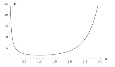 Figure 1
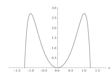 Figure 2
| 1 | 1 | 1 | 1 | 1 | |
|---|---|---|---|---|---|
| 1 | 0.555209 | 2.10126 | 1.18912 | 1.70538 | |
| 10 | 0.057703 | 173.590 | 1.22444 | 17.2831 | 10 |
| 100 | 0.005773 | 17320.9 | 1.22474 | 172.852 | 100 |
| 1 | |||
| 10 | 10 | 10 | |
| 100 | 100 | 100 |
| 0.01 | 2.33420 | 0.06531 | |
| 0.1 | 1.64821 | 0.23599 | |
| 1 | 1.25165 | 1.74866 | |
| 10 | 1.22505 | 17.2874 | 10 |
| 100 | 1.22475 | 172.853 | 100 |
Peer Reviews
No public reviews on file for this paper yet. If you reviewed it on a platform where reviews are public (OpenReview, ICLR, NeurIPS, ICML), you can paste yours below so the community can read it here.
Videos
No videos yet. Explain this paper in a talk, walkthrough, or lecture? Add one.
Analysis of big bounce in Einstein–Cartan cosmology
Jordan L. Cubero
Nikodem J. Popławski
Department of Mathematics and Physics, University of New Haven, 300 Boston Post Road, West Haven, CT 06516, USA
Abstract
We analyze the dynamics of a homogeneous and isotropic universe in the Einstein–Cartan theory of gravity. The spin of fermions produces spacetime torsion that prevents gravitational singularities and replaces the big bang with a nonsingular big bounce. We show that a closed universe exists only when a particular function of its scale factor and temperature is higher than some threshold value, whereas an open and a flat universes do not have such a restriction. We also show that a bounce of the scale factor is double: as the temperature increases and then decreases, the scale factor decreases, increases, decreases, and then increases.
Introduction. The Einstein–Cartan (EC) theory of gravity provides the simplest mechanism generating a nonsingular big bounce, without unknown parameters or hypothetical fields avert . EC is the simplest and most natural theory of gravity with torsion, in which the Lagrangian density for the gravitational field is proportional to the Ricci scalar, as in general relativity KS ; EC . The consistency of the conservation law for the total (orbital plus spin) angular momentum of fermions in curved spacetime with the Dirac equation allowing the spin-orbit interaction requires that the antisymmetric part of the affine connection, the torsion tensor Schr , is not constrained to zero req . Instead, torsion is determined by the field equations obtained from the stationarity of the action under variations of the torsion tensor. In EC, the spin of fermions is the source of torsion.
The multipole expansion Pap of the conservation law for the spin tensor in EC gives a spin tensor which describes fermionic matter as a spin fluid (ideal fluid with spin) NSH . Once the torsion is integrated out, EC reduces to general relativity with an effective spin fluid as a matter source EC . The effective energy density and pressure of a spin fluid are given by and , where and are the thermodynamic energy density and pressure, is the number density of fermions, and with HHK ; spin . The negative corrections from the spin-torsion coupling generate gravitational repulsion which prevents the formation of gravitational singularities and replaces the big bang with a nonsingular bounce, at which the universe transitions from contraction to expansion. These corrections lead to a violation of the strong energy condition by the spin fluid when drops below 0, thus evading the singularity theorems HHK . Accordingly, this violation could be thought of as the cause of the bounce.
The dynamics of the universe filled with a spin fluid in EC has been studied in spin . The expansion of the closed universe with torsion and quantum particle production shortly after a bounce is almost exponential for a finite period of time, explaining inflation ApJ . Depending on the particle production rate, the universe may undergo several bounces until it produces enough matter to reach a size where the cosmological constant starts cosmic acceleration. This expansion also predicts the cosmic microwave background radiation parameters that are consistent with the Planck 2015 observations Planck2015 , as was shown in SD .
The spin-fluid description of matter is the particle approximation of the multipole expansion of the integrated conservation laws in EC. The particle approximation for Dirac fields, however, is not self-consistent nons . The spin-fluid description also violates the cosmological principle viol . On the other hand, the Dirac form of the spin tensor for fermionic matter, which follows directly from the Dirac Lagrangian using the Sciama-Kibble variation with respect to the torsion tensor KS ; spinor , is consistent with the cosmological principle consist . The minimal coupling between the torsion tensor and Dirac fermions also averts the big-bang singularity Bounce ; also . Other forms of the torsion tensor in cosmology are investigated in other .
The spin-torsion coupling modifies the Dirac equation, adding a term that is cubic in spinor fields HD . As a result, fermions must be spatially extended nons , which could eliminate infinities arising in Feynman diagrams involving fermion loops. In the presence of torsion, the four-momentum operator components do not commute and thus the integration in the momentum space in Feynman diagrams must be replaced with the summation over the discrete momentum eigenvalues. The resulting sums are finite: torsion naturally regularizes ultraviolet-divergent integrals in quantum electrodynamics toreg . Torsion may also explain the matter-antimatter asymmetry anti and the cosmological constant cosmo .
The analysis in Bounce considered a closed, homogeneous, and isotropic universe in EC. However, the calculations of the maximum temperature and the minimum scale factor at a bounce neglected the factor in the Friedmann equations (which is justified during and after inflation but not at a bounce before inflation), de facto considering a flat universe. In addition, the time-dependence of the scale factor appeared to have a cusp-like behavior at the bounce. In this article, we refine those calculations by taking into account and analyzing the turning points of the universe for all three cases: (closed universe), (flat universe), and (open universe). We discover that a closed universe exists only when some function of the scale factor and temperature is higher than a particular threshold, whereas an open and flat universes are not restricted by this condition. Accordingly, a closed universe forms in a region of space within a trapped null surface when this threshold is reached. Such a region could be the interior of a black hole BH . Torsion therefore may explain the origin of our universe ApJ .
Dynamics of scale factor and temperature. If we assume that the universe is homogeneous and isotropic, then it is described by the Friedmann-Lemaître-Robertson-Walker metric, which is given in the isotropic spherical coordinates by
[TABLE]
where is the scalar factor as a function of the cosmic time LL2 . The Einstein field equations for this metric become the Friedmann equations:
[TABLE]
and
[TABLE]
where a dot denotes the derivative with respect to . The effective energy density and pressure for a Dirac field are given by spinor ; Bounce .
[TABLE]
where
[TABLE]
Multiplying the first Friedmann equation by and differentiating over time, and subtracting from it the second Friedmann equation multiplied by gives an equation that has the form of the first law of thermodynamics for an adiabatic universe:
[TABLE]
which gives
[TABLE]
The matter in the early universe is ultrarelativistic. If we assume kinetic equilibrium, then we can use , , and , where is the temperature of the universe, , and Ric . The quantities and are the numbers of spin states for all elementary bosons and fermions, respectively. For standard-model particles, and . In the presence of spin and torsion, the first Friedmann equation is therefore Bounce
[TABLE]
The first law of thermodynamics (7) gives
[TABLE]
or
[TABLE]
where
[TABLE]
is the critical temperature. Equation (10) determines the scale factor as a function of temperature and can be integrated to
[TABLE]
where is an integration constant. This constant is positive because the scale factor and temperature are positive.
We define nondimensional quantities:
[TABLE]
where
[TABLE]
Henceforth, we will use a dot to denote the derivative with respect to the new time coordinate . Equation (8) can be written, using these quantities, as
[TABLE]
Equation (12) can be written as
[TABLE]
where is a positive constant, related to by
[TABLE]
Substitution of in Eq. (18) into Eq. (17) gives
[TABLE]
The function , given by Eq. (18), has a minimum at (), and its value is
[TABLE]
This minimum determines the minimum value of the scale factor:
[TABLE]
Consequently, the scale factor cannot reach zero. The universe with spin and torsion is nonsingular for all three cases of and for all values of . Figure 1 shows the function (18) for .
Turning points in a closed universe. Let us consider a closed relativistic universe, for which . The turning points for this universe are determined by the condition , for which Eq. (20) gives
[TABLE]
Figure 2 shows a curve representing the function on the left-hand side of Eq. (23). This function has a maximum at and its value is . Equation (23) has solutions whose number depends on the value of . We only consider the solutions with a physical condition . This equation has two turning points (points of intersection of the curve in Fig. 2 with a horizontal line ) if the line lies below the maximum of the curve, that is, if
[TABLE]
The segment of the curve above this line corresponds to in Eq. (20). Consequently, the universe would oscillate between the two values of at the points of intersection: (big bounce) and (big crunch). If , Eq. (20) has one turning point at . The universe would be stationary at a constant temperature. If , Eq. (20) has no turning points and the universe would not exist.
Table 1 shows the values of and for a closed universe for different values of . As tends to infinity, the value of tends to which results from Eq. (23) reducing for small values of to . In the same limit, the value of tends to which is an -intercept of the curve in Fig. 2 and sets the maximum temperature in the universe.
Table 1 also shows the values of corresponding to and , given by Eq. (18), and the value of , given by Eq. (21), for different values of . The value of is evidently greater than the corresponding value of . As tends to infinity, tends to , whereas tends to . In the same limit, the ratio tends to , to , and to .
Turning points in a flat universe. Let us consider a flat relativistic universe, for which . The turning points for this universe are determined by the condition , for which Eq. (20) gives
[TABLE]
This equation has two physical solutions (points of intersection of the curve in Fig. 2 with the -axis). They are given by and . The segment of the curve above the -axis corresponds to in Eq. (20). Consequently, the temperature of the universe lies between and . As tends to 0, tends to infinity and , which is positive, asymptotically tends to zero. Therefore, a flat universe has only one turning point at . This value coincides with that of for a closed universe in the limit . The corresponding value of is which is evidently greater than given by (21).
Table 2 shows the values of and for a flat universe for different values of . The values of and are -intercepts of the curve in Fig. 2. Table 2 also shows the values of corresponding to and , given by Eq. (18), and the value of , given by Eq. (21), for different values of .
Turning points in an open universe. Let us now consider an open relativistic universe, for which . The turning points for this universe are determined by the condition , for which Eq. (20) gives
[TABLE]
This equation has one physical solution (point of intersection of the curve in Fig. 2 with a horizontal line ). It is given by . Therefore, an open universe has only one turning point at . The segment of the curve above this line corresponds to in Eq. (20). Evidently, . As tends to 0, tends to infinity and , which is positive, asymptotically tends to 1.
Table 3 shows the values of and for different values of . As tends to infinity, the value of tends to , as for a closed universe, which is an -intercept of the curve in Fig. 2 and equal to for a flat universe. Table 3 also shows the values of corresponding to and , given by Eq. (18), and the value of , given by Eq. (21), for different values of . The value of is evidently greater than the corresponding value of . As tends to infinity, tends to , as for a closed universe.
Time dynamics near a bounce. Differentiation of Eq. (18) with respect to gives
[TABLE]
Substitution of this into Eq. (17) gives
[TABLE]
which determines the function , and with Eq. (18), the function . Equation (27) shows that if or . As tends to 1, we have
[TABLE]
Accordingly, as , : the function has a vertical inflection point.
Equation (17) for , at which is a minimum of the function , gives
[TABLE]
This equation has solutions for all allowed values of . If and the condition (24) is satisfied, or if or , then at . It can be shown, by differentiation of Eq. (27) with respect to , that the function has a local minimum at and a local maximum when ().
Accordingly, the following scenario occurs. As the universe contracts, decreases and increases. When reaches 1, reaches a local minimum (a bounce) and exhibits vertical inflection. Then, continues to increase, but also increases. When reaches , reaches a local maximum. Then, begins to decrease, but also decreases. When reaches 1, reaches a local minimum (another bounce) and exhibits vertical inflection. Then, continues to decrease and increases. Consequently, at a bounce, the universe has a single bounce of the temperature and a double bounce of the scale factor with a little crunch between the two bounces. If the value of remains constant, then the double bounce of the scale factor is symmetric. Otherwise, it is asymmetric.
Conclusions. We analyzed the dynamics of a homogeneous and isotropic universe in the Einstein–Cartan theory of gravity. The coupling between the spin of fermions and torsion prevents a cosmological singularity, replacing the big bang with a nonsingular big bounce, at which the universe transitions from contraction to a short period of expansion, followed by a short period of contraction, followed by expansion (double bounce of the scale factor). We eliminated the problem of a cusp that was reported earlier in Bounce . We showed that a closed universe may exist only when some function of the scale factor and temperature is higher than a particular threshold. Equation (18) and inequality (24) give
[TABLE]
On the other hand, a flat universe and an open universe can exist for all positive values of the integration constant .
The formation of a closed universe corresponds to the moment when the quantity begins to satisfy the inequality (24) in a region of space within a trapped null surface. During inflation, this quantity increases ApJ , possibly because of quantum particle-pair production in strong gravitational fields. For large values of , can become small when becomes large, as shown in Table 1. In this range, Eq. (18) reduces to the torsionless limit:
[TABLE]
and the universe transitions from the torsion-dominated era to the radiation-dominated era. The quantity begins to represent the product of the scale factor and temperature. Eventually, the universe reaches the matter-dominated era and then dark-energy-dominated era. Inflation must increase the value of to a threshold sufficient for the universe to reach the size at which dark energy can start the observed current acceleration ApJ . Otherwise, the universe would undergo several temperature bounces, accompanied by double scale factor bounces, before reaching this threshold SD .
Acknowledgment. This work was funded by the University Research Scholar program at the University of New Haven.
The reference list from the paper itself. Each links out to its DOI / PubMed record.
- 1(1) W. Kopczyński, Phys. Lett. A 39 , 219 (1972); Phys. Lett. A 43 , 63 (1973); A. Trautman, Nature (Phys. Sci.) 242 , 7 (1973).
- 2(2) T. W. B. Kibble, J. Math. Phys. 2 , 212 (1961); D. W. Sciama, in Recent Developments in General Relativity , p. 415 (Pergamon, 1962); Rev. Mod. Phys. 36 , 463 (1964); Rev. Mod. Phys. 36 , 1103 (1964).
- 3(3) E. A. Lord, Tensors, Relativity and Cosmology (Mc Graw-Hill, 1976); F. W. Hehl, P. von der Heyde, G. D. Kerlick, and J. M. Nester, Rev. Mod. Phys. 48 , 393 (1976); V. de Sabbata and M. Gasperini, Introduction to Gravitation (World Scientific, 1985); K. Nomura, T. Shirafuji, and K. Hayashi, Prog. Theor. Phys. 86 , 1239 (1991); V. de Sabbata and C. Sivaram, Spin and Torsion in Gravitation (World Scientific, 1994); N. J. Popławski, ar Xiv:0911.0334.
- 4(4) E. Schrödinger, Space-time Structure (Cambridge University Press, 1954).
- 5(5) F. W. Hehl and J. D. Mc Crea, Found. Phys. 16 , 267 (1986); N. Popławski, ar Xiv:1304.0047.
- 6(6) A. Papapetrou, Proc. Roy. Soc. London A 209 , 248 (1951).
- 7(7) K. Nomura, T. Shirafuji, and K. Hayashi, Prog. Theor. Phys. 86 , 1239 (1991).
- 8(8) F. W. Hehl, P. von der Heyde, and G. D. Kerlick, Phys. Rev. D 10 , 1066 (1974).