The low-frequency break observed in the slow solar wind magnetic spectra
R. Bruno, D. Telloni, L. Sorriso-Valvo, R. Marino, R. De Marco, R., DAmicis

TL;DR
This study reveals that the low-frequency 1/f magnetic spectral break, previously observed only in fast solar wind streams, also exists in slow streams when sufficiently long intervals are analyzed, challenging prior assumptions.
Contribution
The paper demonstrates, for the first time, that the 1/f magnetic spectral scaling is present in slow solar wind when long-lasting intervals are examined, extending previous findings.
Findings
The 1/f magnetic spectral scaling exists in slow wind for long intervals.
Velocity spectrum maintains Kolmogorov scaling regardless of interval length.
Magnetic amplitude saturation may explain the 1/f scaling in slow wind.
Abstract
Fluctuations of solar wind magnetic field and plasma parameters exhibit a typical turbulence power spectrum with a spectral index ranging between and . In particular, at AU, the magnetic field spectrum, observed within fast corotating streams, also shows a clear steepening for frequencies higher than the typical proton scales, of the order of Hz, and a flattening towards at frequencies lower than Hz. However, the current literature reports observations of the low-frequency break only for fast streams. Slow streams, as observed to date, have not shown a clear break, and this has commonly been attributed to slow wind intervals not being long enough. Actually, because of the longer transit time from the Sun, slow wind turbulence would be older and the frequency break would be shifted to lower frequencies with respect to…
Click any figure to enlarge with its caption.
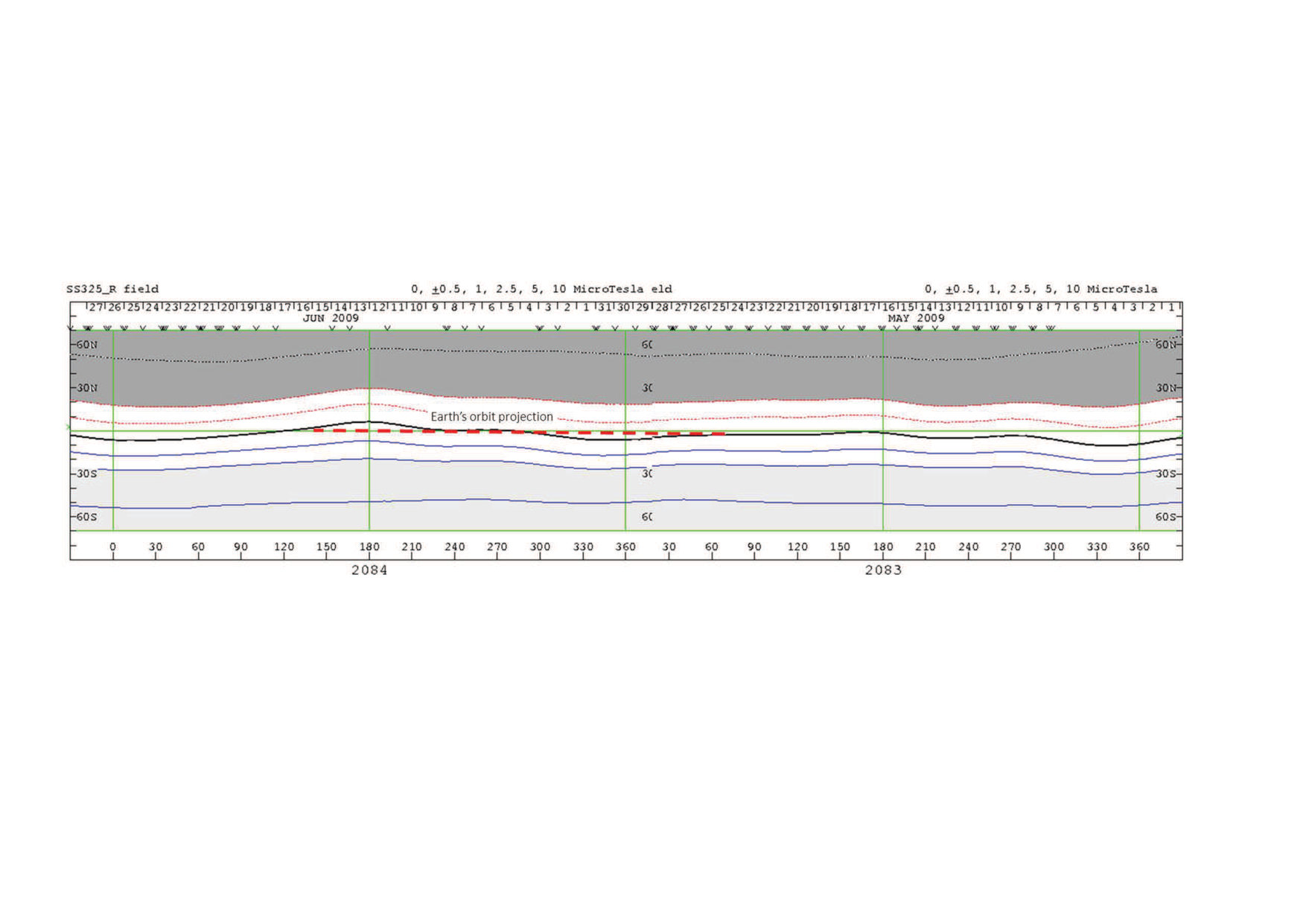 Figure 1
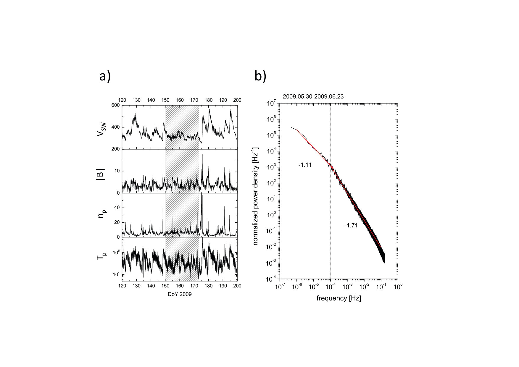 Figure 2
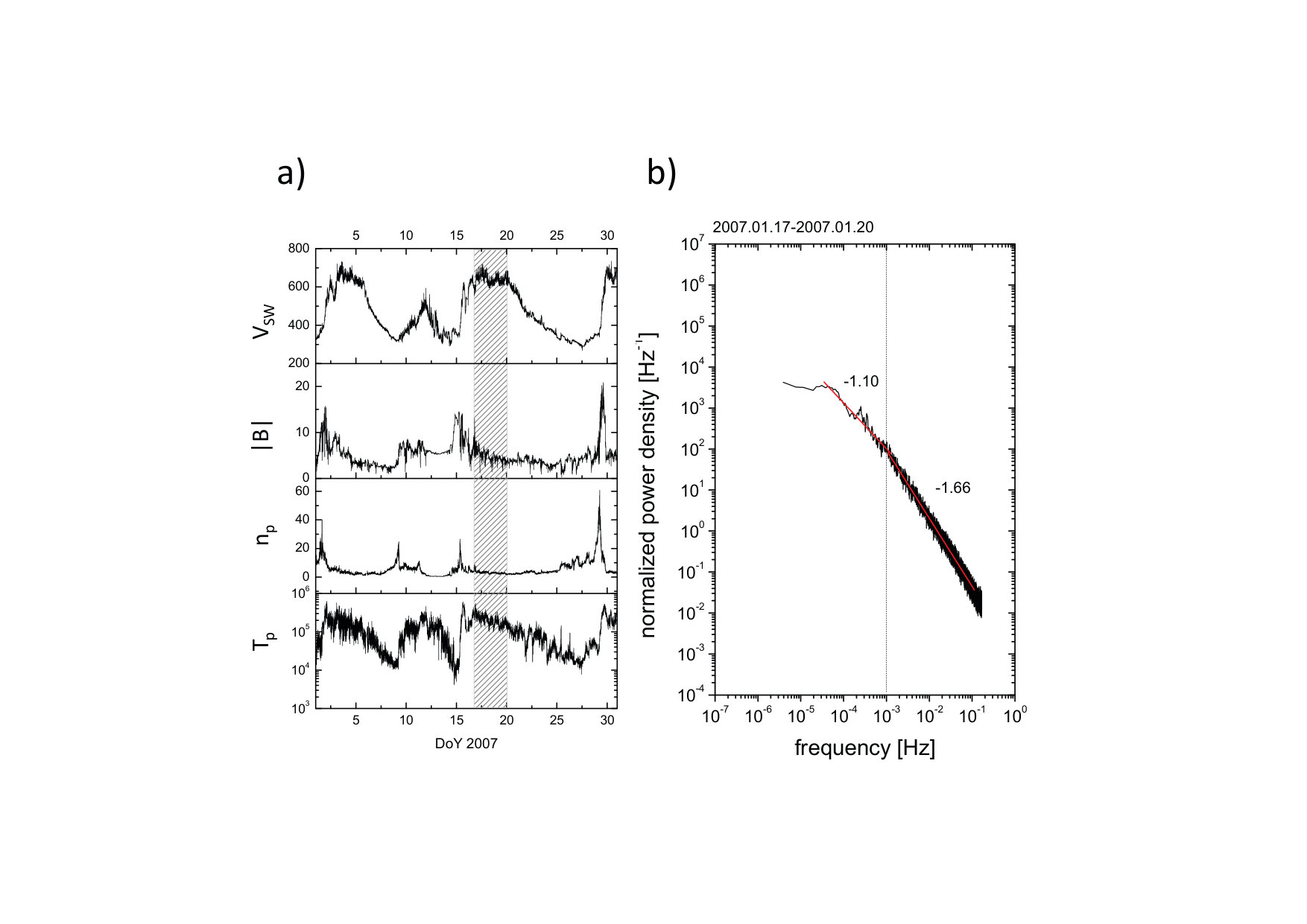 Figure 3
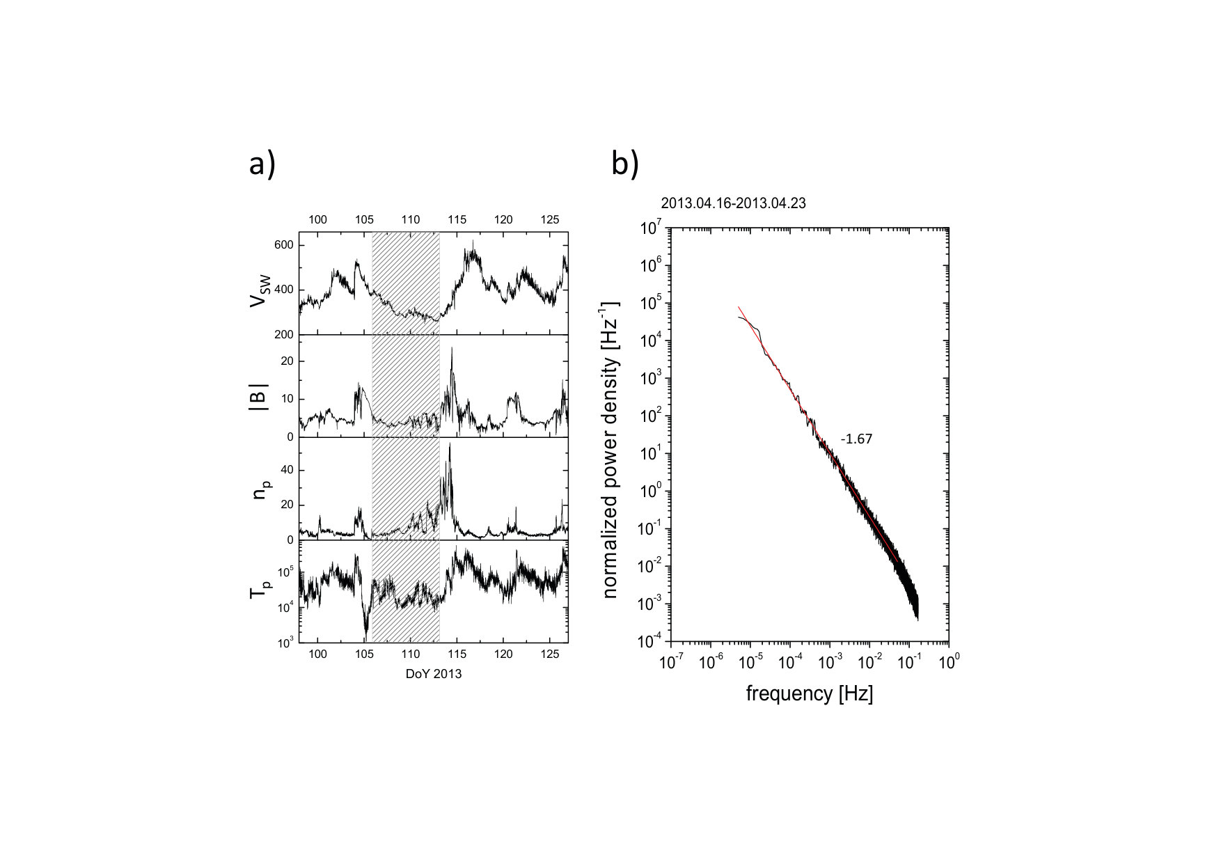 Figure 4
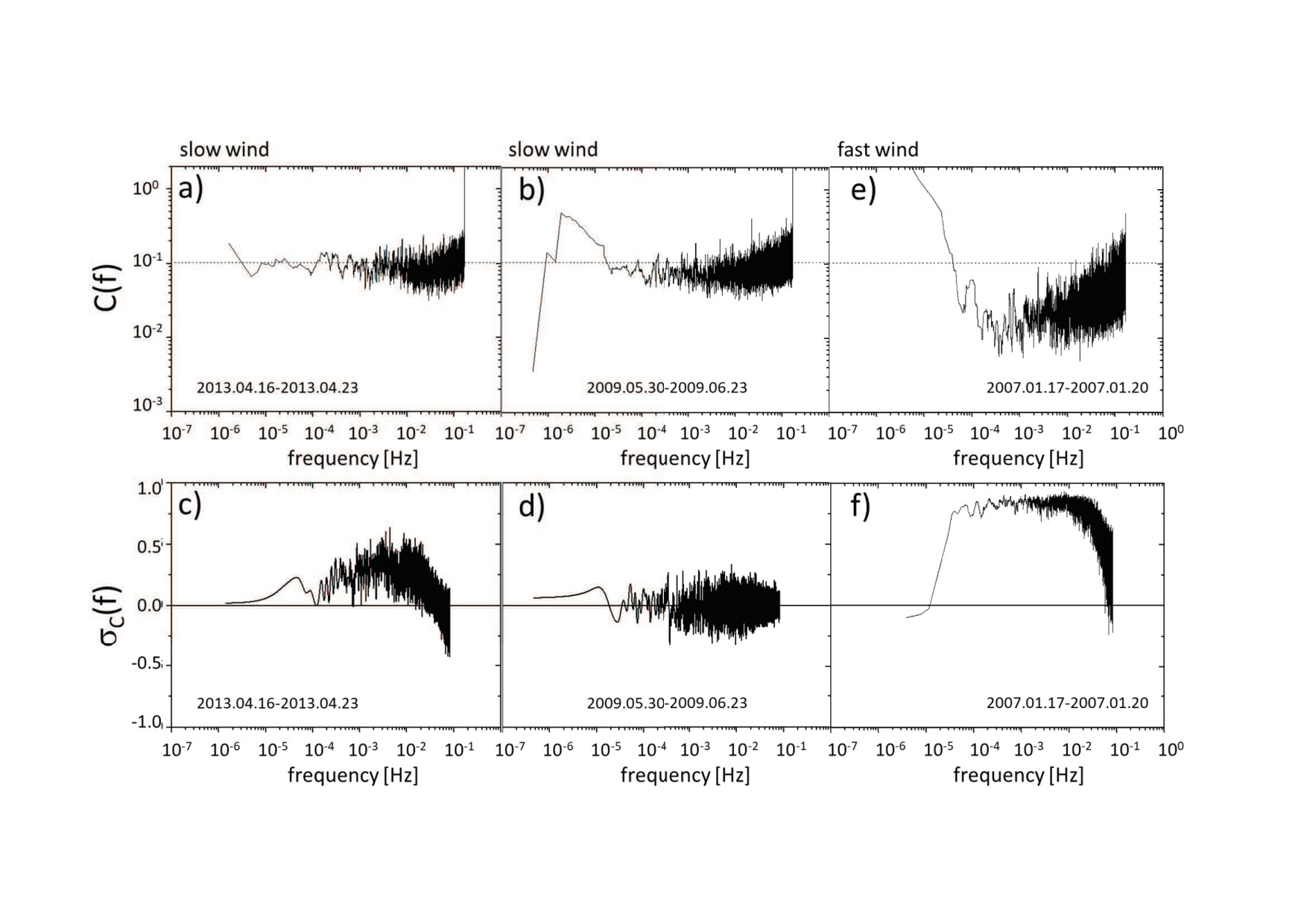 Figure 5
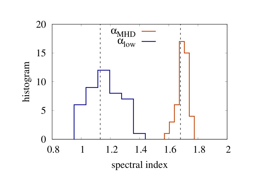 Figure 6
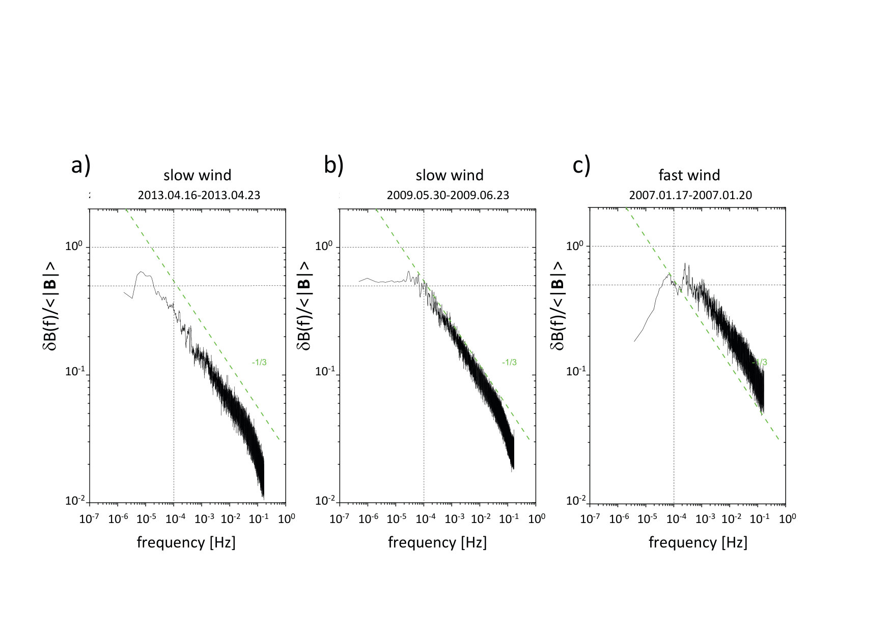 Figure 7
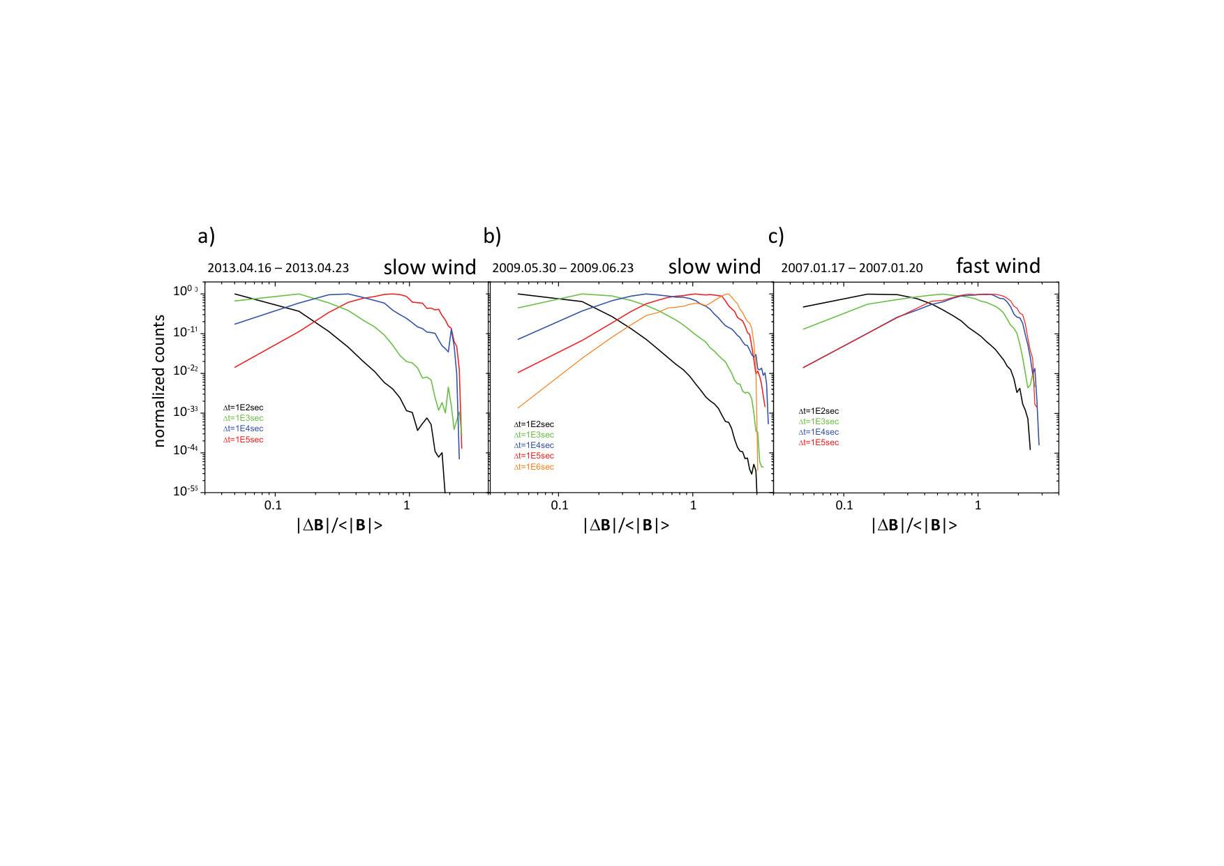 Figure 8
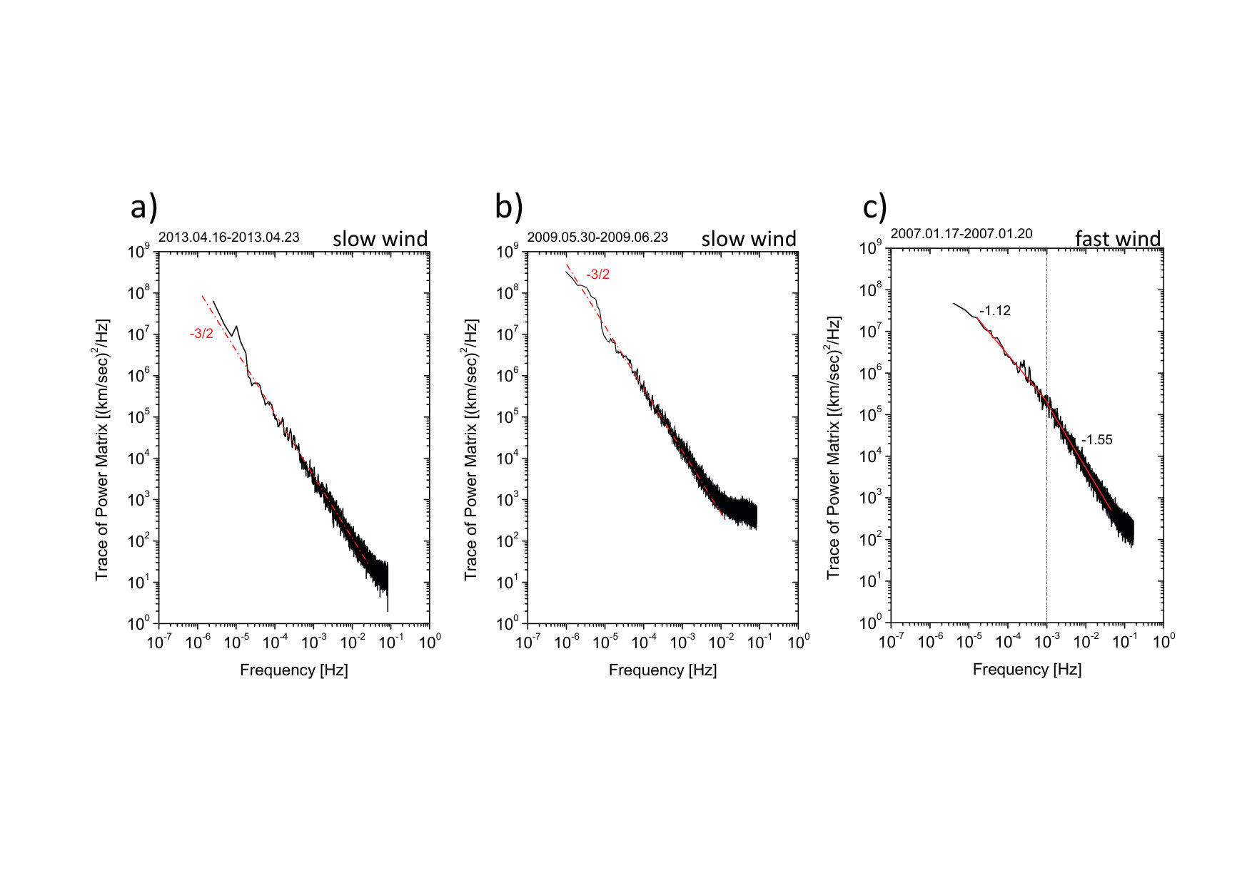 Figure 9
Peer Reviews
No public reviews on file for this paper yet. If you reviewed it on a platform where reviews are public (OpenReview, ICLR, NeurIPS, ICML), you can paste yours below so the community can read it here.
Videos
No videos yet. Explain this paper in a talk, walkthrough, or lecture? Add one.
11institutetext: National Institute for Astrophysics, Institute for Space Astrophysics and Planetology, Via del Fosso del Cavaliere 100, 00133 Roma, Italy 22institutetext: National Institute for Astrophysics, Astrophysical Observatory of Torino, Via Osservatorio 20, 10025 Pino Torinese, Italy 33institutetext: Departamento de Física, Escuela Politécnica Nacional, Quito, Ecuador 44institutetext: Nanotec/Consiglio Nazionale delle Ricerche, ponte P. Bucci, cubo 31C, I-87036 Rende (CS), Italy 55institutetext: Laboratoire de Mécanique des Fluides et d’Acoustique, CNRS, École Centrale de Lyon, Université Claude Bernard Lyon 1, INSA de Lyon, F-69134 Écully, France
The low-frequency break observed in the slow solar wind magnetic spectra
R. Bruno 11
D. Telloni 22
L. Sorriso-Valvo 3344
R. Marino 55
R. De Marco 11
R. D’Amicis 11
(Received ; accepted )
Fluctuations of solar wind magnetic field and plasma parameters exhibit a typical turbulence power spectrum with a spectral index ranging between and . In particular, at AU, the magnetic field spectrum, observed within fast corotating streams, also shows a clear steepening for frequencies higher than the typical proton scales, of the order of Hz, and a flattening towards at frequencies lower than Hz. However, the current literature reports observations of the low-frequency break only for fast streams. Slow streams, as observed to date, have not shown a clear break, and this has commonly been attributed to slow wind intervals not being long enough. Actually, because of the longer transit time from the Sun, slow wind turbulence would be older and the frequency break would be shifted to lower frequencies with respect to fast wind. Based on this hypothesis, we performed a careful search for long-lasting slow wind intervals throughout years of Wind satellite measurements. Our search, based on stringent requirements not only on wind speed but also on the level of magnetic compressibility and Alfvénicity of the turbulent fluctuations, yielded slow wind streams lasting longer than days. This result allowed us to extend our study to frequencies sufficiently low and, for the first time in the literature, we are able to show that the magnetic spectral scaling is also present in the slow solar wind, provided the interval is long enough. However, this is not the case for the slow wind velocity spectrum, which keeps the typical Kolmogorov scaling throughout the analysed frequency range. After ruling out the possible role of compressibility and Alfvénicity for the scaling, a possible explanation in terms of magnetic amplitude saturation, as recently proposed in the literature, is suggested.
Key Words.:
(Sun:) solar wind – turbulence – waves – heliosphere – magnetic fields – plasmas
1 Introduction
The properties of heliospheric magnetic field and particle velocity fluctuations have been studied for decades with the major aim of understanding the mechanisms that govern the dynamics of the collisionless solar system plasmas (Bruno & Carbone,, 2013). The measurements provided by several spacecraft have allowed us to determine that the solar wind expansion is highly turbulent, as suggested by the ubiquitous observation of Kolmogorov-like magnetic field and velocity power spectra (Kolmogorov,, 1941; Frisch,, 1995; Tu & Marsch,, 1995; Bruno & Carbone,, 2013; Tsurutani et al., 2018).
At the low-frequency end of the spectra, the fast and Alfvénic solar wind often displays a robust scaling range ( being the frequency), which has been interpreted as injection range for the turbulent energy cascade. This was observed both in the ecliptic and in the polar solar wind (Bruno et al., 2009; Horbury et al., 1996; Matthaeus et al., 2007), for both magnetic field and velocity, but the reason for the formation of such scaling is still an open question.
Indeed, a range over which the low-frequency spectrum of physical quantities follows power-law scalings close to is observed in a variety of turbulent systems, for instance in geophysical fluids (Fraedrich & Blender,, 2003; Costa et al.,, 2014), in flow simulations in laboratory (Herault et al.,, 2015; Pereira et al.,, 2019), and in numerical simulations of hydrodynamic (HD) and magnetohydrodynamic (MHD) flows (Dmitruk & Matthaeus,, 2007).
Moreover, evidence of long-period fluctuations associated with the low-frequency spectrum have been provided by Dmitruk et al., (2011) in HD and MHD systems allowing condensation of invariants (or quasi-invariants) at the lowest wave-number mode. This is the case for three-dimensional MHD plasmas (with or without a background magnetic field) and for rotating HD flows where inverse cascades of helicity or energy can indeed develop and have been associated with the onset of a low-frequency spectrum in direct numerical simulations (Dmitruk et al.,, 2011).
However, limiting ourselves to interplanetary space plasmas, it is worth mentioning some past and current views on the nature of the scaling range. For example, Nakagawa & Levine (1974) pointed out the possible link between the scaling in the interplanetary magnetic field and the structured surface of the Sun, based on early observations of a clear ( being the wavenumber) spectral region in the solar photospheric magnetograms. Instead, Matthaeus & Goldstein (1986) proposed that this kind of scaling could be the result of the early (i.e. within the Alfvénic radius) superposition of uncorrelated samples of turbulence, whose correlation lengths are lognormally distributed, each originating at a different regions of the solar surface. As shown by Montroll & Shlesinger (1982), a similar superposition of turbulence samples, in certain circumstances, can produce a scaling. A different interpretation was given in terms of outward travelling low-frequency waves propagating from the coronal base, whose superposition could generate the magnetic field and density spectrum. In this framework, the range was not present in purely hydrodynamic simulations, suggesting the central role of the magnetic field in its production (Dmitruk et al.,, 2002, 2004). Consolini et al. (2015), using numerical simulations based on a shell model, obtained the formation of such a spectral domain in both fluid and MHD cases. These authors explained the emergence of such a domain in terms of a competition between direct and inverse energy cascading at the sub-inertial scales. Recent studies point to the possibility that the emergence of coherent structures and/or the condensation of energy on large scales could be the origin of the low-frequency spectrum in fluid and plasma turbulence. In particular, it has been shown in liquid metal experiments (at high Reynolds number) that three-dimensional shear flows and quasi-two-dimensional flows both exhibit a low-frequency spectrum, due to an increase in power in the gravest modes, caused respectively by the instability of the shear layer (Pereira et al.,, 2019) and the onset of a large-scale circulation (Herault et al.,, 2015).
Velli et al. (1989) and then Verdini et al. (2012) and Tenerani & Velli (2017) suggested that outward propagating modes could be reflected by large-scale solar wind gradients in the extended solar corona, and their non-linear interaction would result in a turbulent cascade with spectral scaling , already visible within the sub-Alfvénic solar wind . The latest interpretation is due to Matteini et al., (2018) who suggested that the spectrum could be due to the saturation of the magnetic field Alfvénic fluctuations to the limiting value represented by the magnetic magnitude.
The analysis of the magnetic field spectral properties in the expanding solar wind showed a clear radial evolution of the frequency of the break between the region and the typical Kolmogorov fully developed turbulence. In particular, the break frequency decreases with the heliocentric distance roughly as a power law for fast ecliptic wind (Bruno & Carbone,, 2013) ( for fast polar wind (Horbury et al., 1996)). A similar evolution, but with a slower decrease (), was also observed for the spectral break between the Kolmogorov range and the high-frequency kinetic range (Bruno & Trenchi,, 2014). These observations suggested that the turbulence could develop as the solar wind travels away from the Sun, involving progressively larger scales into the turbulent cascade. This radial evolution increases the extension of the inertial range of solar wind turbulence, and consequently of the Reynolds number (Matthaeus et al.,, 2005; Telloni et al., 2015).
Contrary to the fast solar wind, the analysis of the spectra of slow wind (i.e. solar wind streams with bulk speed km s*-1*) provided evidence of Kolmogorov scaling all the way down to the low-frequency range (Bruno & Carbone,, 2013). Based on our present interpretation of the observed phenomenology and on the basis of available models, this is not surprising since the slow wind turbulence has more time to develop during its slower expansion, thus allowing the possible low-frequency spectral break to drift towards lower frequencies than in the fast wind. If this is the case, then we can expect to be able to observe the low-frequency break only in particularly long wind samples, where the low-frequency spectral properties can be properly captured.
In this paper we provide the first evidence of the existence of the low-frequency break and of a spectral scaling in a selection of slow wind samples. We then discuss the possible origin of this scaling in the framework of the interpretations listed above.
2 Data analysis
In order to study the low-frequency spectral properties of the slow solar wind, we performed a systematic search for slow wind intervals using years’ worth of solar wind observations recorded by the Wind spacecraft between and . The following plasma and magnetic field data sets were used throughout the analysis: the Wind 3DP, PESA-LOW (Lin et al.,, 1995) onboard computed ion moments (proton and particles) sec (spin) resolution, and the Wind Magnetic Field Investigation (MFI) experiment (Lepping et al.,, 1995) sec averages, respectively. Considering the slight changes in the plasma sampling time during the mission, these two data sets were interpolated and re-sampled with a six-second cadence in order to allow for a synchronized study.
Our selection of slow wind intervals was based on the evaluation of the following parameters: wind speed, time duration, magnetic intensity variability and Alfvénicity. The solar wind speed had to be consistently small ( km s*-1*) for an interval of at least 7 days in order to extend our study to sufficiently low frequencies. The time interval should not contain strong transient events or shocks which would alter the magnetic field compressibility and the average value of the normalized standard deviation of the field intensity , estimated at hourly scale, should not exceed the value of . Finally, the Alfvénicity of the fluctuations, estimated at hourly scales by the normalized cross-helicity (defined as , where and are the velocity and magnetic field vector fluctuations and and are the kinetic and magnetic energy, respectively) should be less than . This last requirement allows us to exclude from our data set the Alfvénic slow wind, recently studied by D’Amicis & Bruno (2015) and D’Amicis et al. (2019), which is more similar to the fast Alfvénic wind than to the slow wind analysed in this work.
These selection criteria allowed us to identify 48 time intervals, which we found to be randomly distributed within the 12 years under study. The resulting data set was primarily used to evaluate solar wind velocity spectra and the Alfvénicity of the fluctuations within each of the selected time intervals. Additionally, given the better resolution and completeness of the magnetic field measurements, magnetic spectra, and magnetic compressibility were evaluated using the three-second cadence data, providing a more robust estimate.
Among the 48 selected cases, we show one example relative to one of the longest and most representative streams, recorded from day to of . During this -day interval, the Earth’s heliographic latitude changed from to . Because of the specific configuration of the heliomagnetic equator during the observation time, the Earth was steadily close to the ecliptic current sheath during the whole time interval. This particular configuration can be observed in Fig. 1, showing the source surface synoptic maps of Carrington Rotation and from the Wilcox Solar Observatory, as inferred at solar radii.
Some relevant solar wind parameters relative to this time interval are shown in the shaded area of panel a of Fig. 2, which spans from day to of year . Such extremely long time intervals, characterized by an almost steady slow wind speed, are uncommon and this explains the reason for the limited number of intervals that satisfy our search criteria within 12 years of data. The speed profile of the selected interval (shaded area) does not show large variability, with an average value of km s*-1*, while the other parameters show the typical variability of slow wind. Panel b of Fig. 2 shows the total power density spectrum, i.e. the trace of the spectral matrix, normalized to the square value of the mean magnetic field intensity. This figure represents the first evidence of the existence of the low-frequency break within the slow solar wind. The vertical dashed line separates the high-frequency range, characterized by about three decades of typical quasi-Kolmogorov scaling with exponent close to -5/3, and the low-frequency range, showing a power-law scaling with exponent close to -1 and extending for more than two decades. To the best of our knowledge, this is a new observation that was never reported in the literature. In the example shown here, the low-frequency spectral break is located around Hz, about one order of magnitude lower than the typical values observed in the fast solar wind, closer to Hz (Bruno & Carbone,, 2013). This implies that particularly extended intervals are necessary in order to observe the scaling in the slow solar wind.
It is interesting to compare this value with the break location predicted by the radial dependence valid for the fast wind in the ecliptic (Bruno & Carbone,, 2013). To do this, we analyse a typical fast wind interval highlighted by the dashed area in panel a of Fig. 3. This is a typical corotating, high-velocity stream characterized by an average speed of km s*-1*. Panel b of Fig. 3 shows the relative trace of the power density spectral matrix of the magnetic field fluctuations. This spectrum, as expected, shows a frequency break around Hz, a typical value for fast wind (Bruno & Carbone,, 2013). A lower expansion speed implies a longer transport time which, in turn, implies older turbulence. Given the linear relationship between transport time, velocity, and radial distance we can estimate the frequency break location at AU for our slow wind from the frequency break of the fast wind and the radial dependence reported by Bruno & Carbone, (2013):
[TABLE]
The estimate from Eq. (1) provides a value higher than Hz shown in Fig. 2. Although this value should be taken as a rough estimate, we verified that this discrepancy is not an isolated case, but generally applies to the break location observed for the slow wind at AU, although within a certain variability. Thus, the location of the slow wind break does not seem to be regulated by the age of turbulence as estimated from Eq. (1), and the reason for this discrepancy might have a different origin.
However, a long enough time interval of slow wind seems to be a necessary but not sufficient condition to have a clear low frequency break. In panel a of Fig. 4, we show another example of slow wind interval where the low-frequency break is clearly absent, in spite of the remarkably long duration of this sample. The example shown here refers to a slow wind time interval lasting seven days and moving with an average flow speed of km s*-1*. The magnetic field power spectrum is shown in panel b of the same figure, and is characterized by a typical Kolmogorov scaling throughout the whole frequency range, for about four decades, with no observable low-frequency break up to scales of about one day. In this case, Eq. (1) would predict a frequency break at Hz.
A remarkable difference between the two examples of slow wind shown in Figs. 2 and 4 is found in the normalized spectral power level. Indeed, the spectrum without a low-frequency break (Fig. 4) has much less power than the one with the break (Fig. 2). This observation is particularly relevant and is discussed in the following paragraphs.
We compared other turbulence aspects of these two time intervals. In particular, we looked at magnetic compressibility and Alfvénicity. To evaluate the compressibility we estimated the ratio between the power associated to magnetic field intensity fluctuations and the total magnetic energy, namely the trace of the spectral matrix, (Bavassano et al.,, 1982). On the other hand, the degree of Alfvénicity was evaluated computing, as is customary, the normalized cross-helicity in terms of Elssser variables, where and are the total power associated with outward and inward Alfvénic fluctuations, respectively (Bruno & Carbone,, 2013). In Fig. 5 we show plots of and versus frequency, for the two time intervals shown in Figs. 4 and 2. These two parameters do not display substantial differences for the two time intervals: the level of magnetic compressibility is low and very similar (panels a and b), and the Alfvénicity (panels c and d) shows only a rather modest difference, being slightly larger for the second interval not characterized by the frequency break. Such a difference, however, does not seem to explain the absence of the spectral break for the corresponding time interval, since enhanced Alfvénicity and low compressibility, as shown in panels e and f relative to the fast stream of Fig. 3, are always associated with the clear presence of a low-frequency break (Bruno & Carbone,, 2013).
The analysis of the magnetic spectral properties of the selected intervals robustly shows the presence of a Kolmogorov-like scaling in the inertial range, roughly located between Hz and Hz. The average spectral index is , the error being the standard deviation over the cases, and is in agreement with the literature (Bruno & Carbone,, 2013). Figure 6 shows the histogram of the exponents (in red), revealing the narrow dispersion associated with the magnetohydrodynamic inertial range spectral decay.
At lower frequencies, the survey provided the following possible behaviours: (i) the Kolmogorov inertial range extends to all observed frequencies (observed in 4 samples, or 8% of the cases; see the example in Fig. 4); (ii) there is evidence of a low-frequency spectral break, but no well-defined large-scale power law (6 samples, 13%); (iii) there is a well-defined power law for at least one frequency decade below the low-frequency break (38 samples, 79%; see the example in Fig. 2); and (iv) the spectrum shows a flat (white noise) region at the lower frequencies, after a low-frequency break—thus excluding the cases of group (i)—but irrespective of the presence or absence of power-law scaling—thus joining the cases of groups (ii) and (iii)—(12 samples, 25%).
When a power law is observed, the average spectral index is , and its distribution given in panel b of Fig. 6 shows a broader variability than for the inertial range. The predominant number of cases with a power law observed above (i.e. group (ii), including nearly of the samples) demonstrates that extended intervals of slow solar wind with low compressibility are predominantly characterized by a typical low-frequency spectral range.
3 Discussion
The reasons for different spectral behaviour observed in the slow wind intervals analysed for this work could be due to the different characteristics of the fluctuations forming the turbulence spectrum. To explore this possibility, for each of the slow wind streams we evaluated the level of compressibility and Alfvénicity of the turbulent fluctuations, but the results were similar to those shown in Figure 5, not showing any particular correlation between these parameters and the spectral form.
At this point, we checked whether a saturation effect of the fluctuations, similar to that suggested by Matteini et al., (2018) for the fast Alfvénic wind, could also play a role in the slow wind spectral break. Thus, in order to explore this possibility, differently from Matteini et al., (2018) who used first-order structure functions, we estimated the amplitude of each Fourier mode using the simple relation that binds together the power of a given fluctuation and the amplitude of the fluctuation , by means of the Fourier power spectral density , namely . These values were successively normalized to the corresponding local magnetic field average within each interval and are shown in Fig. 7. Panel a refers to the slow wind interval of Fig. 4, characterized by an extended Kolmogorov spectrum and no range; panel b refers to the slow wind interval of Fig. 2, which shows the scaling; and panel c refers to the fast wind interval of Fig. 3, which shows (as expected for the fast wind) an extended Kolmogorov spectrum and a clear scaling. In all panels, the green dashed line is an arbitrary reference level with the expected scaling for the amplitude of the Fourier modes. This line has been drawn to facilitate the comparison between the different levels of in the three panels.
Since these plots directly derive from their corresponding normalized power density spectra shown in Figs. 2, 3, and 4 we observe a flattening in the same frequency range where the power density spectra shows the scaling. In other words, the flattening indicates that the amplitude of the Fourier modes has reached a limit, i.e., below a certain frequency the fluctuations are saturated. This particular condition is reached at higher and higher frequencies depending on the relative amplitude of the fluctuations with respect to the local field. This is evident moving from panel a to panel c of Fig. 7.
As already recalled before, Matteini et al., (2018) suggested that the scaling observed in fast wind magnetic field might be the consequence of the large-scale saturation of the fluctuations. In this perspective, the amplitude of the fluctuations would be limited by the magnitude of the local magnetic field. The results shown here would expand this interpretation of the range to the slow solar wind.
In order to strengthen this interpretation with additional experimental evidence we show, in Fig. 8, the histograms of the normalized amplitude of the magnetic field fluctuations , where is the timescale and is the average value of the field intensity within the selected time interval. If the magnetic field intensity did not change with time, would have a limiting value of . Each curve in each panel has been normalized to its maximum value. The three panels a, b, and c correspond to the three different time intervals described in Fig. 4, Fig. 2, and Fig. 3, respectively. The different timescales are indicated by the colour-coding shown in each panel. Panel a corresponds to the slow wind interval without magnetic field spectral break, while panel b corresponds to the time interval which shows the break. The different histograms in panels a, b, and c refer to four different timescales, namely , and sec. In addition, given the remarkable length of the corresponding time interval, panel b also shows the histogram for the timescale sec. It is interesting to note that increasing the timescale moves the peak of the corresponding histogram to higher values of in each panel. However, only for panels b and c do the curves display their maximum value around and, in particular, only the histograms corresponding to the timescales falling within the spectral range in Fig. 2b (slow wind) and Fig. 3b (fast wind) tend to collapse on each other. This phenomenon is a clear indication that fluctuations become saturated starting at the timescale where the peak of the corresponding histogram is around . Obviously, this limiting value can be larger than depending on the compressive level of the fluctuations, being exactly only if the magnetic field vector fluctuates on the surface of a sphere of constant radius. To this regard, it is worth mentioning that Tsurutani et al. (2018), studying a low-compression high-speed stream, did find Alfvénic fluctuations whose amplitudes were equal to the entire magnetic field strength. However, we like to remark that for the slow wind cases analysed in this work, the saturation effect is not due to Alfvénic fluctuations but rather to different local orientations of the magnetic field reflecting the background field within adjacent static structures advected by the wind (Bruno et al., 2004). These results show that the phenomenon of saturation of magnetic field fluctuations is common to both fast and slow winds. In other words, it appears that it is not the nature of the fluctuations but their amplitude relative to the background field intensity that causes saturation and, consequently, the formation of the 1/f spectral range.
However, there are still important differences between fast and slow solar wind turbulence, which highlight the different natures of the turbulence fluctuations. The first difference is that the break in the fast wind is located at higher frequencies, since magnetic field fluctuations are Alfvénic in nature and, as such, are much larger than magnetic field fluctuations in slow wind (Bruno & Carbone,, 2013).
Another relevant difference can be noticed in the behaviour of the velocity fluctuations. Figure 9 shows the three velocity spectra corresponding to the same time intervals discussed above. It is evident that there is no range in either of the two slow wind samples (panels a and b). Velocity and magnetic field fluctuations are decoupled, as expected for turbulence characterized by low or absent Alfvénicity. On the other hand, as shown in panel c of the same figure, the velocity spectrum for the Alfvénic fast solar wind typically displays the same properties as the magnetic field, including the low-frequency spectrum, since the two fields are strongly correlated. In this case, the saturation controls the magnetic fluctuations, and the velocity fluctuations would adapt to maintain the Alfvénic correlation.
The idea that solar wind fluctuations at hourly scale, i.e. within the scaling range that we observe in the inner heliosphere, might be saturated dates back to early in situ observations by Belcher & Burchsted (1974), Mariani et al. (1978, 1979) and Villante (1980). In fact, it was found that the ratio between the total variance of the fluctuations and the square value of the local magnetic field intensity , within fast wind, was essentially independent of the heliocentric distance. This evidence was interpreted in terms of fluctuations for which the ratio of their energy density to that of the background magnetic field would saturate to some constant value. Actually, while these authors found that decreases as , Behannon (1978) showed that the radial dependence of the interplanetary magnetic field magnitude is nicely approximated by .
This last value is remarkably close to the radial dependence of the low-frequency break found by Bruno & Carbone, (2013) for the fast wind and suggests a robust link between the radial dependence of the field intensity and the possible saturation effect discussed above.
In order to highlight the link existing between the presence of a low-frequency break and the saturation of the amplitude of the fluctuations, we selected time intervals out of the original and made an animation which shows the progressive appearance of the low-frequency break as the relative fluctuations increase in amplitude (movie.mp4). From the animation, the considerable variability in the frequency break location can also be noticed, which, as already noted, does not obey the estimates provided by the radial dependence found by Bruno & Carbone, (2013) for the fast wind.
Acknowledgements.
The authors acknowledge stimulating discussions with L. Matteini, S. Landi, A. Verdini and M. Velli. We especially thank B. Tsurutani for giving helpful comments on a version of the paper. This work was partially supported by the Italian Space Agency (ASI) under contract ACCORDO ATTUATIVO n. 2018-30-HH.O The Wind data used in this work are publicly available from the NASA-CDAWeb repository (https://cdaweb.sci.gsfc.nasa.gov). Results from the data analysis presented in this paper are directly available from the authors.
The reference list from the paper itself. Each links out to its DOI / PubMed record.
- 1Behannon (1978) Behannon, K. W. 1978, Rev. Geophys. and Space Phys., 16, 125-145.
- 2Bavassano et al., (1982) Bavassano, B., Dobrowolny, M., Mariani, F., et al. 1982, Sol. Phys., 78, 373
- 3Belcher & Burchsted (1974) Belcher, J. W., & Burchsted, R. 1974, J. Geophys. Res., 79, 4765
- 4Bruno et al. (2004) Bruno, R., Carbone, V., Primavera, L., Malara, F., Sorriso-Valvo, L., Bavassano, B., Veltri, P. 2004. Ann. Geophys. 22, 3751-3769.
- 5Bruno et al. (2009) Bruno, R., Carbone, V., Vörös, Z., et al. 2009, Earth Moon and Planets, 104, 101
- 6Bruno & Carbone, (2013) Bruno, R., & Carbone, V. 2013, Living Rev. Solar Phys. 10, 2
- 7Bruno & Trenchi, (2014) Bruno, R., & Trenchi, L. 2014, Ap J, 787, L 24
- 8Consolini et al. (2015) Consolini, G., De Marco, R., & Carbone, V. 2015, Ap J, 809, 21