Singular Value Decomposition and Neural Networks
Bernhard Bermeitinger, Tomas Hrycej, Siegfried Handschuh

TL;DR
This paper explores the connection between Singular Value Decomposition (SVD) and neural networks, highlighting SVD's role as a linear analogy and an effective initialization method for training neural networks.
Contribution
It introduces the conceptual link between SVD and neural networks and demonstrates its utility in improving network training initialization.
Findings
SVD serves as a linear analogy to neural networks.
Using SVD as an initial guess improves optimization results.
SVD-based initialization leads to better training performance.
Abstract
Singular Value Decomposition (SVD) constitutes a bridge between the linear algebra concepts and multi-layer neural networks---it is their linear analogy. Besides of this insight, it can be used as a good initial guess for the network parameters, leading to substantially better optimization results.
Click any figure to enlarge with its caption.
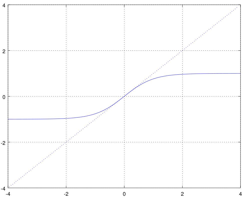 Figure 1
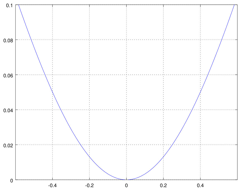 Figure 2
| Type | #input | #output | #hidden | #training | #parameters | #constraints |
|---|---|---|---|---|---|---|
| A | ||||||
| B | ||||||
| C |
| Algorithm | Init. | size class | size class | size class | |||
|---|---|---|---|---|---|---|---|
| #iter. | #iter. | #iter. | |||||
| SVD | — | — | — | — | |||
| SGD | Random | ||||||
| RMSprop | Random | ||||||
| Adadelta | Random | ||||||
| CG | Random | — | — | ||||
| SGD | SVD | ||||||
| RMSprop | SVD | ||||||
| Adadelta | SVD | ||||||
| CG | SVD | — | — | ||||
Peer Reviews
No public reviews on file for this paper yet. If you reviewed it on a platform where reviews are public (OpenReview, ICLR, NeurIPS, ICML), you can paste yours below so the community can read it here.
Videos
No videos yet. Explain this paper in a talk, walkthrough, or lecture? Add one.
11institutetext: Chair of Data Science, Institute of Computer Science
University of St.Gallen, St.Gallen, Switzerland
11email: {bernhard.bermeitinger,tomas.hrycej,siegfried.handschuh}@unisg.ch 22institutetext: University Passau, Passau, Germany
22email: {bernhard.bermeitinger,siegfried.handschuh}@uni-passau.de
Singular Value Decomposition and Neural Networks
Bernhard Bermeitinger 1122 0000-0002-2524-1850
Tomas Hrycej 11
Siegfried Handschuh 1122
Abstract
Singular Value Decomposition (SVD) constitutes a bridge between the linear algebra concepts and multi-layer neural networks—it is their linear analogy. Besides of this insight, it can be used as a good initial guess for the network parameters, leading to substantially better optimization results.
Keywords:
Singular Value Decomposition Neural Network Deep Neural Network Initialization Optimization Conjugate Gradient
1 Motivation
The utility of multi-layer neural networks is frequently being explained by their capability of extracting meaningful features in their hidden layers. This view is particularly appropriate for large size applications such as corpus-based semantics analyses where the number of training examples is too low for making the problem fully determined in terms of a direct mapping from the input to the output space.
This capability of feature extraction is mostly implicitly attributed to using nonlinear units in contrast to a linear mapping. The prototype of such linear mapping is linear regression, using multiplication of an input pattern by a regression matrix to get an estimate of the output pattern, omitting the possibility of using a sequence of two (or more) matrices corresponding to the use of a hidden layer of linear units. This possibility is usually considered to be obsolete with the argument that a product of two matrices is also a matrix and the result is thus equivalent to using a single matrix.
This argument, although superficially correct, hides the possibility of using a matrix of deliberately chosen low rank, which leads to the correct treatment of under-determined problems.
A key to understanding the situation is Singular Value Decomposition (SVD). In the following, it will be shown that SVD can be interpreted as a linear analogy of a neural network with one hidden layer and that it can be used for generating a good initial solution for optimizing nonlinear multi-layer neural networks.
2 Singular Value Decomposition
SVD is a powerful concept of linear algebra. It is a decomposition of an arbitrary matrix of size into three factors:
[TABLE]
where and are orthonormal and is of identical size as , consisting of a diagonal matrix and a zero matrix. For , it is , for it is . In the further discussion, only the case of will be considered as the opposite case is analogous.
SVD is then simplified to
[TABLE]
by omitting redundant zero terms. This form is sometimes called economical.
For the economical form (2), the decomposition with has nonzero parameters. The orthonormality of and imposes unity norm constraints, and orthogonality constraints, resulting in a total number of
[TABLE]
constraints.
The number of free parameters amounts to
[TABLE]
which is
[TABLE]
and, analogically,
[TABLE]
So, the economical form of SVD possesses the same number of free parameters as the original matrix .
The number of nonzero singular values in is equal to the rank of matrix . An interesting case arises if the matrix is not full rank, that is, if . Then, some diagonal elements of are zero. Reordering the diagonal elements of (and, correspondingly the columns of and ) so that its nonzero elements are in the field and zero elements in , the decomposition further collapses to
[TABLE]
Then, with the help of orthogonality of and , the matrix can be decomposed into the sum
[TABLE]
An important property of SVD is its capability for a matrix approximation by a matrix of lower rank. In analogy to the partitioning the singular values with the help of and to nonzero and zero ones, they can be partitioned to large and small ones. Selecting the largest singular values makes (8) to an approximation of matrix . This approximation has the outstanding property of being that with the minimum matrix norm of the difference
[TABLE]
out of all matrices of rank .
The matrix norm of is defined as an induced norm by the vector norm, so that it is defined as
[TABLE]
In many practical cases, a relatively small number leads to approximations very close to the original matrix. Equation 8 shows that this property can be used for an economical representation of a matrix by only numerical values. The optimum approximation property is shown below to be relevant for the mapping approximation discussed below.
A further important application of SVD is an explicit formula for a matrix pseudo-inverse. Pseudo-inverse is the analogy of an inverse matrix for the case of non-square matrices, with the property
[TABLE]
It can be easily computed with the help of SVD:
[TABLE]
with being a matrix of the same dimension as with inverted non-zero elements on the diagonal.
3 SVD and Linear Regression
One of the applications of the pseudo-inverse (11) is a computing scheme for least squares. The linear regression problem is specified by input/output column vector pairs , seeking the best possible estimates
[TABLE]
in the sense of least squares.
The bias vector can be received by extending the input patterns by a unity constant. For simplicity, it will be omitted in the ongoing discussion.
The solution amounts to solving the equation
[TABLE]
with matrices and made of the corresponding column vectors. The optimum is found with the help of the pseudo-inverse of . In the over-determined case (typical for linear regression), the least squares solution is
[TABLE]
In the under-determined case, there is an infinite number of solutions with zero approximation error. The following solution has the minimum matrix norm of :
[TABLE]
Both (15) and (16) use the pseudo-inverse that can be easily computed with help of SVD according to (12).
4 SVD and Mappings of a Given Rank
Both the full SVD (1) and its reduced rank form (7) are products of a dense matrix , a partly or fully diagonal matrix , and a dense matrix . This suggests the possibility of viewing them as a product of two dense matrices and , or and . All these matrices are full rank, even if the original matrix was not due to the under-determination.
The product and is the sequence of two linear mappings. The latter matrix maps the -dimensional input space to an intermediary space of dimension , the former the intermediary space to the -dimensional output space. Since and , the intermediary space represents a bottleneck similar to a hidden layer of a neural network. The orthogonal columns of can be viewed as hidden features compressing the information in the input space. This relationship to neural networks be followed in Section 5.
The reasons to search for such a compressed mapping are different for the over-determined and the under-determined problems.
4.1 Over-determined Problems
Suppose for an over-determined problem with input matrix and output matrix , the best linear solution is sought. The columns of and correspond to the training examples. The least-square-optimum solution is the linear regression
[TABLE]
with matrix from (15). The bias vector can be received by extending the matrix by a unit row and applying the pseudo-inversion of such an extended matrix. The last column of such an extended regression matrix corresponds to the column bias vector .
The linear regression matrix is for input dimension and output dimension , its SVD is as in (1).
With more than independent training examples, the regression matrix and also the matrix are full rank with singular values on the diagonal of .
There may be reasons for assuming that there are random data errors, without which the rank of would not be full. This would amount to the assumption that some of the training examples are, in fact, linearly dependent or even identical and only the random data errors make them different. To ensure correct generalization, it would then be appropriate to assume a lower rank of the regression matrix. This will suggest using the approximating property of SVD with a reduced singular value set. Leaving out the components with small singular values may be equivalent to removing the data noise. Taking a matrix with largest singular values while zeroing the remaining ones (see, e.g., [5]) results in a matrix according to (7):
[TABLE]
that has the least matrix norm
[TABLE]
out of all existing matrices with rank . The matrix norm is induced by the vector norm, as defined in Equation 10. The definition (10) of the matrix norm has an implication for the accuracy of the forecasts with help of and :
[TABLE]
The vector norm of the forecast error equal to the square root of the mean square error is obviously minimal for a given norm of the input vector. In other words, the modified, reduced-rank regression matrix has the least maximum forecast deviation from the original regression matrix relative to the norm of the input vector .
4.2 Under-determined Problems
A different situation is if the linear regression is under-determined. This is frequently the case in high-dimensional applications such as computer vision and corpus-based semantics—the number of training examples may be substantially lower than the dimensions of the input. The training examples span a subspace of the input vector space. Using this training information, new patterns can only be projected onto this subspace. The projection operator, using the same definition of the input matrix as above, is given as:
[TABLE]
This can be viewed as a pattern-specific weighting of training examples by a weight vector
[TABLE]
To recall the corresponding output, the same weight vector can be used:
[TABLE]
This is equivalent to solving the regression problem
[TABLE]
with help of the pseudo-inverse (see, e.g., [3]) of X, which is (16) in the under-determined case.
The regression matrix is, as usual, of size . If the input dimension exceeds the number of training examples the regression matrix solving Equation 24 is not full rank. Its SVD will exhibit some zero singular values and can be reduced, without a loss of information, to a reduced form:
[TABLE]
5 SVD and Linear Networks
Before establishing the relationship between SVD and nonlinear neural networks, let us consider hypothetical multi-layer networks with linear units of the form in the hidden layer.
Suppose a network with one hidden layer of predefined size is used to represent a mapping from input to output . Suppose now that the best linear mapping from input to output is
[TABLE]
The best approximation with a rank limitation to and is, according to (7):
[TABLE]
This expression can be viewed as a network with one linear hidden layer of width . The weight matrix between the input and the hidden layers is
[TABLE]
and that between the hidden and the output layers is
[TABLE]
This network has the property of being the best approximation of the mapping from the input to the output between all networks of this size with orthonormal (in the hidden layer) and orthogonal (in the output layer) weight vectors.
This optimality is not strictly guaranteed to be reached if relaxing the orthogonality constraints. The difference between the orthogonal and the non-orthogonal solutions depends on the ratio between the input and the output widths, and on the relative width of the hidden layer in the following way.
How serious this optimality gap may be can be assessed observing the fraction of the number of orthogonality constraints to the number of parameters. If this fraction is small, the number of independent parameters is close to the number of all parameters and the influence of the orthogonality constraints is small.
With hidden layer size (equal to the rank of the linear mapping), the total number of constraints is . With and , the total number of parameters is . The fraction, and its approximation for realistic values of is then
[TABLE]
This fraction decreases with the ratio (the degree of feature compression by the network) and the ratio . Since both ratios will usually be large in practical problems of the mentioned domain, the distance to the optimality after relaxing the orthogonality constraints can be expected to be small.
6 SVD and Initializing Nonlinear Neural Networks
Most popular hidden units possess a linear or nearly linear segment. A sigmoid unit
[TABLE]
is nearly linear around the point where its derivative is equal to . Rescaling this unit to the symmetric form
[TABLE]
we obtain a nonlinear function the derivative of which is unity around , plotted in Figure 1.
Its relative deviation from the linear function is below ten percent for (see Fig. 2). So, a neural network with one hidden layer using the sigmoid activation function (32) behaves like a linear network for small activation values of the hidden layer.
This fact can be used for finding a good initial guess of parameters of a nonlinear neural network with a single hidden layer. The in-going weights into the hidden and output layers are (28) and (29), respectively.
7 Computing Experiments
A series of computing experiments have been carried out to assess the real efficiency of using SVD as a generator of the initial state of neural network parameters. To provide a meaningful interpretation of the mean square figures attained, all problems have been deliberately defined to have a minimum at zero. To justify the use of the hidden layer as a feature extractor, its width should be smaller than the minimum of the input and output sizes. The dimensions have been chosen so that the full regression would be under-determined (as typical for the application types mentioned above), but the use of a hidden layer with a smaller width makes it slightly over-determined. So, the effect of overfitting, harmful for generalization, is excluded.
The software used for SVD computation was the Python module SciPy [2]. Neural networks were optimized by several methods implemented in the popular framework Keras [1]: Stochastic Gradient Descent (SGD), selected because of its widespread use, as well as Adadelta and RMSprop, which seem to be the most efficient ones for the problems considered.
Typical Keras-methods are first order and there is a widespread opinion in the neural network community that second-order methods are not superior to the first order ones. However, there are strong theoretical and empirical arguments in favor of the second-order methods from numerical mathematics. So the conjugate gradient method (CG), as implemented in SciPy, has also been applied. Since the SciPy/Keras interface failed to work for this method111Since we use TensorFlow as Keras’ backend execution engine, the resulting computation graph would have been cut into two different executions for each optimization step which causes a too high computational overhead., efficient Keras-based network evaluation procedures could not be used. So, for the largest problems, the CG method had to be omitted.
The performance of the optimization methods has been compared with the help of the number of gradient calls. All methods have been used with the default settings of Keras and SciPy.
Three problem sizes denoted as , , and have been used. Using different size classes will make it possible to discern possible dependencies on the problem size if there are any. The largest size of class is still substantially below that of huge networks such as VGG-19 [4] used in image classification. The computing effort for making method comparison with such huge sizes would be excessive for the goals of this study. However, we believe the size is sufficient for showing trends relevant for very large network sizes.
The three size classes are characterized by their input and output dimensions as well as by the size of the training set. The concrete network sizes, parameter numbers, and numbers of constraints (output values to be reached times the number of training examples) are given in Table 1. The column “# constraints” shows the number of constraints imposed by the reference outputs to be fitted. It is the product of the output dimension and the training set size. Comparing the number of constraints with the number of parameters defines the over-determination or the under-determination of the problem (e.g., a problem with more constraints than parameters is over-determined).
The results for the different size classes are given in Table 2. For each network architecture, three different parametrizations with corresponding training sets have been generated, all with a known mean square error minimum of zero. For every variant, an SVD has been computed and used to determine the network initialization. For comparison, five different random network initializations have been generated. The results below are geometric means of minima reached (means from three optimization runs for SVD initializations, and means from runs for random initializations).
The results of four optimization methods are given in the randomly initialized variant and in the variant initialized with help of the SVD solution.
The first row, labeled with algorithm “SVD”, shows the minima reached by the SVD solution without any subsequent optimization. It is obvious that the SVD-based initialization is pretty good. Its mean square error minimum is substantially better than the weakest Keras-method SGD with random initialization. For the largest problem size class, SVD without optimization is also superior to Adadelta with random initialization.
An SVD-based initialization with a subsequent optimization lets SGD reach an acceptable minimum, with even better results using Adadelta. The best Keras-method, RMSprop, was clearly inferior to the conjugate gradient (CG), although CG stopped the optimization substantially earlier that the fixed iteration number of RMSprop. For both these methods, the improvement by SVD-based initialization was weak (for CG only in the number of iterations). This is not unexpected: good optimization methods are able to find the representations similar to the SVD by themselves, solving a closely related problem with a different numerical procedure.
8 Conclusion and Discussion
SVD constitutes a bridge between the linear algebra concepts and multi-layer neural networks—it is their linear analogy. Besides this insight, it can be used as a good initial guess for the network parameters. The quality of this initial guess may be, for large problems, better than weakly performing (but widely used) methods such as SGD ever reach.
It has to be pointed out that as long as the network uses nonlinear hidden units, simply using this initial guess as ultimate network parameters makes little sense: it would be preferable to make the units linear, and use the SVD matrices directly to represent the desired input-output mapping.
Unfortunately, there seems to be no analogous generalization for networks with multiple hidden layers. With a hidden layer sequence of monotonically decreasing width (for example, from the input towards the output) it would be possible to proceed iteratively, by successively adding hidden layers of decreasing width.
The procedure would start by defining the first hidden layer (the one with the largest dimension) and initializing its weights with the help of SVD. Then, the following iterations over the desired number of hidden layers would be performed:
Analyzing the mapping between the output of the last hidden layer considered and the output layer (with ) using SVD. 2. 2.
Finding an initial guess of parametrization for the incoming weights to . 3. 3.
Optimizing the weights of such extended nonlinear network by some appropriate optimization method.
This is a formal generalization of the procedure for the network with a single hidden layer , as presented above.
However, it is difficult to find a founded justification for this procedure, as it is equally difficult to find a founded justification for using multiple fully connected hidden layers at all—although there seems to be empirical evidence in favor of this. Of course, there are good justifications for using special architectures such as convolutional networks, which are motivated, e.g., by spatial operators in image processing.
The reference list from the paper itself. Each links out to its DOI / PubMed record.
- 1[1] Chollet, F., others: Keras (2015), https://keras.io
- 2[2] Jones, E., Oliphant, T., Peterson, P., others: Sci Py: Open source scientific tools for python (2001), http://www.scipy.org/
- 3[3] Kohonen, T.: Self-Organization and Associative Memory. Springer Series in Information Sciences, Springer-Verlag, 3 edn. (1989), https://www.springer.com/de/book/9783540513872
- 4[4] Simonyan, K., Zisserman, A.: Very deep convolutional networks for large-scale image recognition. ar Xiv 1409.1556 (09 2014), http://arxiv.org/abs/1409.1556
- 5[5] Trefethen, L.N., Bau III, D.: Numerical linear algebra, vol. 50. Siam (1997)