A Constant-Factor Approximation Algorithm for Online Coverage Path Planning with Energy Constraint
Ayan Dutta, Gokarna Sharma

TL;DR
This paper presents a constant-factor approximation algorithm for energy-constrained coverage path planning in unknown environments, ensuring efficient exploration with bounded path length and obstacle avoidance.
Contribution
It introduces an $O(1)$-approximation algorithm for coverage with energy constraints, improving upon previous logarithmic approximation methods.
Findings
Algorithm achieves constant-factor approximation guarantee.
Outperforms existing algorithms in path length and runtime.
Effective in environments with various obstacle shapes.
Abstract
In this paper, we study the problem of coverage planning by a mobile robot with a limited energy budget. The objective of the robot is to cover every point in the environment while minimizing the traveled path length. The environment is initially unknown to the robot. Therefore, it needs to avoid the obstacles in the environment on-the-fly during the exploration. As the robot has a specific energy budget, it might not be able to cover the complete environment in one traversal. Instead, it will need to visit a static charging station periodically in order to recharge its energy. To solve the stated problem, we propose a budgeted depth-first search (DFS)-based exploration strategy that helps the robot to cover any unknown planar environment while bounding the maximum path length to a constant-factor of the shortest-possible path length. Our -approximation guarantee advances the…
Click any figure to enlarge with its caption.
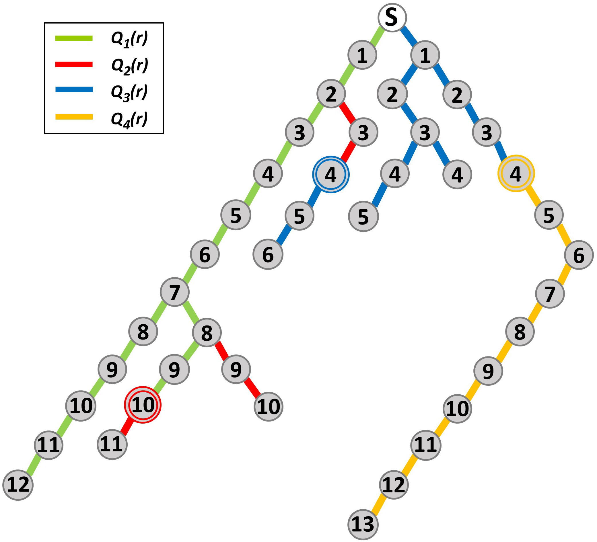 Figure 1
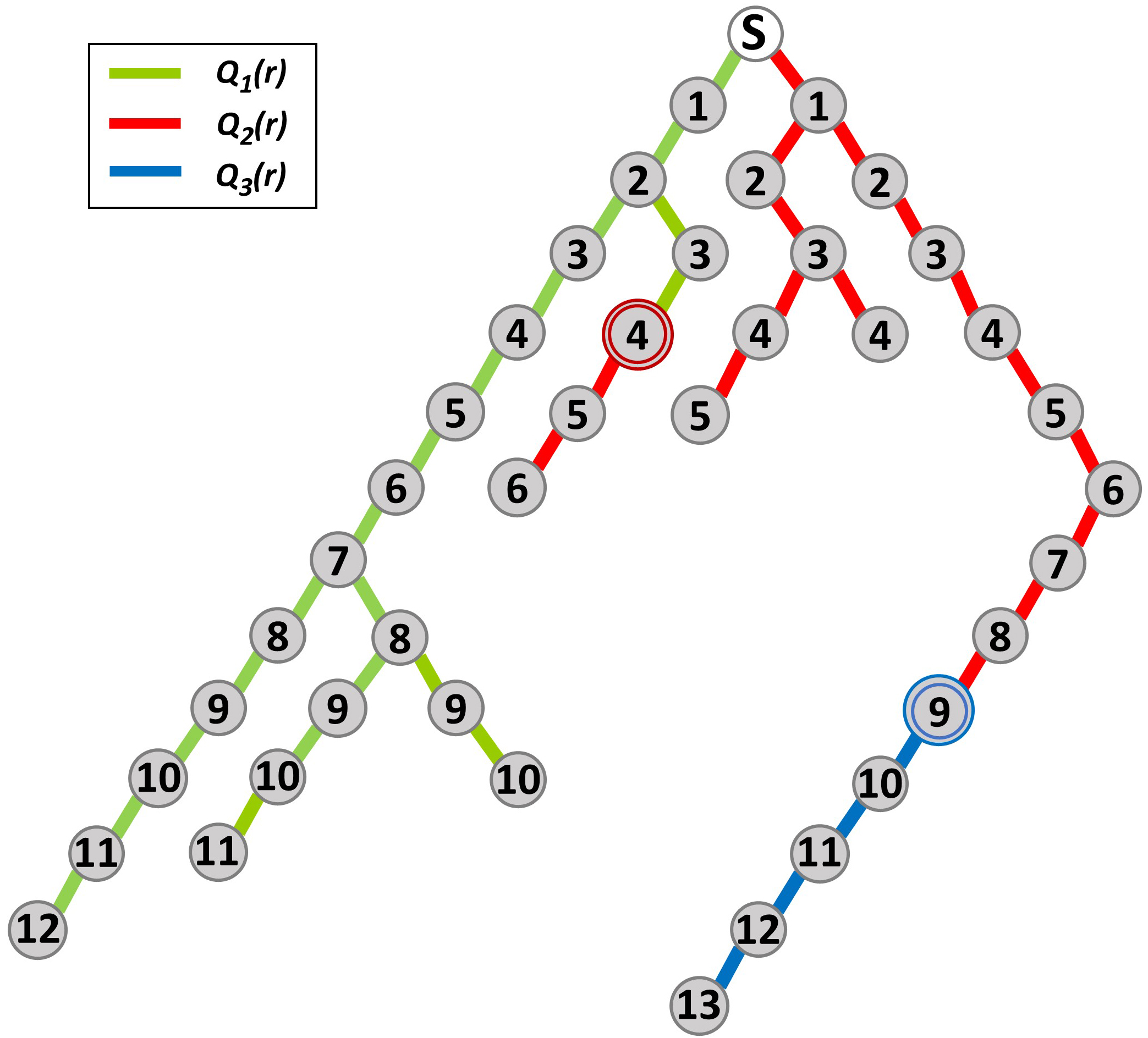 Figure 2
 Figure 3
 Figure 4
 Figure 5
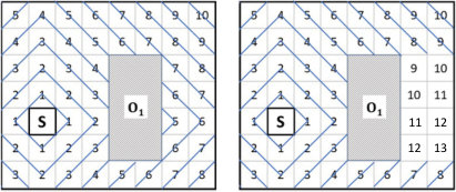 Figure 6
 Figure 7
 Figure 8
 Figure 9
 Figure 10
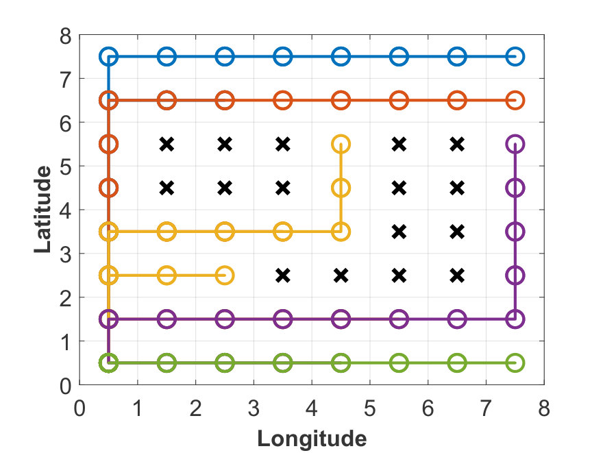 Figure 11
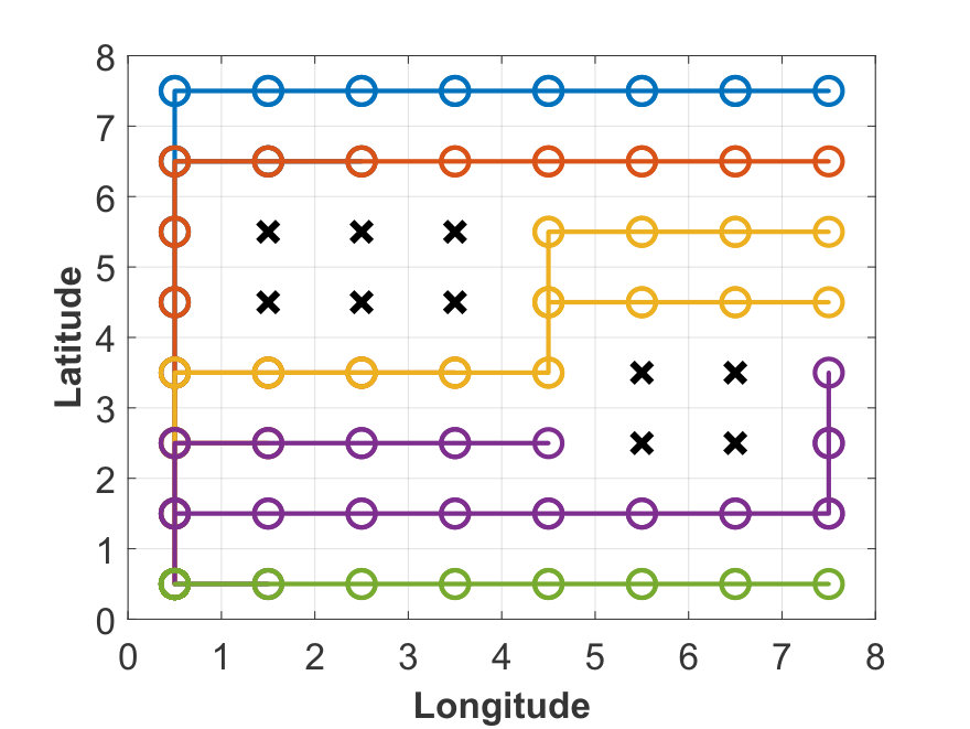 Figure 12
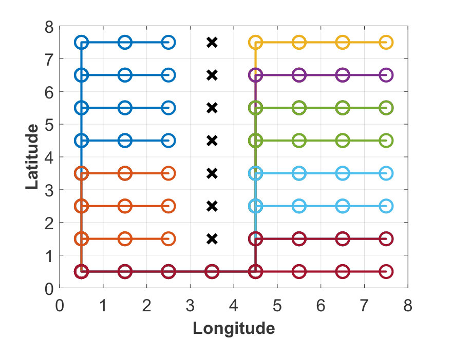 Figure 13
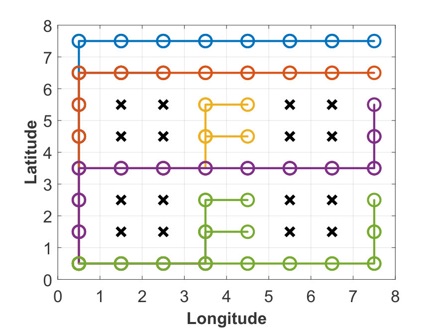 Figure 14
 Figure 15
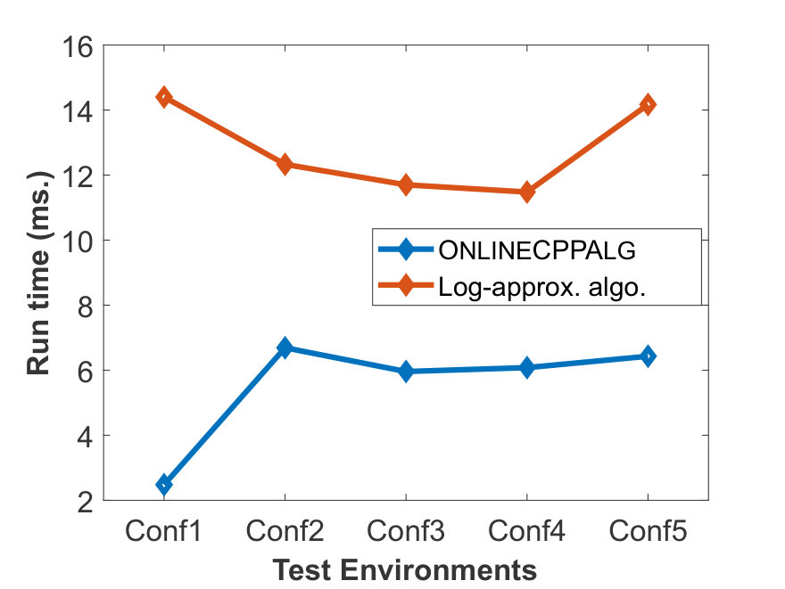 Figure 16
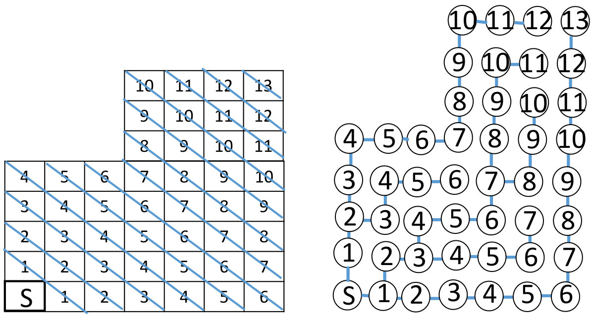 Figure 17
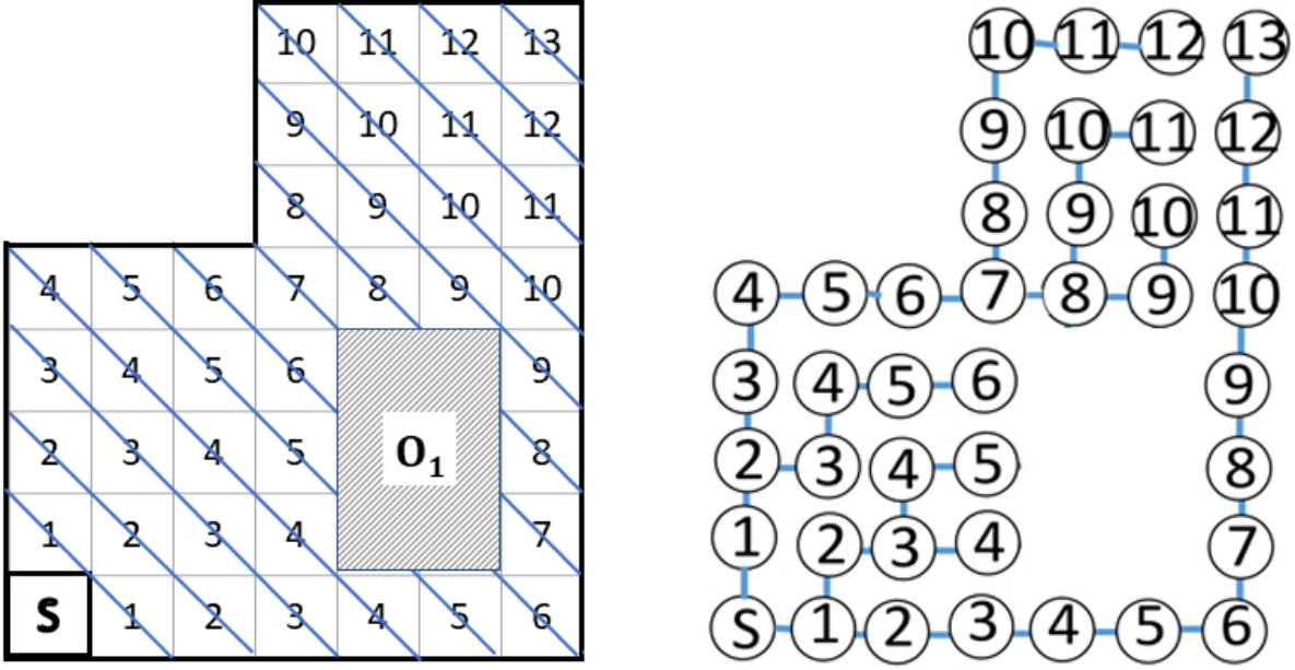 Figure 18
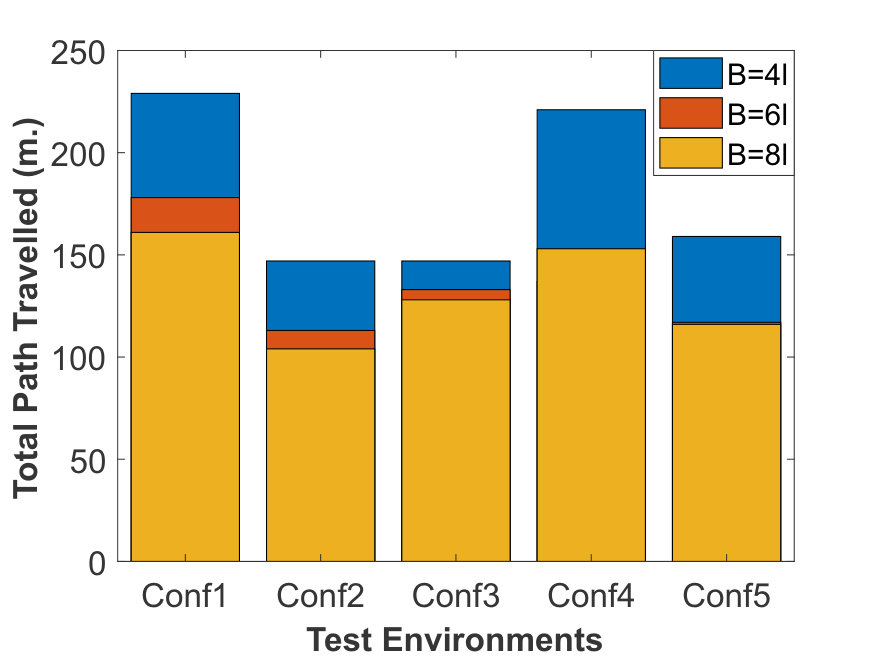 Figure 19
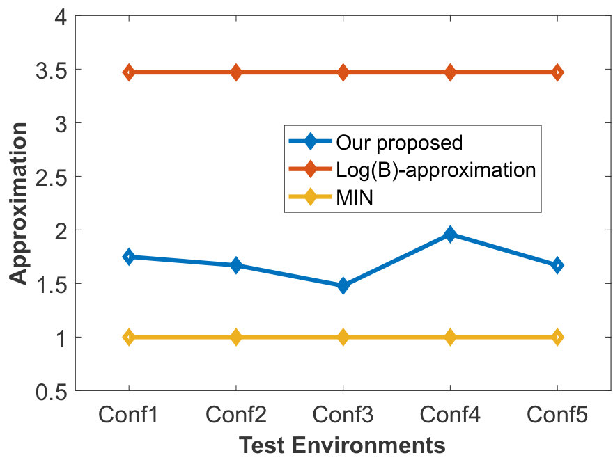 Figure 20
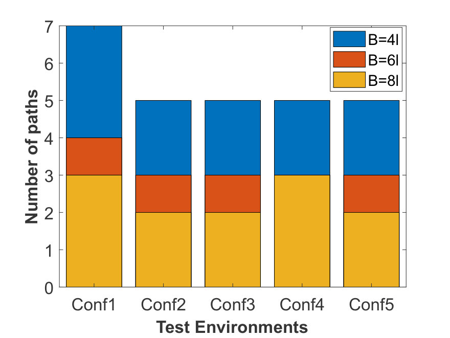 Figure 21
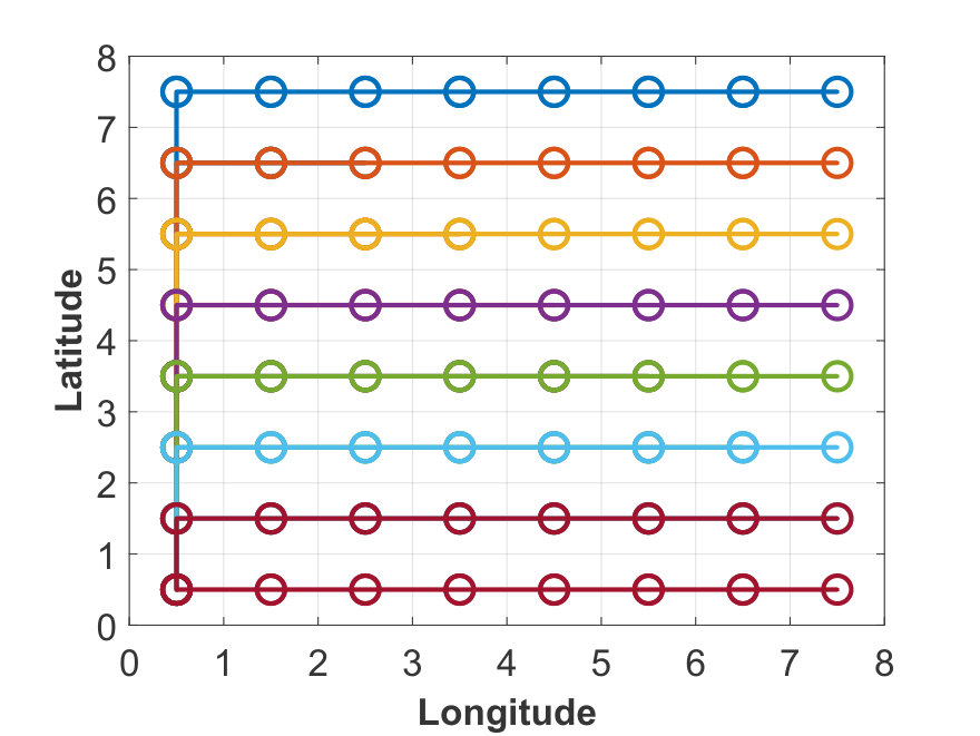 Figure 22
 Figure 23
 Figure 24
 Figure 25
 Figure 26
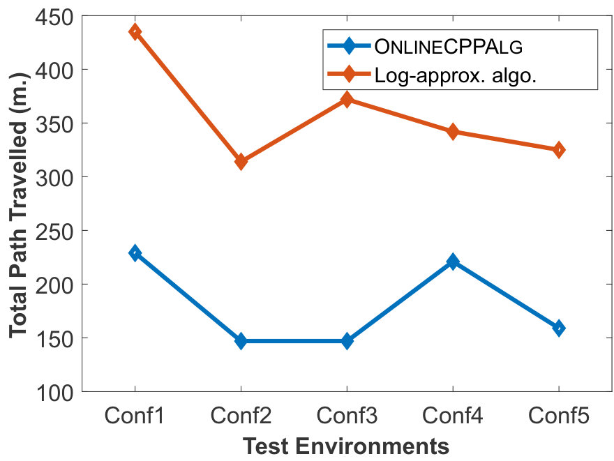 Figure 27
 Figure 28
 Figure 29
 Figure 30
Peer Reviews
No public reviews on file for this paper yet. If you reviewed it on a platform where reviews are public (OpenReview, ICLR, NeurIPS, ICML), you can paste yours below so the community can read it here.
Videos
No videos yet. Explain this paper in a talk, walkthrough, or lecture? Add one.
Taxonomy
TopicsRobotic Path Planning Algorithms · Optimization and Search Problems · Vehicle Routing Optimization Methods
A Constant-Factor Approximation Algorithm for Online
Coverage Path Planning with Energy Constraint
Ayan Dutta, Gokarna Sharma A. Dutta is with the School of Computing, University of North Florida, Jacksonville, FL 32224, USA [email protected]. Sharma is with the Department of Computer Science, Kent State University, Kent, OH 44242, USA [email protected]
Abstract
In this paper, we study the problem of coverage planning by a mobile robot with a limited energy budget. The objective of the robot is to cover every point in the environment while minimizing the travelled path length. The environment is initially unknown to the robot. Therefore, it needs to avoid the obstacles in the environment on-the-fly during the exploration. As the robot has a specific energy budget, it might not be able to cover the complete environment in one traversal. Instead, it will need to visit a static charging station periodically in order to recharge its energy. To solve the stated problem, we propose a budgeted depth first search (DFS)-based exploration strategy that helps the robot to cover any unknown planar environment while bounding the maximum path length to a constant-factor of the shortest-possible path length. Our -approximation guarantee advances the state-of-the-art of log-approximation for this problem. Simulation results show that our proposed algorithm outperforms the current state-of-the-art algorithm both in terms of the travelled path length and run time in all the tested environments with concave and convex obstacles.
I Introduction
Coverage planning is the task of finding a path or a set of paths to cover all the points in an environment [5]. In robotics, this problem has many potential real-world applications including autonomous sweeping, vacuum cleaning, and lawn mowing. In an online version of the problem, the area of interest is initially unknown to the robot. Therefore it needs to discover and avoid the unknown obstacles in the environment while covering all the points in the free space by traveling as minimum distance as possible [5].
Traditionally, this problem has been studied assuming that the robot has an unlimited energy budget, where given a robot, a single path can be planned to cover the given environment. The offline version of the problem where the robot(s) have a priori knowledge of the environment including obstacles has been well studied, e.g., see [9]. Many algorithms have been proposed such as the boustrophedon decomposition based coverage [4, 13], the spiral path coverage [10], and the spanning-tree based coverage [8]. These techniques can also be adapted to solve online coverage planning [20, 3].
In practice however, the robots do not have unlimited energy available. Therefore, even covering a standard-size environment (e.g., a farm) while simultaneously using on-board sensors (e.g., camera) becomes prohibitive with a single charge. A battery-powered robot needs to return to the charging station to get recharged before the battery runs out. Due to practical relevance, in the recent years, there has been a significant volume of work on the energy-constrained coverage planning problem [18, 14, 20, 19, 17, 16]. The offline version of the problem, denoted as OfflineCPP, is studied in [17, 20, 19] and the online version, denoted as OnlineCPP, is studied in [16, 17]. The state-of-the-art algorithm for OfflineCPP is due to [19], which provides -approximation. For OnlineCPP, the state-of-the-art algorithm is due to [16], which provides -approximation, where is the energy budget and is the size of the robot (assuming a square robot). Our goal in this paper is to provide a better approximation algorithm for OnlineCPP, i.e., to reduce the -approximation of [16] to . This will show that asymptotically there is no approximation gap between OnlineCPP and OfflineCPP.
Our proposed algorithm covers an unknown environment through a DFS traversal approach tailored for the limited energy budget . Robot performs a depth first search traversal while building a tree map of the environment on-the-fly. It returns to the charging station to get its battery fully recharged (stopping the DFS exploration) when the path length of the traversal becomes at most . After the battery is fully charged, then moves to the cell where it stopped the DFS process, and continues traversing . Simulation results show that our proposed algorithm is up to times faster and up to times less costlier (in terms of traversed path length) than the state-of-the-art algorithm [16].
Contributions. Initially, the robot is at the charging station that is inside . The goal of OnlineCPP is to find a set of paths for the robot such that
- •
Condition (a): Each path starts and ends at
- •
Condition (b): Each path has length
- •
Condition (c): The paths in collectively cover the environment , i.e., ,
and the following two performance metrics are optimized:
- •
Performance metric 1: The number of paths in , denoted as , is minimized, and
- •
Performance metric 2: The total lengths of the paths in , denoted as , is minimized.
We establish the following main theorem for OnlineCPP.
Theorem 1** (Main Result)**
Given an unknown planar polygonal environment possibly containing obstacles and a robot of size consisting of position and obstacle detection sensors initially situated at a charging station inside with energy budget , there is an algorithm that correctly solves OnlineCPP and guarantees -approximation to both performance metrics compared to the optimal algorithm that has complete knowledge about .
This result clearly advances the current state-of-the-art as it improves upon the log-approximation provided in [16] and provides a constant-factor approximation. Furthermore, the proposed algorithm is easier to implement than [16].
Related Work. The most closely related works to ours are [16, 20, 19, 17]. Shnaps and Rimon [17] proposed an -approximation algorithm for OfflineCPP, where is the ratio between the furthest distance between any two cells in the environment and half of the energy budget [17]. For OnlineCPP, they proposed an -approximation algorithm. Wei and Isler [20] presented an -approximation algorithm for OfflineCPP, which has been improved to a constant-factor approximation by them in [19]. Recently, Sharma et al. [16] provided an -approximation algorithm for OnlineCPP. In this paper, we improve upon the log-approximation bound and provide the -approximation to OnlineCPP.
The other related work is the coverage of a graph. The goal is to design paths to visit every vertex of the given graph. Without energy constraints, it becomes the well-known Traveling Salesperson Problem (TSP) [1] and a DFS traversal provides a constant-approximation of the TSP. With energy constraints, this coverage problem becomes the Vehicle Routing Problem (VRP) [11]. One version of VRP is the Distance Vehicle Routing Problem (DVRP), which models the energy consumption proportional to the distance travelled. For DVPR on tree metrics, Nagarajan and Ravi [15] proposed a 2-approximation algorithm. Li et al. [12] used a TSP-partition method and their algorithm has a similar approximation to the work in [17]. Most of these work studied the offline version so that pre-processing on the environment can be done prior to exploration obtaining better approximation. This is also the case in the algorithm of [20, 19] for OfflineCPP. Coverage with multiple robots has also received a lot of attention (e.g., see [2, 7]). In some cases, the paths planned for a single robot under energy constraints can also be executed by multiple robots by assigning the planned paths to the robots, without affecting the total cost. In this paper, we consider coverage planning with a single robot.
II Problem setup
In this paper, we use the same model as in [16, 20, 17].
Environment. The environment is a planar polygon containing a single charging station inside it. may possibly contain polygonal, static obstacles. See left of Fig. 1 for an illustration of with an obstacle . The environment is discretized into cells forming a 4-connected grid.
Robot. We consider the robot to be initially positioned at the charging station . has size that it fits within a grid-cell in . The robot moves rectilinearly in , i.e., it may move to any of the four neighbor cells (if the cell is not occupied by an obstacle) from its current cell. We also assume that has the knowledge of the global coordinate system through a compass on-board, that means it knows left (West), right (East), up (North), and down (South) cells consistently from its current cell. Robot is equipped with a position sensor (e.g., GPS) and an obstacle-detection sensor (e.g., laser rangefinder). We assume that with the laser rangefinder, the robot can detect obstacles in any of its neighbor cells. The robot has sufficient on-board memory to store information necessary to facilitate the coverage process. Moreover, we assume that initially does not have any knowledge about , i.e., is an unknown environment. For the feasibility of covering all cells of , we assume that is as big as a circle of radius with center at . It is assumed that the energy consumption of the robot is proportional to the distance travelled, i.e., the energy budget of allows the robot to move units distance.
A path (route) is a list of cells that visits starting and ending with . Notice that if there are some obstacles within located in such a way that they divide into two sub-polygons and with and sharing no common boundary, then cannot fully cover . Therefore, we assume that there is no such cell in . That means, there is (at least) a route from to any obstacle-free cell of .
We call a cell free if it is not occupied by an obstacle. We call a cell reachable if it satisfies the definition below.
Definition 1** (Reachable Cell)**
Any cell in is called reachable by the robot , if and only if (a) it is a free cell, (b) it is within distance from , and (c) there must be at least a route of consecutive free cells from to .
OnlineCPP**.** The problem is formally defined as follows.
Definition 2
Given an unknown planar polygonal environment possibly containing obstacles with a robot having battery budget of initially positioned at a charging station inside , OnlineCPP is for to visit all the reachable cells of through a set of paths so that
- •
Conditions (a)–(c) are satisfied, and
- •
Performance metrics (1) and (2) are minimized.
Following [16, 19], we measure the efficiency of any algorithm for OnlineCPP in terms of approximation ratio which is the worst-case ratio of the cost of the online algorithm for some environment over the cost of the optimal, offline algorithm for the same environment.
III Processing Unknown Environment
In this section, we discuss how the robot decomposes the environment into square grid cells and then construct a tree map of the environment on-the-fly.
Decomposition of the Environment.
Following [16, 19], we decompose the environment into square cells of size , which is the size of the robot itself.
An equi-distance contour is a poly-line where the cells on it has the same distance to/from the base point (the left of Fig. 1). The cells on a contour can be ordered from one side to the other.
Let be a cell and be a contour. Let denote the distance to from and let denote the distance to from . If , we say that contour is contour ’s next contour. The contour with is called the first contour. Each cell in a contour has at most reachable cells from that are its neighbors.
Constructing a Tree Map.
Initially, the robot is placed at the fixed charging station . In this case, the tree, denoted by , has only one node , which we call the root of . If there is no obstacle in , each cell except the boundary cells of will have exactly four neighbor cells.
Robot picks the first free cell according to a clockwise ordering of its neighbors starting from the west and ending in the south neighbor cell. then inserts it into as a child of . If the cell labeled West is a reachable cell, then picks that cell. Otherwise, it goes in order of North, East, and South until it finds the first cell that is reachable. We now have two nodes in , with as a child node of . Furthermore, is a cell in the first contour .
Since is building while exploring , it will move to after it is included as a child in . The robot then again repeats the process of building from its current cell . While at , is only allowed to add one of the neighboring cells of that are in the second contour (i.e., ) as a child of . For this, will include a neighboring cell of in only if is a cell in contour . Furthermore, if some cell is already a part of , then this cell will not be included in again. This process will then continue. The right of Fig. 1 provides an illustration of the tree map developed for the environment shown on the left.
Essentially, any edge of connects two cells of such that and , for ; in Fig. 1, each cell of contour on the environment on the left are at depth in shown on the right. Therefore, using this approach, all the cells in the first contour will be children of (the root of ), all the cells in the second contour will be children of the nodes of that are cells in the first contour , and so on.
There is one potential problem in certain situations. Consider the environment shown in Fig. 2 where the horizontal line passing through is crossing obstacle . The contour numbering and constructing based on contour numbers do not work as the cells in the right of may not be visited by following Algorithm 1 as it requires the robot to visit the cells in an increasing order of contour numbers. This is because the contour numbers for those cells are smaller than the contour number of the cells on North, South, and West of the obstacle. For example, see the left of Fig. 2.
We solve this problem in Algorithm 1 using an approach where the robot detects this problem and changes the contour numbers of those cells on-the-fly. See for example the right of Fig. 2 that depicts how the contour numbers for the cells on the right of are updated on-the-fly by the robot. Details are omitted on how detects the problem and solves it due to space constraints.
IV Algorithm
In the description of the algorithm and its analysis, we assume that . A simple adaptation will work when . The pseudocode is given in Algorithm 1 and illustration of the working principle of the algorithm is given in Fig. 3.
IV-A A Naive Approach without Energy Constraint
The main idea behind our algorithm is to let incrementally explore the environment while simultaneously constructing a tree map of to keep track of the new frontiers that need to be visited by it.
For simplicity, let us first consider that (or ) is known a priori and has no energy constraint (i.e., ). Let be a route in that visits all the nodes of , obtained performing a Depth First Search (DFS) traversal of . Since is a tree, it is known that all the nodes of can be covered by the DFS traversal by visiting each node of at most twice. Therefore, if there are nodes in , then the length of the route . Moreover, an optimal algorithm for to traverse all nodes of must have length , since can only visit the nodes of sequentially one after another using any algorithm. Therefore, without any energy constraint (), we have a -approximation algorithm. The 2-approximation can also be guaranteed for OnlineCPP when since with the knowledge of the global coordinate system, can visit all the nodes of as if is known a priori, satisfying the length of the route .
IV-B Incorporating the Energy Constraint
Now suppose that has energy budget . The aforementioned algorithm is not sufficient anymore since each route of can be at most of length . Therefore, needs to return to to get recharged before the length of the robot’s path reaches . Our proposed algorithm uses the same idea of performing a DFS traversal of as described in the previous subsection while stopping the DFS traversal process before the route of has length at most . Let be the route with respective nodes visited by while running DFS assuming . Let denote a route of visiting the nodes of when . The goal is to obtain , such that the three conditions listed in Section I are satisfied.
The challenge is to plan each route in an online fashion satisfying all three criteria while minimizing both the number of paths and the total length of the paths . We use the following approach: starts from and visits the nodes of in a sequence. As soon as reaches to a node such that , it terminates the DFS traversal and returns to . is the energy remained after each move. In route , moves to (where it stopped the DFS traversal in ) from and continues the DFS traversal until it reaches to a node from which . Like last route, then returns to . This process then continues until the last node is visited in some route . We later prove that using this approach, visits all nodes of providing correctness and approximation guarantee claimed in Theorem 1.
We call our algorithm OnlineCPPAlg (shown in Algorithm 1). Initially, the robot is at with the energy budget . This is a special situation where and . Robot then includes the child nodes of (in contour 1) in making them child nodes of root in and moves to the leftmost child node, say . The node is marked visited. is decreased by 1 (line ). Robot then moves from to the leftmost child node (in contour 2). The node is marked visited and is decreased by 1. This process continues until at some node (in some contour ), , where is the distance from to in . Robot then returns to following the path in (line ). After getting fully charged at , follows the path in to reach to continue the DFS traversal.
At any cell of (node of ), if it has a unvisited neighbor cell in the next contour (child node in ), then moves to that cell. Otherwise, retreats back to the parent node cell of its current cell in (lines ). During the exploration, anytime realizes that it has just enough energy remaining to reach back to , it does so by visiting the parent nodes in the tree starting from its current node.
V Analysis of the Algorithm
In this section, we provide theoretical analysis of OnlineCPPAlg. We first prove its correctness and then analyze the costs for the performance metrics (1) and (2).
Correctness. We start with the following lemma.
Lemma 1
Let be the order of the nodes of (i.e., cells in ) visited by the DFS traversal when . Let be the routes of that collectively visit the nodes of at least once when . The not-yet-visited nodes of (or cells of ) are visited in in the same order as in .
Proof:
Consider the paths in when . In this case, instead of stopping the DFS traversal at some node and make a round trip to from , each subsequent paths continue their traversal without this stoppage. This simulates essentially the behavior of when giving and hence the nodes of (or cells in ) are visited in the same order in both (except the nodes visited in the roundtrip to from the stopped node ). ∎
Theorem 2** (Correctness)**
OnlineCPPAlg* completely covers the environment .*
Proof:
When is known a priori, can visit all the reachable cells in with an unlimited budget. If is unknown but , it is also known that through a DFS traversal, each reachable cell of is guaranteed to be visited where the traversal path is represented by . We have proved in Lemma 1 that when is unknown but , the nodes of are visited in the same order. This immediately provides the guarantee that all reachable cells of will be visited by . Hence, proved. ∎
Approximation Ratio. We prove the following theorem.
Theorem 3** (Approximation)**
OnlineCPPAlg* achieves -approximation for both performance metrics – the number of paths and the total lengths of the paths.*
Proof:
Let be a tree of depth at most . Let be a robot with energy budget at least . After starts from to visit the nodes of , due to the limited energy budget, may need to stop the coverage of and visit the charging station again before rest of the nodes in can be covered.
Let be the DFS exploration strategy for that consists of the minimum number of routes, i.e., the minimum number of times needs to visit before is completely covered. Let be the DFS exploration strategy that visits the nodes of (starting from ) using a DFS traversal where length of each route is bounded by . As soon as the battery is fully charged at , in the next route, directly goes to the node of where it stopped the DFS traversal in the last route and continues covering the unvisited nodes of . For any tree of depth and any robot of energy budget at least , we have the following result from [6] on the number of routes , of the strategy , compared to the number of routes , of strategy : . Moreover, let be the total length traversed by while using the strategy . Let be the optimal length traversed by . Again from [6], we have that .
The above results are interesting meaning that the bounds hold for any arbitrary DFS traversal of by . That means that the whole DFS traversal does not need to be known beforehand (i.e., can be computed online not knowing in advance). Moreover, each route can be constructed without any knowledge on the yet unvisited part of .
We now discuss how the two results can be adapted to prove the same bounds for OnlineCPPAlg. Consider a DFS traversal of (or equivalently ) by when . We have from Lemma 1 that the routes in visit the not-yet-visited nodes of in the order same as in . Moreover, the tree map of formed during the exploration is of depth at most . Therefore, and . ∎
Proof of Theorem 1: Theorems 2 and 3 prove Theorem 1 for . Since the cells are decomposed proportional to the robot size , a simple adaptation of the analysis again gives -approximation for OnlineCPPAlg for . The correctness analysis remains unchanged. ∎
VI Evaluation
Settings. We have implemented the proposed algorithm OnlineCPPAlg using Java programming language on a desktop computer with an Intel i7-7700 CPU and 16GB RAM. The robot size is set to . We have created five different environments with both convex and concave obstacles in them. The test environments are of the same dimension – . The budget is set to (unless otherwise mentioned), i.e., four times the size of each side of the environment. Note that this is the lowest possible budget to completely cover the environment. The charging station is placed at the left-bottom corner in every test environment. These environments are shown in Fig. 4 (Conf1 to Conf5).
Empirically, we have mainly focused on three metrics to evaluate the quality of the proposed algorithm: 1) time to cover the environment, 2) total path length traversed by the robot, and 3) approximation ratio. We also compare our results against the current state-of-the-art algorithm that solves OnlineCPP under energy constraint [16].
Results. First we empirically verify the theoretically-proved constant-factor approximation bound. Let denote the number of reachable cells in the environment. Then will indicate the absolute minimum number of paths required by the robot to completely cover the environment [16, 20]. No optimal DFS strategy () can guarantee a better approximation bound than . Here, we compare our experimental result against as a comparison against any cannot make our empirical approximation bound worse. The result is shown in Fig. 5(a). The state-of-the-art bound of (when ) is also plotted for reference. The figure shows that in practice, the approximation bound is well below the -factor theoretical worst-case bound. Also, in all of the test environments, our proposed algorithm outperforms the state-of-the-art -approximation [16].
As we are minimizing the total path length travelled by the robot to completely cover the environment, we are interested to compare this metric for our algorithm against the algorithm in [16]. The result is shown in Fig. 5(b). It can be clearly observed from this plot, that our proposed algorithm outperforms the algorithm in [16] in terms of the travelled path length – by an average ratio of while the maximum ratio is (Conf3).
Next we are interested to investigate the effect of changing the budget amount on the travelled path length. In order to do this, we vary between . The result is shown in Fig. 6(a). With higher budget, could cover more cells in one path than with a lower budget. This fact is also reflected in the plot where travelled path length is higher with lower budget and vice-versa. Similarly, when the budget is higher and is covering more cells in a single path, it needs to come back to the charging station less often and consequently, the total number of paths also reduces. This can be observed in Fig. 6(b). On average, visited times more with than with .
Next we are interested to investigate the run time of the proposed algorithm. We also compare this metric against the algorithm proposed in [16]. The result is shown in Fig. 7. On average, our algorithm is shown to be times faster than [16] while the maximum ratio is (Conf1). Finally, the paths followed by in different environment configurations are shown in Fig. 4; a video of the simulation is also submitted.
VII Conclusion and Future Work
We have presented an algorithm for OnlineCPP by an energy-constrained robot achieving -approximation, improving significantly on the state-of-the-art -approximation [16]. It is also simpler to implement compared to [16]. Our simulation results validate the approximation bound established theoretically. We have empirically shown that our proposed approach outperforms the state-of-the-art algorithm both in terms of run time and total traversal cost for the complete coverage. In the future, we plan to test our algorithm in a real-world setting.
The reference list from the paper itself. Each links out to its DOI / PubMed record.
- 1[1] D. L. Applegate, R. E. Bixby, V. Chvatal, and W. J. Cook. The Traveling Salesman Problem: A Computational Study . Princeton University Press, Princeton, NJ, USA, 2007.
- 2[2] P. Brass, A. Gasparri, F. Cabrera-Mora, and J. Xiao. Multi-robot tree and graph exploration. In ICRA , pages 495–500, 2009.
- 3[3] Y. Choi, T. Lee, S. Baek, and S. Oh. Online complete coverage path planning for mobile robots based on linked spiral paths using constrained inverse distance transform. In IROS , pages 5788–5793, 2009.
- 4[4] H. Choset. Coverage of known spaces: The boustrophedon cellular decomposition. Auton. Robots , 9(3):247–253, Dec. 2000.
- 5[5] H. Choset. Coverage for robotics–a survey of recent results. Annals of mathematics and artificial intelligence , 31(1-4):113–126, 2001.
- 6[6] S. Das, D. Dereniowski, and P. Uznanski. Brief announcement: Energy constrained depth first search. In ICALP , pages 165:1–165:5, 2018 (A full version in http://arxiv.org/abs/1709.10146).
- 7[7] P. Fraigniaud, L. Ga̧sieniec, D. R. Kowalski, and A. Pelc. Collective tree exploration. Netw. , 48(3):166–177, 2006.
- 8[8] Y. Gabriely and E. Rimon. Spanning-tree based coverage of continuous areas by a mobile robot. Annals of Mathematics and Artificial Intelligence , 31(1-4):77–98, May 2001.