$T$-equivariant disc potential and SYZ mirror construction
Yoosik Kim, Siu-Cheong Lau, Xiao Zheng

TL;DR
None
Contribution
None
Abstract
We develop a -equivariant Lagrangian Floer theory and obtain a curved algebra, and in particular a -equivariant disc potential. We construct a Morse model, which counts pearly trees in the Borel construction . When applied to a smooth moment map fiber of a semi-Fano toric manifold, our construction recovers the -equivariant toric Landau-Ginzburg mirror of Givental. We also study the -equivariant Floer theory of a typical singular SYZ fiber (i.e. a pinched torus) and compute its -equivariant disc potential via the gluing technique developed in \cite{CHL18,HKL}.
Click any figure to enlarge with its caption.
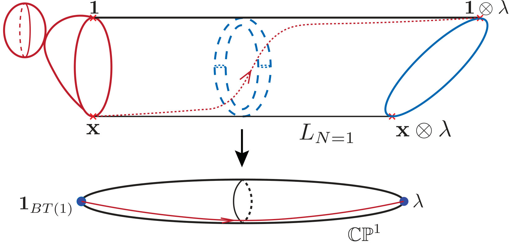 Figure 1
 Figure 2
 Figure 3
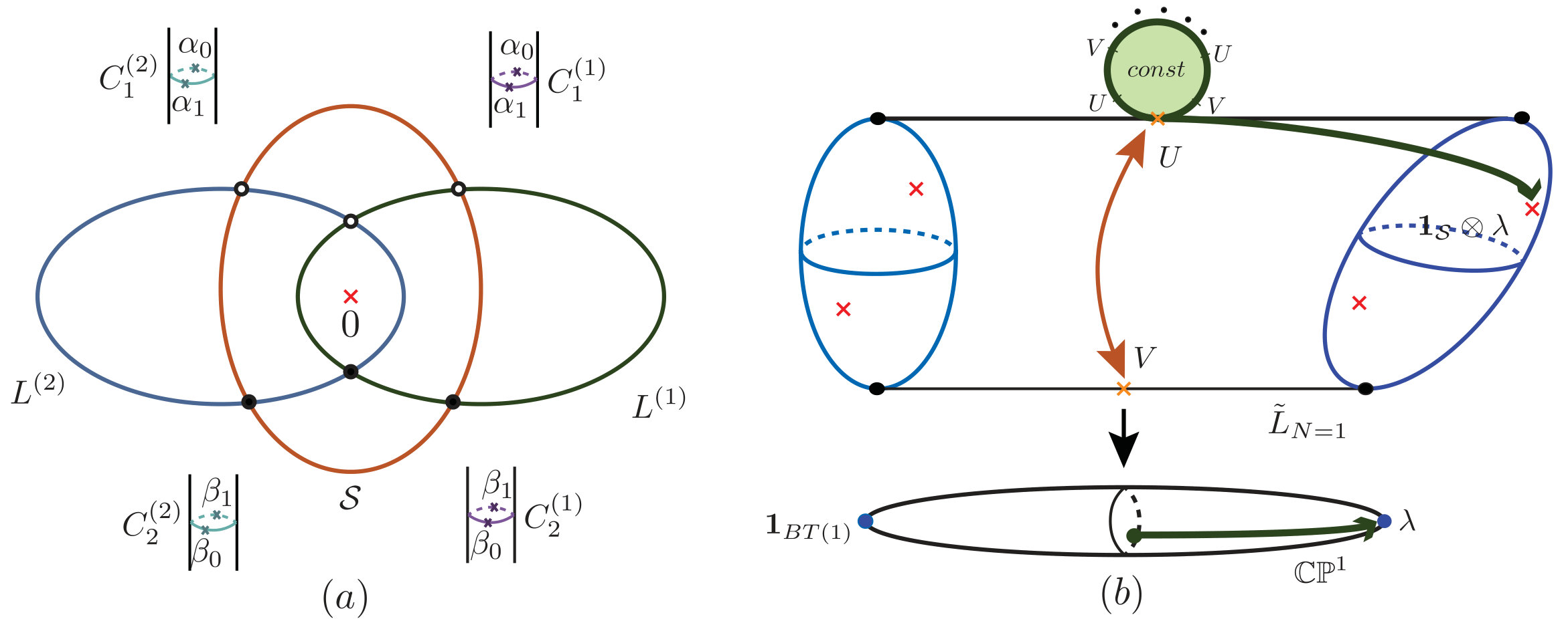 Figure 4
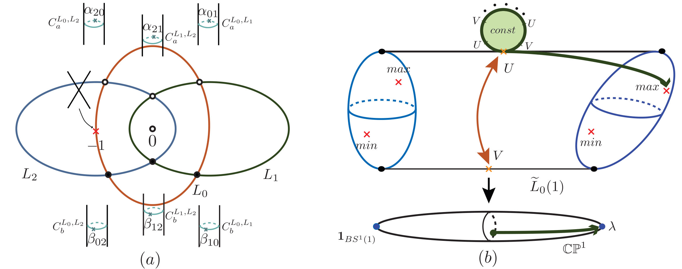 Figure 5
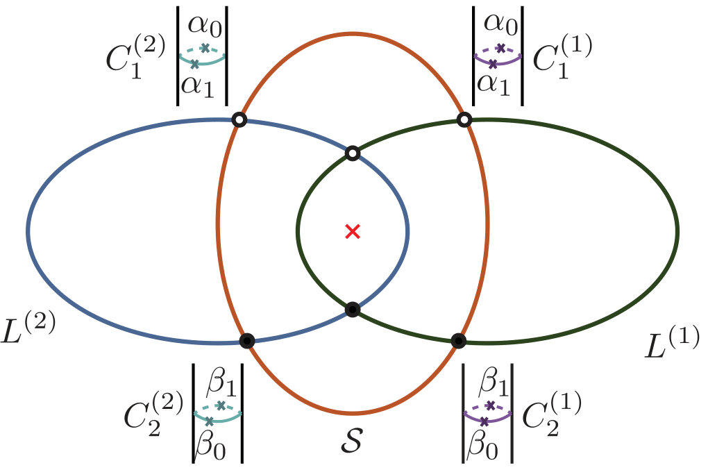 Figure 6
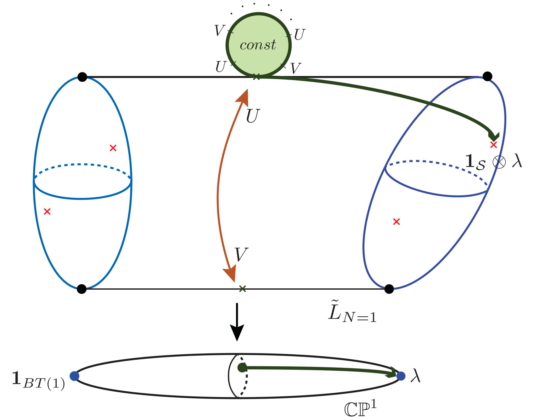 Figure 7
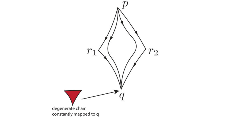 Figure 8
 Figure 9
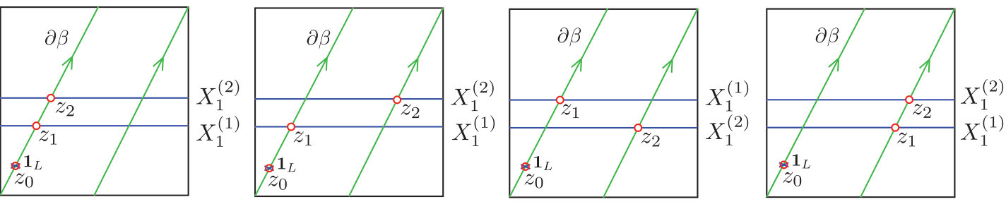 Figure 10
 Figure 11
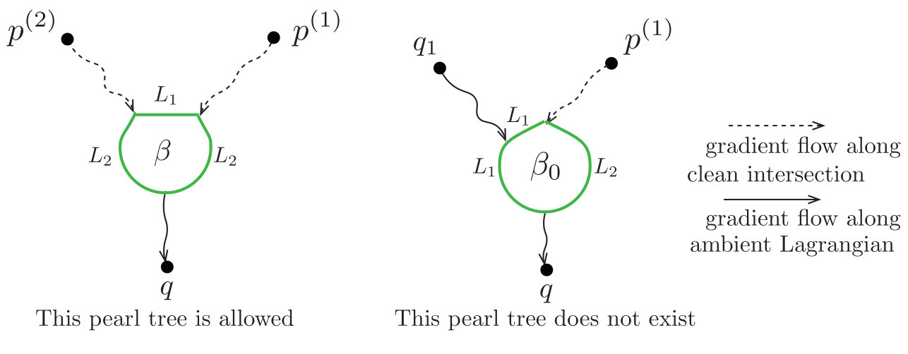 Figure 12
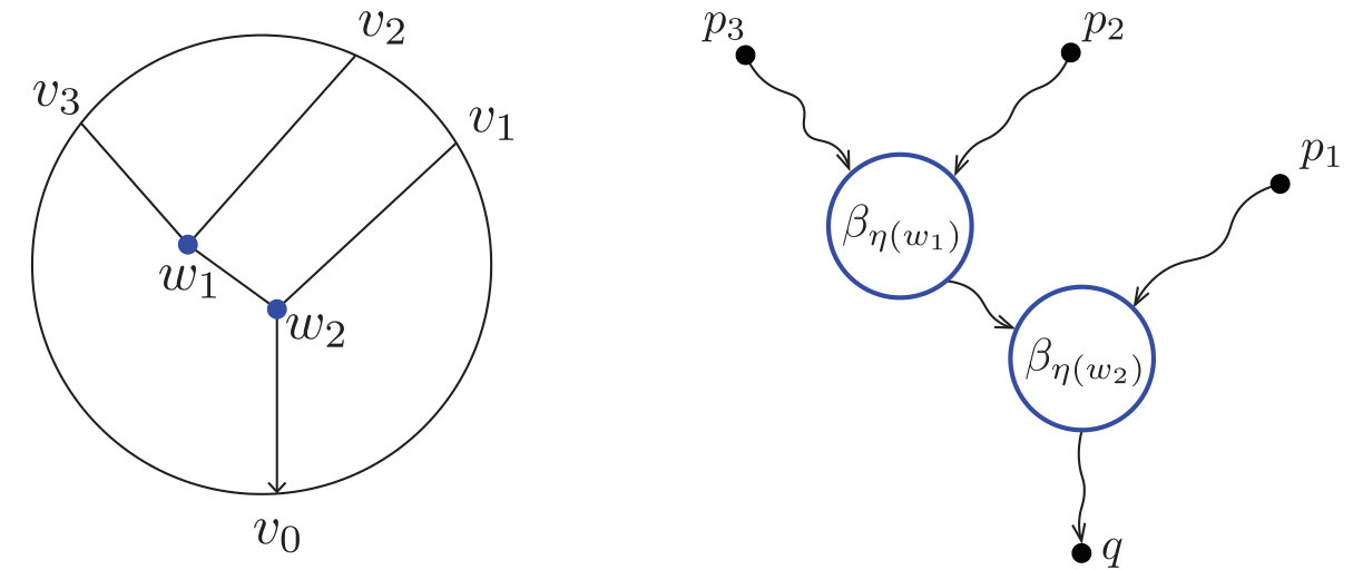 Figure 13
 Figure 14
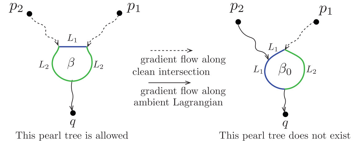 Figure 15
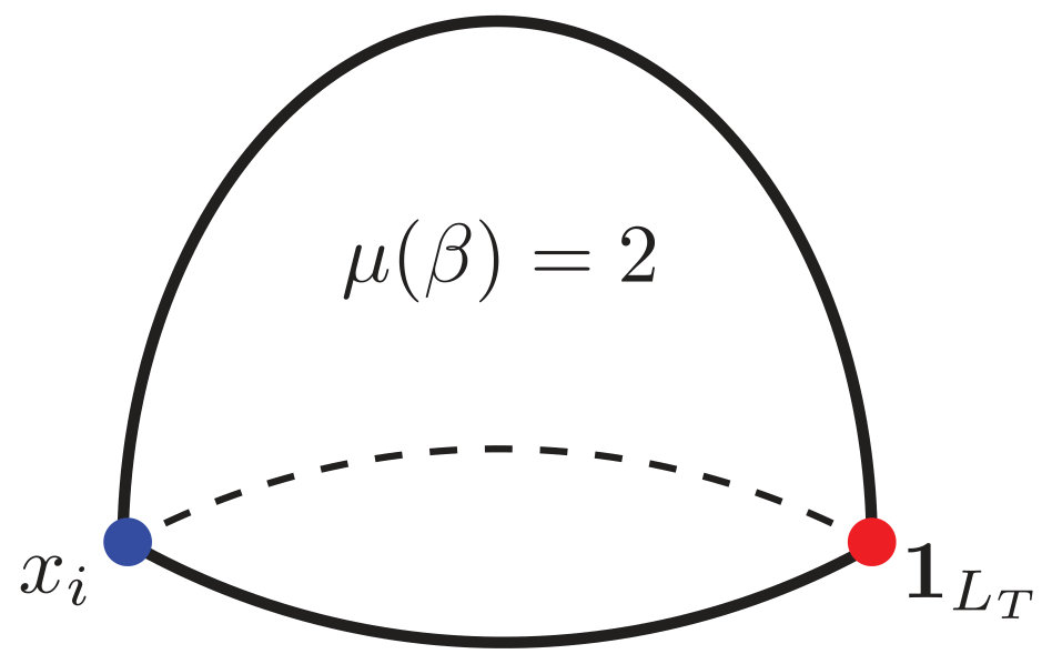 Figure 16
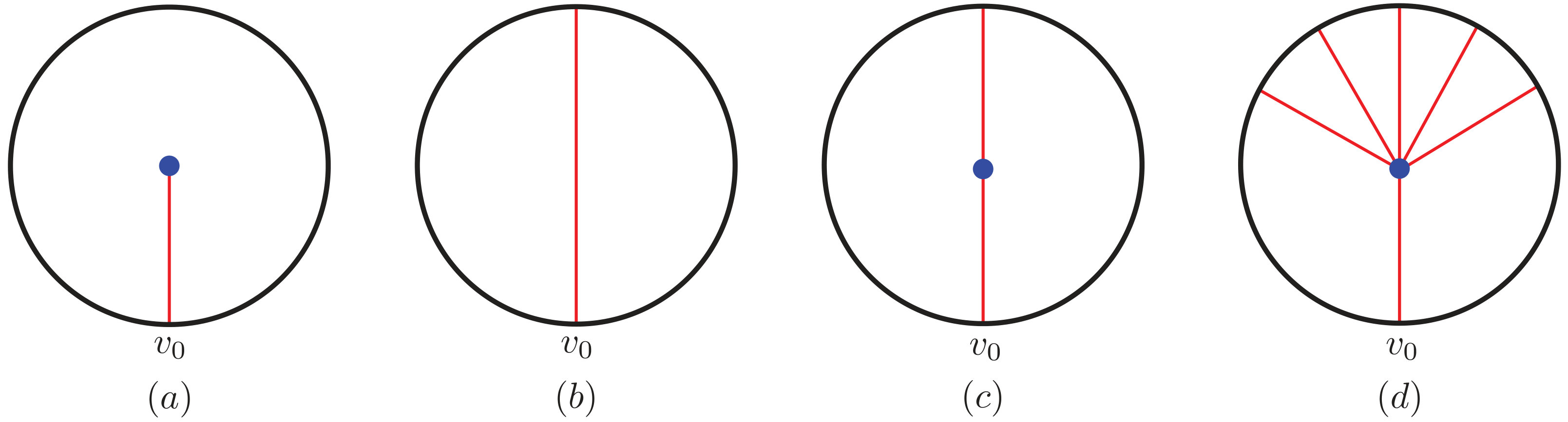 Figure 17
 Figure 18
Peer Reviews
No public reviews on file for this paper yet. If you reviewed it on a platform where reviews are public (OpenReview, ICLR, NeurIPS, ICML), you can paste yours below so the community can read it here.
Videos
No videos yet. Explain this paper in a talk, walkthrough, or lecture? Add one.
-equivariant disc potential and SYZ mirror construction
Yoosik Kim
Department of Mathematics, Brandeis University, 415 South Street Waltham, MA 02453, USA & Center of Mathematical Sciences and Applications, Harvard University, 20 Garden Street, Cambridge, MA 02138, USA
[email protected], [email protected]
,
Siu-Cheong Lau
Department of Mathematics and Statistics, Boston University, 111 Cummington Mall, Boston MA 02215, USA
and
Xiao Zheng
Department of Mathematics and Statistics, Boston University, 111 Cummington Mall, Boston MA 02215, USA
Abstract.
We develop a -equivariant Lagrangian Floer theory and obtain a curved algebra, and in particular a -equivariant disc potential. We construct a Morse model, which counts pearly trees in the Borel construction . When applied to a smooth moment map fiber of a semi-Fano toric manifold, our construction recovers the -equivariant toric Landau-Ginzburg mirror of Givental. We also study the -equivariant Floer theory of a typical singular SYZ fiber (i.e. a pinched torus) and compute its -equivariant disc potential via the gluing technique developed in [CHL18, HKL18].
Contents
- 1 Introduction
- 2 A Morse model for Lagrangian Floer theory
- 3 A Morse model for equivariant Lagrangian Floer theory
- 4 -equivariant disc potentials of toric manifolds
- 5 -equivariant disc potential for the immersed two-sphere
1. Introduction
Teleman [Tel14] conjectured that the mirror of a Hamiltonian action of a compact Lie group on a symplectic manifold is a holomorphic map from the mirror of to the space of conjugacy classes in . Moreover, the mirrors of the symplectic quotients for are closely related to the fibers this map. This agrees with the work of Hori-Vafa [HV00] on mirror symmetry via gauged linear sigma models.
An important step towards understanding this conjecture is to construct a such map. In this paper, we develop an equivariant version of the SYZ mirror construction using equivariant Lagrangian Floer theory. For a -inavariant Lagranguan submanifold of a Hamiltonian -manifold, its -equivariant disc potential gives a fibration of the mirror family over . For the concrete computations, we focus on the case when is a compact torus, and study the -equivariant Lagrangian Floer theory of torus fibers of an SYZ fibration.
For instance, let us consider the well-known Landau-Ginzburg mirror of a compact Fano toric -fold [HV00, Giv95, Giv98, LLY99]. It is given by a pair , where the superpotential is a holomorphic function of the form
[TABLE]
where are primitive generators of the one-dimensional cones of the fan defining , denote the corresponding Laurent monomials, and are Kähler parameters associated to effective curves classes .
Givental [Giv98] showed that the equivariant quantum cohomology of is mirror to the equivariant superpotential
[TABLE]
where are the equivariant parameters for the torus acting on . Iritani [Iri17b, Iri17a] further generalized this to a mirror correspondence between big equivariant quantum cohomology and a universal Landau-Ginzburg potential which has both equivariant and bulk-deformation parameters.
Cho-Oh [CO06] (in the Fano case) and Fukaya-Oh-Ohta-Ono [FOOO10] (in the general compact non-Fano setting) used Lagrangian Floer theory to define the disc potential of a smooth fiber of the toric moment map and showed that it coincides with the Landau-Ginzburg superpotential . From this perspective, is viewed as the generating function of open Gromov-Witten invariants. Each term in corresponds to a holomorphic disc of Maslov index bounded by the torus fiber. This gives an SYZ interpretation of the Landau-Ginzburg mirrors [Aur07, CL10].
It is a natural and interesting question that whether the can also be interpreted as a generating function of equivariant disc counts, to which we give an affirmative answer to in this paper.
Theorem 1.1** (Corolloary 4.10).**
Let be a semi-projective and semi-Fano toric manifold with , and let be the subtorus determined by the integral basis . The -equivariant disc potential (Definition 3.11) of a regular fiber of the toric moment map is given by
[TABLE]
where are the basic disc classes bounded by the toric fiber, is given by the inverse mirror map in equation (4.6), are the Kähler parameters, and is the formal Novikov variable.
In the Fano case, we have . By taking and to be the standard basis of , and setting for , the above expression for equals to .
In relation with the Teleman’s conjecture, the -equivariant disc potential for a Lagrangian submanifold with nonnegative minimal Maslov index takes the form
[TABLE]
for degree one weak bounding cochains . can be interpreted as follows: The equivariant term
[TABLE]
defines a map from the formal deformation space of to , assuming its convergence over . The non-equivariant term can be viewed as a family of potentials on the fibers of . It gives a mirror family of the symplectic quotient .
For instance, let us take . The non-equivariant part is simply . Suppose is a semi-Fano toric manifold. A fiber of is given by for some constants and . Then, the restriction of to the fibers give a mirror family of .
Remark 1.2**.**
The terms can be understood as obstruction terms for a homotopy equivalence between the equivariant Floer theory of and Floer theory of the quotient . Daemi-Fukaya [DF17] asserted that this homotopy equivalence can be constructed by Lagrangian correspondence. In our setting, we can compute the mirror equations explicitly.
The mirror map is crucial to precisely identify which fiber in the mirror family corresponds to . By the beautiful work of Woodward-Xu [WX18], the mirror map can be understood as the change from the gauged Floer theory of to the Fukaya category downstairs. Gauged Floer theory is formulated in terms of vortex equations. It would be very interesting to investigate the relation with our formulation.
Equivariant Lagrangian Floer theory has seen substantial recent developments. In the exact setting and , Seidel-Smith [SS10] provided an approach to understanding -equivariant Floer theory by combining Lagrangian Floer theory and family Morse theory [Hut08] on . Viterbo [Vit99] illustrated some related ideas for . Hendricks-Lipshitz-Sarkar [HLS16a, HLS16b] developed a homotopy coherent method to build up a -equivariant Floer theory. Daemi-Fukaya [DF17] used G-equivariant Kuranishi structure [Fuk17] to tackle the G-equivariant transversality problem, and make a formulation using differential forms. Bao-Honda [BH18] defined equivariant Lagrangian Floer cohomology for finite group action via semi-global Kuranishi structures. Mirror Lagrangian objects of equivariant vector bundles was studied by Lekili-Pascaleff [LP16]. There are many interesting works related to this subject such as [Sei].
In Section 3, we construct a Morse model for -equivariant Lagrangian Floer theory by counting pearly trees [BC07, FOOO09a] in the Borel construction , and study the associated equivariant disc potential. The key ingredient is a collection of Morse models on the finite dimensional approximations of satisfying certain compatibility conditions (Proposition 3.6). This is closest to the approach of Seidel-Smith, although the Lagrangians under our consideration are not exact. The Lagrangians of interest in this paper bound non-constant pseudo-holomorphic discs of non-negative Maslov index. These are known as quantum corrections in mirror symmetry, which can have non-trivial contributions to the equivariant parameters in the disc potential. Since there are only finitely many generators for each finite dimensional approximation of , it better serves for computations and for the SYZ mirror construction.
In order for the equivariant paramaeters appearing in to manifest. In Section 3.2 we adapt the homotopy unit construction developed by Fukaya-Oh-Ohta-Ono [FOOO09b, Chapter 7] to construct a curved -algebra
[TABLE]
which satisfies (Theorem 3.7)
[TABLE]
under the assumption that has minimal Maslov index zero and is a product of unitary groups. Here is the Novikov ring
[TABLE]
This allows us to view as a graded coefficient ring. We note that the terms of the form are series in the equivariant parameters and receive non-trivial contributions from pearly trees in .
In Section 5, we study the -equivariant Floer theory of the immersed two-sphere with a single nodal point. This is also known as the pinched two-torus and is the most common singular fiber appearing in an SYZ fibration. Even although it does not bound any non-constant holomorphic discs of Maslov index zero, it still has a non-trivial equivariant disc potential from the contribution of constant polygons at the nodal point. As the corresponding moduli spaces have non-trivial obstructions, the gluing technique via the isomorphism in the Fukaya category between smooth and pinched tori in [HKL18] is crucial in the computation of the explicit expression of the equivariant disc potential.
Theorem 1.3** (Theorem 5.7).**
The -equivariant disc potential of the immersed sphere is
[TABLE]
where , are the formal deformation parameters corresponding to the degree one immersed generators of .
Floer theory for immersed Lagrangians was developed by Akaho-Joyce [AJ10], which is in line with the theory of Fukaya-Oh-Ohta-Ono [FOOO09b] for smooth Lagrangians. In [DRET18], a different method via Legendrian topology is used to develop the Floer theory of immersed Lagrangian surfaces.
In a subsequent work [HKLZ19], we compute the equivariant disc potential for Lagrangian immersions in toric Calabi-Yau manifolds. They have very interesting expressions in relation with the Gross-Siebert slab functions [GS11] and mirror maps of toric Calabi-Yau manifolds [CLL12, CCLT]. It is closely related to the topological vertex [KL01, GZ02, FL13, FLT, FLZ16].
Acknowledgments
The first and second named authors express their deep gratitude to Cheol-Hyun Cho for explaining his point of view of equivariant Floer theory using Cartan model. The second named author also thanks Ben Webster and Kevin Costello for the discussion on Teleman’s conjecture at Perimeter Institute.
2. A Morse model for Lagrangian Floer theory
2.1. The singular chain model
Let be a symplectic manifold of real dimension . We assume that is convex at infinity or geometrically bounded if it is non-compact. Choose a compatible almost complex structure . For a closed, connected, and relatively spin Lagrangian submanifold , Fukaya-Oh-Ohta-Ono constructed a countably generated subcomplex of the singular chain complex (regarded as a cochain complex) and an -algebra . We briefly recall their construction below, which will be used in constructing the equivariant Morse model in Section 3. We refer the reader to [FOOO09b] for more details.
For , we denote by the moduli space of -holomorphic stable maps from a bordered Riemann surface of genus [math] representing and by the moduli space with boundary marked points ordered counter-clockwise. The moduli space has virtual dimension , where is the Maslov index of . It carries the evaluation map
[TABLE]
Let denote the monoid of effective classes in , represented by -holomorphic maps, i.e.
[TABLE]
For a -tuple of smooth singular chains of , we denote by the fiber product (in the sense of Kuranishi structures) of with , i.e.,
[TABLE]
We recall a generation , which will be used to determine perturbations of moduli spaces and subsets of singular chains inductively in [FOOO09b, Section 7]. As preliminaries, for , we first set
[TABLE]
where is the constant disc class. Also, we employ a function to keep track of generations of inputs. For a pair with , we define
[TABLE]
For a generation , we shall inductively choose a countable set of smooth singular chains on and a system of multisections for satisfying . Here the superscript is written to emphasize the generations of the inputs . Namely, at each inductive step, new multisections are chosen to be transversal to the zero section and extend the multisections previously chosen for the boundary strata . (To achieve transversality, the Kuranishi structures for the moduli spaces are chosen to be weakly submersive.) Moreover the zero locus
[TABLE]
is triangulated extending the triangulation on its boundary strata. The new simplices in the triangulation are then regarded as elements of . Additional singular simplices are added to so that
[TABLE]
remains a subcomplex of isomorphic on cohomology.
Let . The -map is defined by
[TABLE]
where
[TABLE]
Here, is the coboundary map on . The map is of degree .
Remark 2.1**.**
We note that it is only possible to choose finitely many multisections at once while still having them being sufficiently close to the original Kuranishi maps. To deal with this technical difficulty, Fukaya-Oh-Ohta-Ono introduced the notion of -structure associated to using moduli space of pseudo-holomorphic discs with bounded energy and number of marked points in [FOOO09b, Chapter 7]. The -structure on is obtained from the -structures via homological techniques.
Remark 2.2**.**
In order to define a -graded Floer cohomology, the conventional grading of the map is . This means aside from the case of graded Lagrangian submanifolds, one has to define the Novikov ring using an extra grading parameter in order to compensate for the Maslov indices. In this paper, we work on the chain level and do not follow this convention. The grading of is crucial in understanding the vanishing of certain terms when doing computations with the Morse model.
The singular chain model constructed in [FOOO09b] does not have a strict unit in general. It was shown that the fundamental cycle of is a homotopy unit. We briefly describe key properties and ideas below, and refer the readers to [FOOO09b, Chapter 3.3] for the precise definition of a homotopy unit and to [FOOO09b, Chapter 7.3] for details of the homotopy unit construction.
The constructed -algebra will be enlarged to a unital -algebra that is homotopy equivalent to . At first, we enlarge the chain complex by adding a generator of degree [math] serving as the strict unit and a generator of degree serving as a homotopy between and , that is,
[TABLE]
Then the -maps are defined with the following properties
- (1)
The restriction of to agrees with , 2. (2)
is the strict unit, i.e.
- (i)
for , 2. (ii)
for . 3. (3)
is a homotopy between and .
Later on, we will define a disc potential (Definition 2.8), which is to be of the most interest to us in the manuscript, after passing to the enlarged -algebra with a strict unit. To compute such a disc potential from the original singular chain model (before the enlargement), we need to examine the homotopy between and .
A construction and properties of the homotopy are in order. Let be an ordered subset of satisfying . For with , let be the -tuple obtained by inserting into the -th places of . We assume . We set if where . Consider the forgetful map
[TABLE]
which forgets the -th marked points and then stabilizes.
We choose a perturbation on as follows: For a splitting of , we denote by the -tuple given by removing from the -th places of . Let be coordinates on . If for all , we take the perturbation transversal to the zero section obtained by just inserting into the -th place. If for all , we take the perturbation pulled back via the map in (2.3). Finally, we take a perturbation on transversal to the zero section interpolating between them.
The maps for with inputs inserted into -th place of are defined by
[TABLE]
where is the equivalence relation collapsing fibers of , see [FOOO09b, Definition 7.3.28]. Notice that the zero locus of a pullback multisection is a degenerate singular chain which becomes zero in the quotient.
We also set and therefore
[TABLE]
where
[TABLE]
Note that and the terms
[TABLE]
are of degrees at most and therefore are degenerate singular chains.
2.2. Morse homology singular homology: an alternative approach
Pearl complex was developed by Biran and Cornea [BC07, BC09] for monotone Lagrangians (a similar complex also appeared in an earlier work of Oh [Oh96]). It has many important applications, including the proof of homological mirror symmetry for Fermat Calabi-Yau hypersurfaces by Sheridan [She15].
A Morse model of Lagrangian Floer theory was constructed in [FOOO09a] based on their singular chain model. We follow their construction to construct a Morse model in Section 2.3, with a modification that we add certain degenerate chains as summands in the definition of unstable chains of critical points and the chains of forward orbits of singular chains . The main reason for the modification is that there are unwanted degenerate chains appeared in and , and we ‘contract them away’ by adding the cones over the unwanted terms. This modification enables us to realize a Morse complex as a singular chain complex, which will be explained in this section.
Let be a Morse function. Let be a negative pseudo-gradient vector field for , i.e. and the equality holds if and only if . For each , coincides with the negative gradient vector field for the Euclidean metric on a Morse chart of . Let be the flow of . For each , we denote by and its stable and unstable manifolds respectively. Namely,
[TABLE]
The degree of is denoted by and defined by
[TABLE]
where is the Morse index of . Then . Let be the cochain complex
[TABLE]
with grading given by .
We assume that satisfies the Smale condition and call such a pair Morse-Smale. For , let be the moduli space of flow lines from to . The Smale condition implies
[TABLE]
The moduli space and the unstable manifold have natural compactifications to smooth manifolds with corners and whose codimensional strata consist of -times broken flow lines
[TABLE]
and
[TABLE]
In particular, we have
[TABLE]
In [FOOO09a], a (non-unital) -algebra structure was constructed on assuming has a triangulation whose simplices are the closures of . To establish an isomorphism between Morse and singular cohomology, we have to associate to each critical point of degree a singular chain . A natural candidate for is a fundamental chain for . If we make such a natural choice, several issues occur.
Suppose that we choose such a natrual chain . From (2.7), one can see that in general has boundary components of the form with . Since , and the image of in is supported on , the facet of representing is a degenerate chain on . Thus, for the assignment to be a chain map, one should deal with degenerate chains. On the other hand, are constructed including degenerate chains since the product of degenerate chains may no longer be a degenerate chain.
We overcome this difficulty by adding certain degenerate chains to the fundamental chains (of the compactified unstable submanifolds) and define a map by accordingly such that it is a chain map which induces an isomorphism on cohomology, see Figure 1.
More details of a modification are in order. We start with smooth cubical singular chains
[TABLE]
representing the fundamental classes of and , respectively. Their boundaries are given as
[TABLE]
To regard as simplicial singular chains, we choose triangulations for (the domain of) and inductively on . For any critical point with , and are [math]-simplices. Suppose that we have chosen triangulations for and for any with . For , with are [math]-simplices. Suppose we have chosen triangulation for for , . For , we first triangulate as follows: each in is a product of simplicial complexes. We choose linear orders on vertices of and (compatible with their orientations). Then there exists a unique triangulation of such that the vertices of are pairs , where is a vertex of and is a vertex of , and an -simplex in is defined by a set such that , , defines a simplex on and defines a simplex on with . Notice that this is the standard product structure in the category of simplicial sets. We then triangulate extending the triangulation on . Finally, we triangulate extending the triangulation on given by .
For each in the boundary of , let be the (simplicial) cone over with vertices
[TABLE]
and simplices
[TABLE]
for . In particular, this means is the vertex of the cone. As a singular chain on , the map is defined by composing the contraction with the map . Note that for two simplicial complexes and , we have .
We construct inductively on as follows: For , we set . Suppose we have constructed for . For , we define
[TABLE]
and set
[TABLE]
By construction, we have
[TABLE]
Theorem 2.3**.**
We define a map
[TABLE]
where is as defined in (2.8). Then the map is a chain map which induces an isomorphism on cohomology where denotes the Morse differential.
Remark 2.4**.**
The approach in [HL99] is to mod out by degenerate chains. If we were to consider modded out by the subcomplex of degenerate chains, a proof can be found therein. Since we do not wish to mod out by degenerate chains, we would have to modify their arguments.
Before proving Theorem 2.3, let us introduce some terminologies. We say a smooth singular chain is generic if each face of every simplex intersects the stable submanifolds of the critical points of transversely. Let be the subcomplex of generated by the generic singular chains. It is easy to see that and are isomorphic on cohomology.
For a generic simplex , we denote by the moduli space of flow lines from to a critical point . Its dimension is given by . Let denote the codimension strata of . The moduli space has a natural compactification to a smooth manifold with corners . Its strata of codimension are
[TABLE]
For , we have
[TABLE]
We define the forward orbit of to be the set with the map
[TABLE]
where is the flow of the negative pseudo-gradient vector field . The orbit has a natural compactification to a smooth manifold with corners , whose codimension strata are
[TABLE]
When , we have
[TABLE]
Now, we are ready to prove the main theorem of this section.
Proof of Theorem 2.3.
The assertion that is a chain map follows from (2.9). To show that induces an isomorphism on cohomology, we modify the proof in [HL99]. We have a chain map defined by
[TABLE]
In particular, is empty when is a degenerate simplex. Clearly, .
We define a homotopy as follows. Let be a smooth cubical singular chain in representing the fundamental class of satisfying
[TABLE]
We again triangulate inductively on the dimension to regard them as simplicial singular chains. We also choose smooth singular chains representing the fundamental class of satisfying
[TABLE]
We then construct inductively on by first replacing with on and then gluing to the boundary of the resulting chain. This ensures that is a chain homotopy between and the identity, i.e., satisfies
[TABLE]
as desired. ∎
2.3. Morse model with a strict unit
In this section, by adapting the homotopy unit construction in [FOOO09b, Chapter 7] (see also Charest-Woodward [CW15]) and using Theorem 2.3, we will explain how to construct a unital -algebra on a pearl complex.
For simplicity, we will always assume has a unique maximum point , so that is the fundamental cycle. Let
[TABLE]
with and |\bm{1}^{{\color[rgb]{.5,.5,.5}\definecolor[named]{pgfstrokecolor}{rgb}{.5,.5,.5}\pgfsys@color@gray@stroke{.5}\pgfsys@color@gray@fill{.5}\blacktriangledown}}|=-1. The superscripts , and {\color[rgb]{.5,.5,.5}\definecolor[named]{pgfstrokecolor}{rgb}{.5,.5,.5}\pgfsys@color@gray@stroke{.5}\pgfsys@color@gray@fill{.5}\blacktriangledown} are borrowed from [CW15]. We extend the Morse differential to by setting
[TABLE]
We now construct a unital -algebra structure on . Let
[TABLE]
For , suppose had been constructed for all generations . The perturbations and in (2.1) and (2.4) can be chosen to have the following properties: Let be any face of either a simplex in the triangulation of
[TABLE]
or a simplex in the triangulation of
[TABLE]
- (1)
is transversal to the stable submanifold for all 2. (2)
For each of dimension at most , there exists at most one critical point such that is of complementary dimension to and intersects at a unique point.
Denote by the set of those singular simplices . Define where is given by
[TABLE]
if there exists a unique such that intersects at a unique point, and , otherwise. In particular, we have whenever is a degenerate simplex.
We further add the simplices (defined in the proof of Theorem 2.3) for every to . For chains of the form , we put . The maps and obey
[TABLE]
for .
Set
[TABLE]
We recall that is the unit and is a homotopy between and the fundamental class . We extend the coboundary operator to by setting
[TABLE]
We then extend and to maps and respectively by setting
[TABLE]
so that (2.12) holds for any .
A homological perturbation can be applied to reduce the -algebra structure on in (2.2) to that on in (2.13). We identify the latter with via the map defined by (2.10) and the following assigments
[TABLE]
The resulting unital -algebra is denoted by . By following [FOOO09a, Theorem 5.1], we obtain
Theorem 2.5**.**
The Morse model is a unital -algebra. Moreover, the Morse model and the singular model in (2.2) are unital homotopy equivalent.
We explicitly describe the -structure maps of the Morse model . The maps are given in terms of maps and associated to decorated planar rooted trees. Let us fix a labeling of elements of where is the constant disc class.
Definition 2.6** ([FOOO09a]).**
A decorated planar rooted tree is a quintuple consisting of
- •
is a tree;
- •
is an embedding into the unit disc;
- •
is the root vertex and ;
- •
is the set of interior vertices with valency ;
- •
.
where is the set of vertices; is the set of exterior vertices and is the set of interior vertices. For , denote by the set of isotopy classes represented by with and if the valency of is or . In other words, the elements of are stable.
We denote by the unique tree with no interior vertices. For this tree , set
[TABLE]
where is the inclusion map in (2.14). For each , contains a unique element that has a single interior vertex , which is denoted by . We then define
[TABLE]
For general , we cut it at the vertex closest to so that is decomposed into and an interval adjacent to in the counter-clockwise order. We inductively define
[TABLE]
Finally, we define the -map by
[TABLE]
where .
The maps restricted to are given by counting pearly trees as depicted in Figure 2 (This observation was made in [FOOO09a]. See also [CW15] for a description of with general inputs in terms of pearly trees). For a decorated tree , the exterior vertices are labeled respecting the counter-clockwise orientation. Each edge is oriented in the direction from the input vertices to the root vertex . We denote by the edge attached to and by the vertices such that is the edge from to . For , consider the moduli space consisting of the following configurations:
- •
for each interior vertex , a bordered stable map representing the class with boundary marked points. We denote by the marked point corresponding to the edge attached to ;
- •
for , the input edge corresponds to a flow line from to ;
- •
the output edge corresponds to a flow line from to ;
- •
an interior edge corresponds to a flow line from to .
The virtual dimension of is given by
[TABLE]
where . The map is given by
[TABLE]
where is the signed count of the moduli space of virtual dimension [math].
2.4. Disc potentials in Lagrangian Floer theory
In this section, we recall the disc potential of introduced by Fukaya-Oh-Ohta-Ono [FOOO09b].
We denote by the maximal ideal
[TABLE]
Let be an -algebra over with the strict unit , and set
[TABLE]
The weak Maurer-Cartan equation for an element is given by
[TABLE]
The condition that ensures the convergence of . A solution of (2.4) is called a weak bounding cochain. We denote by
[TABLE]
the space of weak Maurer-Cartan elements. We say an -algebra is weakly unobstructed if is nonempty, in which case we have for any , thus defining a cohomology theory .
Let us put
[TABLE]
For an element , we can define a deformation of the -structure by
[TABLE]
Now, for , we denote by the space of odd degree weak bounding cochains. In general, one should also consider gauge equivalences between weak Maurer Cartan solutions. However, we omit them here since they will trivial in our examples.
We say that the deformation of by (or simply ) is unobstructed (resp. weakly unobstructed), if (resp. ). In particular, if , we will simply say is unobstructed.
The following lemma concerns the weakly unobstructedness of . This technique of finding weak bounding cochains in the presence of a homotopy unit was introduced in [FOOO09b, Chapter 7] and [CW15, Lemma 2.44].
Lemma 2.7**.**
Let . Suppose and the minimal Maslov index of is nonnegative. Then there exists such that , i.e., is weakly unobstructed. In particular, if the minimal Maslov index of is at least two, then, .
Proof.
By (2.5), we have
[TABLE]
where
[TABLE]
is a multiple of . The vanishing of the contribution of higher Maslov index discs follows from the fact that the output singular chains are of degrees at most , whose projection to vanishes. Hence we can write (2.17) as
[TABLE]
for some .
Let us tentatively take b^{\prime}=b+\bm{1}^{{\color[rgb]{.5,.5,.5}\definecolor[named]{pgfstrokecolor}{rgb}{.5,.5,.5}\pgfsys@color@gray@stroke{.5}\pgfsys@color@gray@fill{.5}\blacktriangledown}}. We have
[TABLE]
The second equality is due to the vanishing of the maps with more than one \bm{1}^{{\color[rgb]{.5,.5,.5}\definecolor[named]{pgfstrokecolor}{rgb}{.5,.5,.5}\pgfsys@color@gray@stroke{.5}\pgfsys@color@gray@fill{.5}\blacktriangledown}} as an input since the outputs are of degrees at most . Also, notice that the terms \mathfrak{m}_{1,\beta}^{b}(\bm{1}^{{\color[rgb]{.5,.5,.5}\definecolor[named]{pgfstrokecolor}{rgb}{.5,.5,.5}\pgfsys@color@gray@stroke{.5}\pgfsys@color@gray@fill{.5}\blacktriangledown}}) are of degree [math] and therefore are multiples of .
Using the notation of (2.18), we can write
[TABLE]
Since there do not exist any gradient flow lines from to the maximum , the contribution of the terms
[TABLE]
are zero and hence .
Now, set b^{+}=b+\frac{W}{1-h(b)}\bm{1}^{{\color[rgb]{.5,.5,.5}\definecolor[named]{pgfstrokecolor}{rgb}{.5,.5,.5}\pgfsys@color@gray@stroke{.5}\pgfsys@color@gray@fill{.5}\blacktriangledown}}. We have
[TABLE]
which yields .
If the minimal Maslov index of is at least two, then (see (2.6)) and hence . ∎
Let the space of elements which satisfy
[TABLE]
By the above lemma, for each such , there exists such that . Then, can be viewed as a function on .
Definition 2.8**.**
We will call the disc potential of .
3. A Morse model for equivariant Lagrangian Floer theory
There are several approaches to -equivariant Lagrangian Floer theory for a pair of G-invariant Lagrangians in the existing literature. For , Seidel-Smith [SS10] used Floer homology coupled with Morse theory on to define -equivariant Lagrangian Floer homology of exact Lagrangians. In [HLS16a, HLS16b], Hendricks-Lipshitz-Sarkar used a homotopy theoretic method to define -equivariant Lagrangian Floer homology for a compact Lie group . Daemi-Fukaya [DF17] defined an equivariant de Rham model using -equivariant Kuranishi structures developed in [FOOO09b, Fuk17]. Bao-Honda [BH18] defined equivariant Lagrangian Floer cohomology in the case of finite group action via semi-global Kuranishi structures.
In this section, we develop a Morse model for the -equivariant Lagrangian Floer theory focusing on a single -invariant Lagrangian. The underlying cochain complexes can be constructed such that each complex is finite dimensional over the cohomology ring of , and the -maps are given by counting pearly trees in the Borel construction . This suits better for our purpose of computing disc potentials and constructing SYZ mirrors. The -algebra we construct will be unital. This uses the homotopy unit construction in [FOOO09b], which has also been adapted to the stabilizing divisor perturbation scheme by Charest-Woodward [CW15] for their (non-equivaraint) unital Morse model.
We define the -equivariant Lagrangian Floer theory as the (ordinary) Lagrangian Floer theory of as a Lagrangian submanifold of a certain symplectic manifold . This avoids the issue of equivariant transversality. The Morse model we use makes the theory much more explicit and computable. Since the Lagrangians we study here bounds non-constant pseudo-holomorphic discs, we use the machinery of [FOOO09b] to handle the obstructions. On the other hand, for computing the equivariant disc potential of toric Fano manifolds, virtual technique is not necessary.
3.1. The equivariant Morse model
Let be a compact Lie group. We begin by choosing smooth finite dimensional approximations for the universal bundle over the classifying space. Namely, we have the follwing diagram
[TABLE]
where and are compact smooth manifolds, and the horizontal arrows are smooth embeddings. We note that are connected for since is -connected.
We also consider the cotangent bundles and equipped with the canonical symplectic forms. Every symplectic -action on a symplectic manifold can be naturally lifted to a Hamiltonian -action on its cotangent bundle. We choose a moment map for the Hamiltonian -action on lifted from the -action on where is the dual Lie algebra of . Since acts on freely, we have a canonical isomorphism
[TABLE]
as symplectic manifolds. We denote by the almost complex structure induced by a -invariant compatible almost complex structure on . Notice that is compatible with the canonical symplectic form on .
Let be a symplectic -manifold, i.e. is a symplectic manifold endowed with a -action which preserves . As in Section 2.1, is assumed to be convex at infinity or geometrically bounded if it is non-compact. Let be a -invariant, closed, connected, and relatively spin Lagrangian submanifold . We will assume the relative spin structure is preserved by the -action. Let us fix a -invariant almost complex structure compatible with . In this section, we will define a Morse model for the -equivariant Lagrangian Floer theory on .
Let and set . Since acts freely on , there is a canonical map , which is a fiber bundle with the fiber . Let be inclusion of a fiber. By the construction, is endowed with a symplectic form and a compatible almost complex structure satisfying
[TABLE]
and
[TABLE]
Let for , which are finite dimensional approximations of the Borel construction . We note that is a fiber bundle with the fiber . Regarding as the zero section of , is a Lagrangian submanifold of for each . The diagram (3.1) induces a commutative diagram
[TABLE]
where the vertical arrows are embeddings of Lagrangian submanifolds.
Now, we study the disc moduli bounded by . The following proposition tells us that the image of any stable -holomorphic map must be fully contained in a fiber of the map .
Proposition 3.1** (Effective disc classes).**
The induced map restricts to a bijection
[TABLE]
Proof.
Suppose that there is a -holomorphic map .
[TABLE]
Then the composition is a -holomorphic disc in bounded by the zero section . Since is an exact Lagrangian of , it does not bound any non-constant pseudo-holomorphic discs. It implies that is necessarily constant and is contained in a fiber of over . ∎
Proposition 3.1 has the following corollaries that will play an important role in computing the disc potential of later on.
Corollary 3.2** (Maslov index).**
The Maslov index of is equal to the Maslov index of .
By abuse of notation, we denote the disc classes and both by . We also denote their Maslov index by and symplectic area by .
Corollary 3.3** (Regularity).**
A -holomorphic disc is regular if it is regular as a disc in the corresponding fiber of .
Proof.
Let and . We denote by the space of smooth global sections of E with boundary values in and by the space of smooth global -forms with coefficient in . Consider the two term elliptic complex
[TABLE]
where is the linearized Cauchy-Riemann opeartor at . Pulling the following exact sequences
[TABLE]
and
[TABLE]
via , we choose splittings
[TABLE]
and
[TABLE]
where and are subbundles. This gives a decomposition of (3.3)
[TABLE]
By Proposition 3.1, is a constant map and hence is surjective. Therefore, is surjective if and only if is surjective. ∎
Our heuristic definition of a -equivariant Lagrangian Floer theory is the (ordinary) Lagrangian Floer theory of the Lagrangian submanifold . However, since is infinite dimensional, we resort to using finite dimensional approximations associated to a sequence of Morse-Smale pairs on . Clearly, arbitrary choices of and Kuranishi perturbations would not suffice for this purpose. We begin by specifying our choices of Morse-Smale pairs.
Definition 3.4**.**
We call a sequence of Morse-Smale pairs admissible if it satisfies the following:
- (1)
For each , there is an inclusion of critical point sets . Under this identification, we have
- (i)
For , . 2. (ii)
For , the image of in coincides with in . 3. (iii)
For , we have for all . This implies
[TABLE]
for . 2. (2)
For each , there exists an integer such that for all and . 3. (3)
The Morse function has a unique maximum and the inclusion identifies with . This allows us to identify with a subcomplex of . We will denote , and \bm{1}^{{\color[rgb]{.5,.5,.5}\definecolor[named]{pgfstrokecolor}{rgb}{.5,.5,.5}\pgfsys@color@gray@stroke{.5}\pgfsys@color@gray@fill{.5}\blacktriangledown}}_{L(N)} simply by , , and \bm{1}^{{\color[rgb]{.5,.5,.5}\definecolor[named]{pgfstrokecolor}{rgb}{.5,.5,.5}\pgfsys@color@gray@stroke{.5}\pgfsys@color@gray@fill{.5}\blacktriangledown}}.
We explain below how such a sequence of Morse-Smale pairs can be produced. This is inspired by the family Morse theory of Hutchings [Hut08].
Proposition 3.5**.**
A smooth model for can be chosen such that admissible sequences of Morse-Smale pairs exist.
Proof.
We choose to be the infinite Stiefel manifold and to be the infinite Grassmannian . We have an embedding of into the skew-Hermitian matrices on by identifying with the orthogonal projection onto . Let be the diagonal matrix with entries . The map
[TABLE]
is a perfect Morse function (see [Nic94]). We note that has the following properties:
- (1)
The restriction
[TABLE]
of to each finite dimensional stratum is again a perfect Morse function. 2. (2)
For all and , we have
[TABLE] 3. (3)
If a critical point of is contained in , then .
We fix an embedding of Lie groups for some , and choose and . This gives a fibration with fibers the homogeneous space . Let be an open cover such that each is contractible, and if and , then . Let be a partition of unity subordinate to . Notice that are constant near the critical points of due to our second assumption on the open cover.
Let be a Morse function and define by
[TABLE]
Here and are understood as defined on the local trivializations . For each , the restriction of to generic fibers of is a Morse function. In particular, the restriction of to each fiber over a critical point of agrees with .
We set
[TABLE]
Since is compact, for sufficiently small , has the critical point set
[TABLE]
Moreover, is a Morse function. The non-degeneracy of critical points follows from the fact that are constant near the critical points of .
Now, let be a negative pseudo-gradient vector field for such that is a Morse-Smale pair, and let be a fiberwise negative pseudo-gradient for . We set
[TABLE]
where denotes the horizontal lift with respect to an auxiliary connection for the fiber bundle . For each , we put . Then, for a generic choice of , the pairs are Morse-Smale.
Finally, let be a Morse function. By iterating the construction in the above paragraphs, we obtain Morse-Smale pairs with
[TABLE]
It follows from the properties of that is an admissible collection in the sense of Definition 3.4. ∎
We now turn to the choice of Kuranishi structures on the moduli spaces . Let us first recall that for an element , a Kuranishi chart around is a quintuple , where is the finite automorphism group of acting on the vector bundle , is a smooth manifold with corners parameterizing smooth stable maps close to , is a -equivariant smooth section of , and is a homeomorphism from to a neighborhood of .
We fix weakly submersive Kuranishi structures for the disc moduli following [FOOO09b, Chapter 7.1]. For , since the holomorphic discs with boundary on are contained in the fibers of (over ), there are no obstruction in the base direction, and therefore we can choose Kuranishi structures to be of the following form: For every and , we choose a contractible neighborhood of in and trivializations and compatible with the diagram (3.2). This gives an trivialization of . Then, for an element in a fiber of , we can take the (weakly submersive) Kuranishi chart around to be
[TABLE]
where is the pullback of via the projection Then we have
[TABLE]
as Kuranishi structures. Moreover, we can orient the moduli spaces using a -invariant relative spin structure such that the orientations are compatible with the restriction above.
Let be Morse models associated to an admissible collection of Morse-Smale pairs . Let be the map induced by inclusion of critical points . We denote by the -structure maps on the singular chain models and by the maps associated to the decorated planar rooted trees in the definition of .
The next key proposition enables us to define the -structure maps of -equivariant Lagrangian Floer theory.
Proposition 3.6**.**
The singular chain models can be constructed such that the resulting unital Morse models satisfy the following property:
[TABLE]
for and . Here, the (RHS) means that we only consider the outputs of in .
Proof.
We proceed by induction on . For , the statement of the proposition is void. Suppose we have constructed -algebras for all with satisfying (3.6). We now construct satisfying (3.6) as follows:
Let be the subset
[TABLE]
Inductively on , we construct the set of singular simplices , and choose perturbations , , and , with following additional properties
- (1)
There exists a bijection . 2. (2)
For , , and , we have
[TABLE]
as Kuranishi structures, where . 3. (3)
For , with , we have
[TABLE]
as Kuranishi structures, where . In particular, if , then . 4. (4)
Let for . Let be the perturbation chosen at the previous inductive step on for . If , then for each , there is a one-to-one correspondence between the following sets of simplices. The first set is the set of simplices in the triangulation of
[TABLE]
which are of complementary dimension to the stable submanifold in and intersect at a unique point. The other set is the set of simplices in the triangulation of
[TABLE]
which are of complementary dimension to the stable submanifold in and intersect at a unique point. Moreover, the intersection points for the corresponding simplices have the same orientation. 5. (5)
The analogue of (4) holds for the perturbation and the simplices in the triangulation of
[TABLE]
These properties together would imply that the resulting Morse model satisfies property (3.6).
Denote by the unstable chain of defined as in (2.8). For , we have
[TABLE]
by Definition 3.4 (1). We define by .
Let , . For , let , and let be the -tuple obtained by inserting into the -th places of . Since any holomorphic disc is contained in a fiber of over by Proposition 3.1, Definition 3.4 (1) implies
[TABLE]
and
[TABLE]
as compact subsets of and , respectively. The restriction of the natural Kuranishi structure for the fiber product (resp. ) to the (LHS) of (3.9) (resp. (3.10)) agrees with the Kuranishi structure of the (RHS) of (3.9) (resp. (3.10)). This establishes properties (1)-(3). Notice that properties (4), (5) are void for .
Now, suppose we have constructed singular simplices and chosen perturbations satisfying (1)-(5) for . Let for . Suppose . Then , and by inductive hypothesis on , we have
[TABLE]
as Kuranishi structures. We choose perturbation to extend the perturbation and the perturbation for the boundary strata . Note that is compatible with the perturbation for since the latter is extended from the perturbation for at previous inductive steps on .
We triangulate extending the triangulation on
and triangulation on the boundary strata. We can choose the perturbation such that any simplex in this triangulation away from is transverse to the stable submanifolds of (via the evaluation map ). Suppose is a simplex in this triangulation and . By subdividing if necessary, we can assume that has a face in and no other faces of of dimension greater or equal to are in . Notice that is not transverse to all stable submanifolds of since the stable submanifolds remain unchanged by Definition 3.4 (1) but the ambient space is of higher dimension than . We can however move the vertices of so that it is transverse to the stable submanifolds of . We choose the perturbation and the triangulation for in a similar manner.
Finally, we define by , and . ∎
We are now ready to define a Morse model for the -equivariant Lagrangian Floer theory of . The equivariant Floer complex is defined to be the direct limit
[TABLE]
In order to define the -structure maps on , we first define the maps for and as follows. For , there exists a sufficiently large such that . Setting , we define by
[TABLE]
where comes from Definition 3.4 (2). Because of Proposition 3.6, (3.12) is defined independent of the choice of . Finally, we define the maps by
[TABLE]
[TABLE]
The pair is an -algebra with a strict unit . For fixed inputs the -identity can be checked on for sufficiently large .
We will refer to the pair from (3.11) and (3.14) as the Morse model for the -equivariant Lagrangian Floer theory (-equivariant Morse model) of .
3.2. Equivariant parameters as homotopy partial units
Consider a Lagrangian toric fiber of a compact semi-Fano toric manifold of the complex dimension. One of the main goals of this paper is to understand the Givental’s equivariant toric superpotential
[TABLE]
as the disc potential of the -equivariant Lagrangian Floer theory of constructed in Section 3.1. The terms are the equivariant parameters generating the cohomology ring
[TABLE]
Since have cohomological degree , the expression (3.15) of suggests that the boundary deformations of curvature are, a priori, obstructed. For this reason, we shall construct in this section an alternative model which is homotopy equivalent to our equivariant Morse model and define its equivariant disc potential. Our construction in this section replies on the existence of a well-behaved perfect Morse function on (e.g. (3.4) for ). For this reason, we will temporarily restrict the discussion to the case when is a product of unitary groups.
To begin with, we fix a Morse function on with a unique maximum point . Following the proof of Proposition 3.5, we can choose an admissible sequence of Morse-Smale pairs such that is of the form
[TABLE]
where
- •
is a perfect Morse function on .
- •
is a (generically) fiberwise Morse function for . In particular the restriction of to each fiber over a critical point of agrees with for some .
Since the choice (3.16) satisfies (3.5), we have
[TABLE]
We then enlarge fiberwise over to
[TABLE]
where
[TABLE]
as in (2.11).
We shall produce a unital -algebra structure on
[TABLE]
over the graded coefficient ring via finite dimensional approximations. Set
[TABLE]
Here, the singular chains in are the unstable chains of the critical points of . We denote by the unstable chain of the critical point . The generators and \bm{\lambda}^{{\color[rgb]{.5,.5,.5}\definecolor[named]{pgfstrokecolor}{rgb}{.5,.5,.5}\pgfsys@color@gray@stroke{.5}\pgfsys@color@gray@fill{.5}\blacktriangledown}} are of degrees and |\bm{\lambda}^{{\color[rgb]{.5,.5,.5}\definecolor[named]{pgfstrokecolor}{rgb}{.5,.5,.5}\pgfsys@color@gray@stroke{.5}\pgfsys@color@gray@fill{.5}\blacktriangledown}}|=|\bm{\lambda}^{\blacktriangledown}|-1. We note that and are of even degrees while \bm{\lambda}^{{\color[rgb]{.5,.5,.5}\definecolor[named]{pgfstrokecolor}{rgb}{.5,.5,.5}\pgfsys@color@gray@stroke{.5}\pgfsys@color@gray@fill{.5}\blacktriangledown}} are of odd degrees.
By using the idea of the homotopy unit construction in Section 2.3, we construct an -structure on satisfying the following properties:
- (1)
The restriction of to agrees with . In particular, this means if is the maximum point, then is the homotopy unit, is the strict unit, and \bm{\lambda}^{{\color[rgb]{.5,.5,.5}\definecolor[named]{pgfstrokecolor}{rgb}{.5,.5,.5}\pgfsys@color@gray@stroke{.5}\pgfsys@color@gray@fill{.5}\blacktriangledown}}=\bm{f} is the homotopy between them. 2. (2)
For , let where denotes the cup product of . Then
[TABLE] 3. (3)
Let and let be a singular chain. Then we have
[TABLE] 4. (4)
For ,
[TABLE] 5. (5)
\bm{\lambda}^{{\color[rgb]{.5,.5,.5}\definecolor[named]{pgfstrokecolor}{rgb}{.5,.5,.5}\pgfsys@color@gray@stroke{.5}\pgfsys@color@gray@fill{.5}\blacktriangledown}} is a homotopy between and in the following sense.
Let be an ordered subset of satisfying . For a -tuple of singular chains, let be the -tuple obtained by inserting into the -th places of (by an abuse of notation, ’s inserted can be distinct). We choose a perturbation on as follows: For a splitting of , we denote by the -tuple given by removing from the -th places of . Let be coordinates on . If for all , we consider a perturbation chosen in Proposition 3.6 on the moduli space obtained by just inserting into the -th place. On the other hand, If for all , we take a perturbation pulled back via . (We note that the unstable submanifold is the restriction of the fiber bundle over , it therefore makes sense to pullback perturbations.) Finally, we take a perturbation on interpolating between them. We note that the unstable submanifold is the restriction of the fiber bundle over the unstable submanifold in . Inserting imposes no constraint in the fiber direction. Therefore it makes sense to pullback perturbations from to .
The maps for with inputs \bm{\lambda}^{{\color[rgb]{.5,.5,.5}\definecolor[named]{pgfstrokecolor}{rgb}{.5,.5,.5}\pgfsys@color@gray@stroke{.5}\pgfsys@color@gray@fill{.5}\blacktriangledown}} inserted into -th place of are defined by
[TABLE]
where is again the equivalence relation collapsing fibers of . The zero locus of a pullback multisection is a degenerate singular chain which becomes zero in the quotient.
For , we set \tilde{\mathfrak{m}}^{N,\dagger}_{1,\beta_{0}}(\bm{\lambda}^{{\color[rgb]{.5,.5,.5}\definecolor[named]{pgfstrokecolor}{rgb}{.5,.5,.5}\pgfsys@color@gray@stroke{.5}\pgfsys@color@gray@fill{.5}\blacktriangledown}})=\bm{\lambda}^{\triangledown}-\bm{\lambda}^{\blacktriangledown}. Moreover,
[TABLE]
where
[TABLE]
Note that .
Now, the homological perturbation as in Theorem 2.5 is applied to obtain a Morse model from the singular chain model . We finally obtain an -algebra structure on defined in (3.17).
For any , we put
[TABLE]
In particular, for , we denote
[TABLE]
By our construction, the -algebra has the following properties:
- (1)
The restriction of to coincides with . In particular, is the homotopy unit, is the strict unit, and \bm{1}^{{\color[rgb]{.5,.5,.5}\definecolor[named]{pgfstrokecolor}{rgb}{.5,.5,.5}\pgfsys@color@gray@stroke{.5}\pgfsys@color@gray@fill{.5}\blacktriangledown}} is the homotopy between them. 2. (2)
For , let us write and put
[TABLE]
Then we have
[TABLE] 3. (3)
For ,
[TABLE]
Since the properties (3.20) and (3.21) that satisfies are similar to those of a strict unit, we call a partial unit and a homotopy partial unit.
When the minimal Maslov index of is nonnegative, the elements \bm{1}^{{\color[rgb]{.5,.5,.5}\definecolor[named]{pgfstrokecolor}{rgb}{.5,.5,.5}\pgfsys@color@gray@stroke{.5}\pgfsys@color@gray@fill{.5}\blacktriangledown}} and \bm{\lambda}^{{\color[rgb]{.5,.5,.5}\definecolor[named]{pgfstrokecolor}{rgb}{.5,.5,.5}\pgfsys@color@gray@stroke{.5}\pgfsys@color@gray@fill{.5}\blacktriangledown}} satisfy
[TABLE]
for some , and
[TABLE]
where the last inequality follows from the -identity.
The equation implies (in the weakly unobstructed case so that the equivariant Floer cohomology is well-defined). Since , is a cohomological unit. This is important, for instance when we consider isomorphisms of objects in the Fukaya category.
The following theorem shows that can be defined over the graded coefficient ring , namely
[TABLE]
It is important to point out that the -structure of the (RHS) is not determined by since the equivariant parameters can receive nontrivial contributions from the pearly trees in .
Theorem 3.7**.**
Assume that has non-negative minimal Maslov index. Let . We write for . Then, we have
[TABLE]
Proof.
From (3.20), it follows that
[TABLE]
Then, by using (3.21) and -identity, one obtains
[TABLE]
where the last equality follows from (3.20). ∎
In summary, we have produced the equivariant Morse model as an -algebra over .
3.3. Disc potentials in equivariant Lagrangian Floer theory
We now introduce an equivariant disc potential for the equivariant Morse model over the graded coefficient ring .
For an element , we define the equivariant weak Maurer-Cartan equation by
[TABLE]
We denote by the space of odd degree solutions of (3.25). An element is called a weak Maurer-Cartan element over . We say that is weakly unobstructed if is nonempty.
Definition 3.8**.**
The deformation of by (or simply ) is called unobstructed (resp. weakly unobstructed) if (resp. ). In particular, if , we simply call unobstructed.
Similar to Lemma 2.7, we have
Lemma 3.9**.**
For , suppose that
[TABLE]
and the minimal Maslov index of L is nonnegative. Then there exists such that
[TABLE]
In particular, is weakly unobstructed.
If the minimal Maslov index of is assumed to be at least two in addition, then and .
Proof.
Let us tentatively take b^{\prime}=b+W(b)\bm{1}^{{\color[rgb]{.5,.5,.5}\definecolor[named]{pgfstrokecolor}{rgb}{.5,.5,.5}\pgfsys@color@gray@stroke{.5}\pgfsys@color@gray@fill{.5}\blacktriangledown}}+\sum_{\deg\lambda=2}\phi_{\lambda}(b)\bm{\lambda}^{{\color[rgb]{.5,.5,.5}\definecolor[named]{pgfstrokecolor}{rgb}{.5,.5,.5}\pgfsys@color@gray@stroke{.5}\pgfsys@color@gray@fill{.5}\blacktriangledown}}. We also put b_{1}=b+W(b)\bm{1}^{{\color[rgb]{.5,.5,.5}\definecolor[named]{pgfstrokecolor}{rgb}{.5,.5,.5}\pgfsys@color@gray@stroke{.5}\pgfsys@color@gray@fill{.5}\blacktriangledown}}, b_{2}=W(b)\bm{1}^{{\color[rgb]{.5,.5,.5}\definecolor[named]{pgfstrokecolor}{rgb}{.5,.5,.5}\pgfsys@color@gray@stroke{.5}\pgfsys@color@gray@fill{.5}\blacktriangledown}}+\sum_{\deg\lambda=2}\phi_{\lambda}(b)\bm{\lambda}^{{\color[rgb]{.5,.5,.5}\definecolor[named]{pgfstrokecolor}{rgb}{.5,.5,.5}\pgfsys@color@gray@stroke{.5}\pgfsys@color@gray@fill{.5}\blacktriangledown}}, and b_{3}=b+\sum_{\deg\lambda=2}\phi_{\lambda}(b)\bm{\lambda}^{{\color[rgb]{.5,.5,.5}\definecolor[named]{pgfstrokecolor}{rgb}{.5,.5,.5}\pgfsys@color@gray@stroke{.5}\pgfsys@color@gray@fill{.5}\blacktriangledown}}. We write
[TABLE]
It is easy to see that \sum_{k\geq 2}W(b)^{k}\mathfrak{m}^{G,\dagger}_{k}(\bm{1}^{{\color[rgb]{.5,.5,.5}\definecolor[named]{pgfstrokecolor}{rgb}{.5,.5,.5}\pgfsys@color@gray@stroke{.5}\pgfsys@color@gray@fill{.5}\blacktriangledown}},\ldots,\bm{1}^{{\color[rgb]{.5,.5,.5}\definecolor[named]{pgfstrokecolor}{rgb}{.5,.5,.5}\pgfsys@color@gray@stroke{.5}\pgfsys@color@gray@fill{.5}\blacktriangledown}})=0 since the outputs are of degree at most . On the other hand, by (3.22) and the proof of Lemma 2.7, we have
[TABLE]
for some .
Let us now consider the term
[TABLE]
By (3.20), (3.21) and the -identity, each term in (3.26) can be rewritten in the form
[TABLE]
where is a monomial in degree variables and \mathfrak{m}^{G,\dagger}_{k}(\ldots,\bm{1}^{{\color[rgb]{.5,.5,.5}\definecolor[named]{pgfstrokecolor}{rgb}{.5,.5,.5}\pgfsys@color@gray@stroke{.5}\pgfsys@color@gray@fill{.5}\blacktriangledown}},\ldots) has at least one \bm{1}^{{\color[rgb]{.5,.5,.5}\definecolor[named]{pgfstrokecolor}{rgb}{.5,.5,.5}\pgfsys@color@gray@stroke{.5}\pgfsys@color@gray@fill{.5}\blacktriangledown}} as an input and remaining inputs are and \bm{1}^{{\color[rgb]{.5,.5,.5}\definecolor[named]{pgfstrokecolor}{rgb}{.5,.5,.5}\pgfsys@color@gray@stroke{.5}\pgfsys@color@gray@fill{.5}\blacktriangledown}}. By the degree reason, \mathfrak{m}^{G,\dagger}_{k}(\ldots,\bm{1}^{{\color[rgb]{.5,.5,.5}\definecolor[named]{pgfstrokecolor}{rgb}{.5,.5,.5}\pgfsys@color@gray@stroke{.5}\pgfsys@color@gray@fill{.5}\blacktriangledown}},\ldots)=0 when it has more than one \bm{1}^{{\color[rgb]{.5,.5,.5}\definecolor[named]{pgfstrokecolor}{rgb}{.5,.5,.5}\pgfsys@color@gray@stroke{.5}\pgfsys@color@gray@fill{.5}\blacktriangledown}} as inputs. This means (3.26) equals to
[TABLE]
where depends on the position of \bm{1}^{{\color[rgb]{.5,.5,.5}\definecolor[named]{pgfstrokecolor}{rgb}{.5,.5,.5}\pgfsys@color@gray@stroke{.5}\pgfsys@color@gray@fill{.5}\blacktriangledown}}. Recall from the proof of Lemma 2.7 that \mathfrak{m}^{G,\dagger}_{k}(b,\ldots,b,\bm{1}^{{\color[rgb]{.5,.5,.5}\definecolor[named]{pgfstrokecolor}{rgb}{.5,.5,.5}\pgfsys@color@gray@stroke{.5}\pgfsys@color@gray@fill{.5}\blacktriangledown}},b,\ldots,b) is a multiple of . Since , the (RHS) above is a multiple of . Thus, (3.23) we have
[TABLE]
for some .
Next, we note that the term
[TABLE]
vanishes for the same reason we explain in the above paragraph.
Finally, let
[TABLE]
Then can be expressed as
[TABLE]
Since both and are in , we have .
If the minimal Maslov index of is at least two, then , and therefore , . ∎
Corollary 3.10**.**
In the setting of Lemma 3.9, if and , then the equivariant Morse model is weakly unobstructed.
Proof.
If and , then is of the form . ∎
We remark that even if the minimal Maslov index of is and is unobstructed, one can only expect to be weakly unobstructed in general. This is due to the possibility of the constant disc class contributing to degree equivariant parameters.
Now, let the space of elements which satisfy
[TABLE]
for some . By the Lemma 3.9, for each such , there exists such that
[TABLE]
Then, we may view as a map from to .
Definition 3.11**.**
We will call the equivariant disc potential of .
4. -equivariant disc potentials of toric manifolds
In this section, we study the equivariant Morse model in the case of a torus acting on a closed, connected, relative spin Lagrangian submanifold of product type of a symplectic -manifold , such that acts freely on the first factor of and trivially on the second factor. In the case is a regular moment map fiber of a semi-projective, semi-Fano toric manifold, we recover the equivariant toric superpotential as the -equivariant disc potential of .
4.1. Morse theory on the approximation spaces
For explicit computations of the equivariant disc potentials, we begin by fixing our choice of admissible Morse-Smale pairs .
Our choices of the universal bundle and the classifying space are and . We also have the finite dimensional approximations and . Since the acts trivially on , we have and
For , let be the homogeneous coordinates on the -th component of . Let be the projection map. Let be the open cover of defined by
[TABLE]
Set . We will be working with the atlas for with local coordinates
[TABLE]
on , where are angular coordinates on , is any coordinate system on , and the term under is omitted. Set . The transition map to is given by
[TABLE]
We fix the inclusion to be
[TABLE]
Which in turn, fixes the inclusions and .
For , the perfect Morse function (3.4) on the infinite complex Grassmanian specializes to
[TABLE]
From which we obtain a perfect Morse function on
[TABLE]
The critical points of are of the form
[TABLE]
with degrees given by . We denote the degree critical points with , and for by . We also denote the critical point where attains the maximum by , i.e.
[TABLE]
We set . Note that is a perfect Morse function on . We will abuse notation and denote the degree two critical points and the maximum of again by and , respectively. Note that we have
[TABLE]
and
[TABLE]
On the other hand, let be a Morse function on with a unique maximum , and let be the perfect Morse function
[TABLE]
The critical points of are of the form
[TABLE]
Let be the Morse function on . We denote by the critical point where attains the maximum, i.e. . We also denote by the degree critical points, and , the degree critical points of of the following forms
[TABLE]
and
[TABLE]
Let be the open cover of given by
[TABLE]
Let be a smooth partition of unity subordinate to , and denote by the post-composition of with the projection from to the -th component of . We define by
[TABLE]
Let , then is a smooth partition of unity on .
Let be the fiber-wise Morse function
[TABLE]
and set
[TABLE]
Notice that for some in a neighborhood of for . Then, the function defined by
[TABLE]
is a Morse function for sufficiently small . has the critical point set
[TABLE]
The degree of is given by , where and are the degrees of and as critical points of and , respectively.
Let be a negative pseudo-gradient for . Let be the vector field given by
[TABLE]
Here . Then
[TABLE]
is a negative pseudo-gradient for . For , we set , and .
Proposition 4.1**.**
For generic choices of , is a Morse-Smale pair. Moreover, the sequence is admissible in the sense of Definition 3.4.
For , let be the moduli space of gradient flow lines from to , modulo reparametrizations. Let to be the Morse cochain complex
[TABLE]
We have
[TABLE]
For convenience, we will write the elements of as , where and . The following result will be used in the computation of the equivariant disc potentials.
Proposition 4.2**.**
For and , we have
[TABLE]
In particular, there exists a unique gradient flow line from to .
Proof.
The possible outputs of are of degree critical points of the form , and . It is easy to see that if both and , and consists of two points of opposite orientation if either or .
Suppose is a flow line from to . Its projection is a flow line for the vector field on given by
[TABLE]
from , whose image is contained in . This means the image of is contained in , and we can therefore write
[TABLE]
in term of the coordinates on . For to have the correct asymptotics, we must have for and ; for ; where ; satisfies
[TABLE]
and
[TABLE]
in addition to
[TABLE]
Here and , and is the partition of unity for .
For existence of a flow line when , we note that the flow line with and has the desired asymptotics. As for uniqueness, assume without loss of generality that is in a neighborhood of such that and . In this neighborhood, we have explicitly
[TABLE]
It is easy to see that
[TABLE]
Solving for
[TABLE]
gives
[TABLE]
This means we have
[TABLE]
∎
4.2. Computing -equivariant disc potentials
By applying the construction in Section 3.1 and 3.2 with the choice of Morse-Smale pairs made in Section 4.1, one obtains the equivariant Morse model associated to the pair . Note that we have
[TABLE]
where
[TABLE]
is the unital Morse complex associated to . In this section, we compute the -equivariant disc potential of assuming the minimal Maslov index of is nonnegative.
For simplicity of notations, we will suppress and denote the unique maximum on by . Let be a basis of with and degree one critical points of and respectively. We will abuse notations and write and . We also put , and .
Let , . We consider the boundary deformation of by
[TABLE]
The first equality above follows from the fact that the restriction of to agrees with .
We compute the obstruction by counting pearly trees in 111To be more precise, we should perform the calculation on the finite dimensional approximations (see (3.12), (3.13) and (3.14)). By abuse of notations, the -maps on are regarded as the -maps on the approximation spaces.. Since is of degree , the outputs of have degree either [math] or depending on the Maslov indices of the contributing disc classes. The possible outputs are of the following forms
- (1)
(Degree zero) , 2. (2)
(Degree two) , where is a degree critical point, 3. (3)
(Degree two) .
Notice that all the critical points above are contained in . Thus, can be computed by counting pearly trees in .
Proposition 4.3**.**
Suppose acts on preserving . Let be a -invariant closed Lagrangian submanifold of product type such that acts freely on and trivially on . Suppose the minimal Maslov index of is nonnegative, then
[TABLE]
where is the -structure on , and . Moreover, if for some , then is weakly unobstructed.
Proof.
The first two types of outputs are contributed by pearly trees contained in the fiber over the critical point , and coincide with by Proposition 3.6. Thus, we have the expression (4.3). The last assertion follows from Corollary 3.10, namely, if , then
[TABLE]
∎
In the following, we compute and explicitly under additional assumptions. We begin by simplifying under the condition that the minimal Maslov index of is at least .
Lemma 4.4**.**
In the situation of Proposition 4.3, if in addition, the minimal Maslov index of is at least , then in (4.3).
Proof.
The terms are contributed by disc classes of Maslov index [math] by degree reason. Since has minimal Maslov index at least two, the only contribution comes from the trivial disc class , hence the computation of the terms reduces to , where is a stable planar rooted tree with all interior vertices decorated by . In other words, the configurations we are counting are Morse flow trees in .
By Proposition 4.2, we have . We will show momentarily that the coefficients of in the terms are zero for and . First, let us consider the case when for some . In the proof of Proposition 4.2, we have showed that there exists no flow line from to . This means for generic small perturbations, the moduli spaces are empty.
Now, we consider , . Since rotations on the -th circle factor of commute with the structure group of , we have a global -action on rotating the -th circle factor of the fibers . To achieve transversality for the moduli spaces , we can perturb the the flow lines from the first inputs using the -action. We have the unique flow line from to as in Proposition 4.2. For a perturbed flow line from the first inputs to intersect with (in order to form a flow tree), its projection in must coincide with . However, over , the flow lines from the first inputs are simply the rotations of by , which do not intersect with . Thus, are empty for generic small perturbations.
Similarly, since the fiber bundle is trivial, there exists no flow line from to for any . Therefore the coefficients of in the terms are zero. ∎
Thus, in the setting of Lemma 4.4, we have
[TABLE]
In [FOOO10], it was shown that the moment map fibers of a compact semi-Fano toric manifold are weakly unobstructed in the de Rham model. The following is the analogous statement in the Morse model.
Lemma 4.5**.**
Let be a regular moment map fiber of a compact semi-Fano toric manifold . Then .
Proof.
The only possible outputs of are multiples of and degree two critical points of (which are of the form ), contributed by Maslov index zero and two disc classes, respectively. Since is semi-Fano, has minimal Maslov index . This means only Morse flow trees contribute to the degree two critical points. We have , since is a perfect Morse function on . For and , if there are two repeated inputs , then by perturbing unstable hypertori of using the -action rotating the -th circle factor of , the perturbed hypertori do not intersect and hence . In the case of distinct inputs, we have
[TABLE]
due to the orientations on the corresponding moduli spaces.
∎
Remark 4.6**.**
Before proceeding, a remark is in order addressing the perturbations used in the proof of Lemma 4.4, and 4.5. We do not perturb the input singular chains when choosing perturbation for a fiber product since the singular chains are fixed during the inductive construction and doing so would destroy the -structure. On the other hand, since the Kuranishi structure on the disc moduli are weakly submersive, we can realize the perturbation of input singular chains by perturbing the respective evaluation maps.
Combining the above lemmas, to show that the equivariant toric superpotentials coincide with the equivariant disc potentials, it remains to compute the (non-equivariant) disc potential.
Recall that the holomorphic disc classes are generated by the basic disc classes for [CO06]. Moreover, by [FOOO10], a stable disc class of Maslov index two must be of the form for some effective curve class with . Let be the degree of the virtual fundamental class . In the Morse model, it is given by the intersection number of with the maximal point .
Theorem 4.7** (Equivariant toric superpotential).**
Let be a compact semi-Fano toric manifolds with , and let be the primitive generators of the one-dimensional cones of the fan defining . Let be a regular moment map fiber. Then,
[TABLE]
where
[TABLE]
In particular in the Fano case,
[TABLE]
where is the superpotential of Givental and Hori-Vafa [Giv98, HV00, HKK*+*03].
Proof.
Recall from Proposition 4.3 that . Since has minimal Maslov index , by degree reason, a stable rooted tree contributing to the term , , must have exactly one interior vertex decorated by a Maslov index disc class and the remaining interior vertices are decorated by the constant disc class .
Let us abuse notation and denote by the unstable hypertorus of the degree one critical point of the perfect Morse function on . We can choose an identification such that the boundaries of the finitely many holomorphic discs in basic disc classes , passing through the maximal point do not intersect with for any . This means the only configurations , contributing to have exactly one interior vertex, which are decorated by a Maslov index disc class . It remains to consider contributions from the moduli spaces of the form , .
We note that for generic perturbations unless intersects all the input hypertori . Therefore, it suffices to assume that is the case. Let us denote by the number of times appears in the inputs, and by is the intersection multiplicity of . In order to obtain the expression (4.5), we choose the following Kuranishi structure and perturbation for .
Let be the multisection chosen for , which gives rise to the open Gromov-Witten invaraint . (We note that is in fact independent of the choice of a transversal multisection due to the absence of disc bubbles.) For , let be the forgetful map which forgets the input marked points and stabilizes. To relate the fiber product with , we first pullback the Kuranishi structure and multisection from to via . Let such that . Let , , and be pullback of the Kuranishi neighborhood, obstruction bundle, and multisection at via (see [FOOO09b, Lemma 7.3.8] for the precise definitions). To make the Kuranishi structure on weakly submersive, we enlarge Kuranishi neighborhood and the obstruction bundle at to be of the form
- (1)
. 2. (2)
, where is an open subset containing [math].
Then, naturally induces a multisection which is characterized as follows. Let be the lift of and write
[TABLE]
Here, the restriction of to agrees with the lift of and is constant along the -direction; is the tautological section given by the embedding .
Now, let be distinct, generic, small vectors in the direction of . (Since is trivial, we can view as constant vector fields on .) We define a new multisection by
[TABLE]
[TABLE]
and . Then, induces a transversal multisection on the fiber product whose zero locus is given by
[TABLE]
weighted by . Its intersection with gives the coefficient . (See Figure 3 for an illustration of such perturbations.) Summing over all the possible inputs of hypertori and the arrangements among them, we obtain the term . ∎
Remark 4.8**.**
For the above theorem, we have chosen the perturbations for the fiber products to be the average of all configurations of the perturbed unstable hypertori of . Indeed, we can choose other perturbations, which gives different expressions of the (non-equivariant) disc potential.
Take as an example. Let be the equator. Let us perturb in the counterclockwise order with respect to the left hemisphere. Then the non-equivariant disc potential will read
[TABLE]
instead of the well-known expression .
In the Fano case, whenever by dimension reason. Moreover [CO06]. More generally, the non-equivariant disc potential for compact semi-Fano toric manifold has been computed by [CLLT17] using Seidel representations. The coefficients are given by the inverse mirror map. We recall it in the following theorem.
Theorem 4.9** ([CLLT17]).**
Let be a compact semi-Fano toric manifold. Let be the primitive generators of the one dimensional cones of the fan defining . We denote by the toric prime divisor corresponding to . Then
[TABLE]
where
[TABLE]
and the summation is over all effective curve classes satisfying
[TABLE]
and is the inverse of the mirror map .
A similar result also holds for toric semi-Fano Gorenstein orbifold [CCL*+*19]. However we stick with the manifold case for simplicity. Moreover, compactness of can be replaced by requiring to be semi-projective, so that the disc moduli spaces are compact. A toric manifold is said to be semi-projective if it has a torus-fixed point, and the natural map is projective [CLS11, Section 7.2]. By combining Theorem 4.7 and 4.9, we get the following:
Corollary 4.10**.**
For a toric fiber of a semi-projective and semi-Fano toric manifold, the equivariant disc potential equals to
[TABLE]
where is given by the inverse mirror map in equation (4.6).
5. -equivariant disc potential for the immersed two-sphere
In this section, we study the -equivaraint Floer theory of an immersed Lagrangian two-sphere which has a single nodal point. This will serve as a prototypical example for the authors’ subsequent work [HKLZ19] with Hong on the -equivariant Floer theory of immersed SYZ fibers in tori Calabi-Yau manifolds.
5.1. Equivariant Floer theory for Lagrangian immersions
In this section we describe a generalization of the equivariant Morse model to immersed Lagrangians with clean self-intersections.
In [AJ10], Akaho and Joyce developed Lagrangian Floer theory for immersed Lagrangians with transverse self-intersection (which is a nodal point), generalizing the work of Fukaya-Oh-Ohta-Ono [FOOO09b] in the embedded case. Their construction can be further generalized to the case where is an immersed Lagrangian with clean self-intersection as we describe below. See [Sch16, CW15, Fuk18] for the development of Floer theory of clean intersections in different settings.
Let be as in Section 2.1 and let be a closed, connected, relatively spin, immersed Lagrangian submanifold with clean self-intersections. We denote by an immersion with image and by the self-intersection. As in Akaho-Joyce [AJ10], the inverse image of under the immersion is assumed to be the disjoint union of two branches, each of which is diffeomorphic to . Then the following fiber product
[TABLE]
consists of the diagonal component , and the two immersed sectors
[TABLE]
We have canonical isomorphisms and . We also have the involution swapping the two immersed sectors, i.e, .
Let be a compatible almost complex structure of . For a map , we consider quintuples where
- •
is a prestable genus [math] bordered Riemann surface,
- •
are distinct counter-clockwise ordered smooth points on ,
- •
is a -holomorphic map with stable,
- •
is a local lift of , i.e.,
[TABLE]
where and .
- •
is an orientation preserving continuous map (unique up to a reparametrization) characterized by that the inverse image of a smooth point is a point and the inverse image of a singular point consists of two points.
Let be the equivalence class of given by the automorphisms. For and a map as described above, we denote by the moduli space of (equivalence classes of) such quintuples satisfying . The moduli spaces come with the following evaluation maps defined by
[TABLE]
at the input marked points , and
[TABLE]
at the output marked point.
For the convenience of writing, we will call an element of a stable polygon if for some . In this case, the corners of a polygon are the boundary marked points with . If for all , we will simply refer to an element of as a stable disc. Note that dictates the branch jumps at the boundary marked points.
The Kuranishi structures on are chosen to be weakly submersive. For , we denote by the fiber product
[TABLE]
in the sense of Kuranishi structures. We can then construct an -structure on a countably generated subcomplex as in Section 2.1. We define the maps by
[TABLE]
and by
[TABLE]
[TABLE]
for . Notice that unless is a singular chain on . The -structure map is given by
[TABLE]
Similarly, we have a unital -algebra that is homotopy equivalent to obtained via the homotopy unit construction.
Remark 5.1**.**
We choose for each connected component , a base point , and a path of Lagrangian subspaces in connecting and , =. Then, the dimensions of the moduli spaces and the grading of singular chains on the immersed sectors depend on the choices of paths in the same manner as in [AJ10]. On the other hand, for our application in Section 5.2, the immersed Lagrangian will be graded by a holomorphic volume form and these will be determined uniquely once paths of graded Lagrangian subspaces are chosen.
Let be a Morse function with a unique maximum point on the diagonal component . Let be the cochain complex generated by the critical points of
[TABLE]
and set
[TABLE]
Let
[TABLE]
where is defined by (2.8). Let be the subcomplex generated elements in , and set
[TABLE]
We again identify with via the assignment and equip with a unital -structure via homological peturbation as in Section 2.3.
The -maps counts stable pearly trees with interior vertices decorated by stable polygons . The each edge of a tree correspond to a negative gradient flow line of the Morse function (in a connected component of ). A flow line connected to the input marked point of a polygon must be contained , for otherwise the pearly tree does not exist. See Figure 5 for some (non-) examples.
For a pair of closed, connected, relatively spin, embedded Lagrangian submanifolds intersecting cleanly, the union is a immersed Lagrangian with clean self-intersections with . We choose the splitting so that and .
We can define a pearl complex for the Lagrangian intersection Floer theory of as follows:
[TABLE]
is the subcomplex of generated by critical points of in , and counts stable pearly trees with input and output vertices in .
For the equivariant Morse model, we consider a -equivariant Lagrangian immersion with image a -invariant immersed Lagrangian . We can choose an admissible collection of Morse-Smale pairs on the finite dimensional approximations of and proceed to define -algebras and following Section 2.3 and 3.2. This gives rise to interesting equivariant disc potentials even in the case when is unobstructed as we will see in Section 5.2.
5.2. -equivariant disc potential via the gluing method
First, we make the following observation which is important for finding isomorphisms between objects in the Fukaya category.
Lemma 5.2**.**
Let be two graded Lagrangians in the Fukaya category that cleanly intersect with each other, and . Suppose that for all . For any and , we put b_{i}=b^{\prime}_{i}+w_{i}\cdot\bm{1}^{{\color[rgb]{.5,.5,.5}\definecolor[named]{pgfstrokecolor}{rgb}{.5,.5,.5}\pgfsys@color@gray@stroke{.5}\pgfsys@color@gray@fill{.5}\blacktriangledown}}_{L_{i}}. Then ,
[TABLE]
Similarly, if further for all and , then
[TABLE]
Proof.
For (5.1), since the degree of \bm{1}^{{\color[rgb]{.5,.5,.5}\definecolor[named]{pgfstrokecolor}{rgb}{.5,.5,.5}\pgfsys@color@gray@stroke{.5}\pgfsys@color@gray@fill{.5}\blacktriangledown}}_{L_{i}} is , the extra terms
[TABLE]
have degrees in and hence must vanish. Similarly for (5.2), the extra terms in
[TABLE]
and
[TABLE]
have degrees at most and hence vanish for degree reason. ∎
In the setting of Section 3.2, the above lemma has a direct -equivariant analog, by replacing with and setting , as a consequence of Proposition 3.7.
An isomorphism between and , where are weak bounding cochains, consists of and satisfying
[TABLE]
for some . Since \mathfrak{m}^{b_{i}}_{1}(\bm{1}^{{\color[rgb]{.5,.5,.5}\definecolor[named]{pgfstrokecolor}{rgb}{.5,.5,.5}\pgfsys@color@gray@stroke{.5}\pgfsys@color@gray@fill{.5}\blacktriangledown}}_{L_{i}})=\bm{1}^{\triangledown}_{L_{i}}-(1-h(b_{i}))\bm{1}^{\blacktriangledown}_{L_{i}} for some , by Lemma 5.2, it suffices to check that
[TABLE]
Similarly, an isomorphism between and consists of and such that the obvious analog of equations (5.2) hold.
Let us now consider the following immersed two-sphere in
[TABLE]
We equip with the symplectic form inherited from the standard symplectic form on . Let be the projection to the -component. Regarding as the unit circle in the complex plane , the space has a fiberwise Hamiltonian -action given by One obtains the special Lagrangian torus fibration
[TABLE]
with respect to the holomorphic volume form
[TABLE]
See [HL82, Gol01, Gro01]. In particular, a singular fiber which will be denoted by occurs over the point is an immersed two-sphere which intersects itself transversally at the point .
Let be a Lagrangian immersion with image the immersed two-sphere . In this case, the self-intersection is a single nodal point fixed by the -action, and the two branches of the immersed loci are given by , , , and .
We have finite dimensional approximations of the fiber product
[TABLE]
Let be a Morse function such that its restriction to each of the -components is the perfect Morse function (see (4.2)), and the restriction to the diagonal component is the sum of a horizontal lift of the perfect Morse function and function on the total space which restricts to a perfect Morse function on generic fibers. We require to be away from .
We will denote the critical points of by and , , where and are the maximal and minimal critical points of , respectively. We will also denote the critical points of on the non-diagonal components by and , , respectively.
Following Section 3.2 and 5.1, we obtain an -algebra associated to . We have
[TABLE]
where is the unital Morse complex associated to . By abuse of notations, degree one immersed generators (graded with respect to the -invariant holomorphic volume form ) will simply be denoted by , and . We now consider the formal deformations of for with .
Lemma 5.3**.**
The formal deformations of by are weakly unobstructed, i.e., .
Proof.
Since has minimal Maslov index two, can be expressed as
[TABLE]
by the same argument in the proof Proposition 4.3. Although does not bound any non-constant holomorphic discs, extra care is necessary for as constant polygons might bubble off at the immersed loci. We consider the anti-symplectic involution given by , which preserves and swaps two immersed generators and . In [HKL18], by taking orientations respecting the involution, the constant polygon contributions are canceled out. Thus is unobstructed, that is, . Therefore,
[TABLE]
∎
More precisely, the appeared above is in the notation of Section 3.2. By Lemma 3.9, the above can be modified (by adding terms involving \bm{1}^{{\color[rgb]{.5,.5,.5}\definecolor[named]{pgfstrokecolor}{rgb}{.5,.5,.5}\pgfsys@color@gray@stroke{.5}\pgfsys@color@gray@fill{.5}\blacktriangledown}}) to such that . By abuse of notations, we shall simply replace with and denote by , by , and by .
Remark 5.4**.**
This line of thoughts is similar to the work in [HKL18]. In this example does not bound non-constant holomorphic discs by maximal principle. However, there are still highly interesting non-trivial contributions coming from constant polygons with corners at and . Note that for each constant polygon, and corners must occur in pairs (in order to return to the original branch). This is the reason that the formal deformations of by are convergent for with .
In order to compute , we compare with the -equivariant Floer theory of Chekanov and Clifford tori and respectively. For the special Lagrangian torus fibration (5.4), the Lagrangian torus over a point in the chamber (resp. ) is called a Chekanov (resp. Clifford) torus. Since any pair of distinct fibers in (5.4) does not intersect, they cannot be isomorphic. We apply Lagrangian isotopies to Chekanov torus and Clifford torus without intersecting the wall to make them intersect as in Figure 6 (a). Those isotoped Lagrangians are still -graded and called Chekanov torus and Clifford torus respectively.
The equivariant theory for the Lagrangian tori for , is understood in the same way as in the toric case in Section 4, except that in this local case they do not bound any non-constant holomorphic disc.
We equip and , with the non-trivial spin structure along the -orbit direction. This will introduce extra systematic contributions to the orientation bundle of the moduli space of strips bounded by and and other Lagrangians. The reason for doing this will be explained below.
We fix a perfect Morse function on each for , such that the (compactified) unstable submanifolds of the degree one generators are the hypertori chosen in [HKL18, Section 3.3]. The unstable submanifold of is transverse to the -orbits in . We also have a Morse function on as in Section 4, whose critical points are labeled by , where is one of the following
[TABLE]
We consider the formal deformations of for , by , . (Here and , by abuse of notations.) By Proposition 4.3, the equivariant disc potential of is given by
[TABLE]
Since does not bound any non-constant holomorphic discs (particularly Maslov index zero discs), we have .
Each pair of Lagrangians and , , intersect cleanly at two circles and (see Figure 6) on which acts freely. We fix a perfect Morse function on their clean intersections and denote by and the corresponding Lagrangian Floer intersection complexes.
Let
[TABLE]
be the generators corresponding to the maximal critical points on and , respectively. Then, in the non-equivariant setting, we have the following gluing formula between the formal deformation space of the Lagrangians:
Lemma 5.5**.**
[HKL18, Theorem 3.7]** The three formally deformed Lagrangians , and are isomorphic, with the pairwise isomorphisms provided by (5.5), if and only if
[TABLE]
(The minus sign in front of is due to the non-trivial spin structure we chose for .)
We now turn to the gluing formula in the equivariant setting. For and , let be the -equivariant Lagrangian Floer intersection complex with
[TABLE]
Lemma 5.6**.**
, and are isomorphic, with the pairwise isomorphisms provided by
[TABLE]
if and only if holds.
Proof.
This is simply due to degree reason. Since the equivariant parameter has degree two, we have
[TABLE]
This implies that the gluing formula remains the same in the equivariant setting. Note that we have implicitly identified with in the above equations. ∎
Since the disc potentials are compatible with the gluing formulas (see [CHL18, Theorem 4.7]), we can compute using the above lemma and the fact that .
Theorem 5.7**.**
The -equivariant potential m of the immersed two-sphere is given by
[TABLE]
Proof.
By the -identity, we have
[TABLE]
(5.6) forces the (LHS) to vanish, and thus
[TABLE]
On the other hand, we have
[TABLE]
Therefore,
[TABLE]
Since , we get
[TABLE]
∎
Remark 5.8**.**
Note that if we did not take the non-trivial spin structure, then the gluing formula reads . However, the LHS lies in , while the RHS lies in . This means the formally deformed Lagrangians equipped with the trivial spin structure cannot be isomorphic to . This is reason why we equipped and with the non-trivial spin structure in the first place.
The reference list from the paper itself. Each links out to its DOI / PubMed record.
- 1[AJ 10] M. Akaho and D. Joyce, Immersed Lagrangian Floer theory , J. Differential Geom. 86 (2010), no. 3, 381–500.
- 2[Aur 07] D. Auroux, Mirror symmetry and T 𝑇 T -duality in the complement of an anticanonical divisor , J. Gökova Geom. Topol. GGT 1 (2007), 51–91.
- 3[BC 07] P. Biran and O. Cornea, Quantum structures for Lagrangian submanifolds , ar Xiv preprint (2007), ar Xiv:0708.4221 .
- 4[BC 09] by same author, A Lagrangian quantum homology , New perspectives and challenges in symplectic field theory, CRM Proc. Lecture Notes, vol. 49, Amer. Math. Soc., Providence, RI, 2009, pp. 1–44.
- 5[BH 18] E. Bao and K. Honda, Equivariant lagrangian floer cohomology via semi-global kuranishi structures , ar Xiv preprint (2018), ar Xiv:1812.09796 .
- 6[CCL + 19] K. Chan, C.-H. Cho, S.-C. Lau, N. Leung, and H.-H. Tseng, A note on disk counting in toric orbifolds , preprint (2019), ar Xiv:1902.05904 .
- 7[CCLT] K. Chan, C.-H. Cho, S.-C. Lau, and H.-H. Tseng, Gross fibrations, SYZ mirror symmetry, and open Gromov-Witten invariants for toric Calabi-Yau orbifolds , to appear in J. Differential Geom.
- 8[CHL 18] C.-H. Cho, H. Hong, and S.-C. Lau, Gluing localized mirror functors , ar Xiv preprint (2018), ar Xiv:1810.02045 .