A three-dimensional superconformal quantum mechanics with $sl(2|1)$ dynamical symmetry
Ivan E. Cunha, Francesco Toppan

TL;DR
This paper constructs a three-dimensional superconformal quantum mechanics model with $sl(2|1)$ symmetry, analyzing its spectrum, eigenstates, and dimensional reductions, revealing complex energy patterns and connections to lower-dimensional oscillators.
Contribution
It introduces a novel 3D superconformal quantum mechanics with $sl(2|1)$ symmetry, including a detailed spectral analysis and dimensional reduction to 2D and 1D models.
Findings
Spectrum exhibits recursive zigzag vacuum energy pattern.
Degeneracy grows linearly up to $E \,\sim\, \beta$ and quadratically thereafter.
Eigenstates are expressed via Laguerre polynomials and spin spherical harmonics.
Abstract
We construct a three-dimensional superconformal quantum mechanics (and its associated de Alfaro-Fubini-Furlan deformed oscillator) possessing an dynamical symmetry. At a coupling parameter the Hamiltonian contains a potential and a spin-orbit (hence, a first-order differential operator) interacting term. At four copies of undeformed three-dimensional oscillators are recovered. The Hamiltonian gets diagonalized in each sector of total and orbital angular momentum (the spin of the system is ). The Hilbert space of the deformed oscillator is given by a direct sum of lowest weight representations. The selection of the admissible Hilbert spaces at given values of the coupling constant is discussed. The spectrum of the model is computed. The vacuum energy (as a function of ) consists of a recursive…
Click any figure to enlarge with its caption.
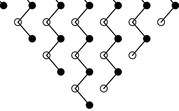 Figure 1
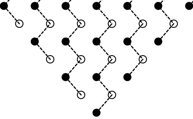 Figure 2
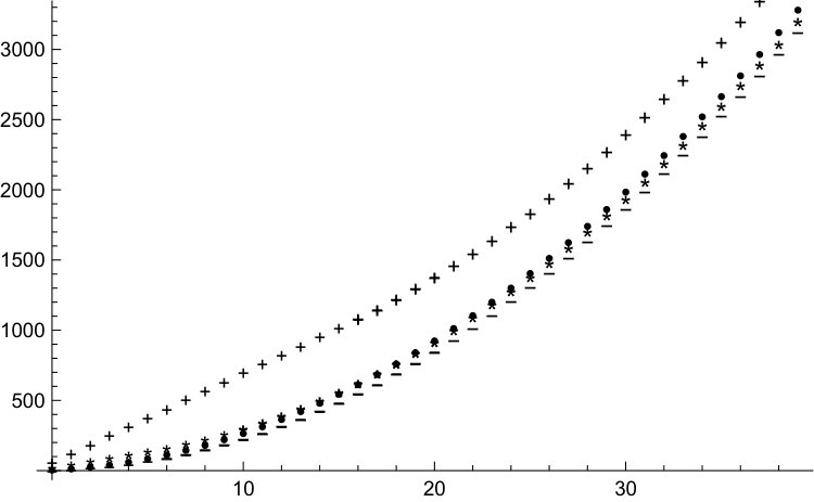 Figure 3
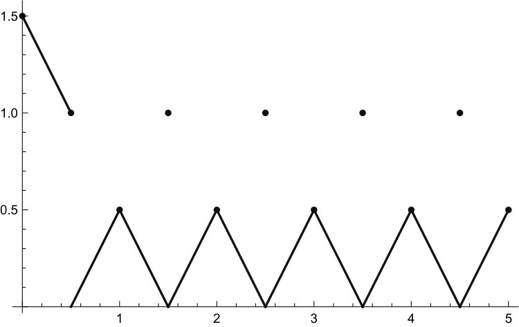 Figure 4
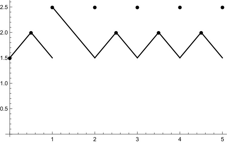 Figure 5
Peer Reviews
No public reviews on file for this paper yet. If you reviewed it on a platform where reviews are public (OpenReview, ICLR, NeurIPS, ICML), you can paste yours below so the community can read it here.
Videos
No videos yet. Explain this paper in a talk, walkthrough, or lecture? Add one.
Taxonomy
TopicsQuantum Mechanics and Non-Hermitian Physics · Nonlinear Waves and Solitons · Quantum chaos and dynamical systems
A three-dimensional superconformal quantum
mechanics with dynamical symmetry
Ivan E. Cunha and Francesco Toppan E-mail: [email protected]E-mail: [email protected]
Abstract
We construct a three-dimensional superconformal quantum mechanics (and its associated de Alfaro-Fubini-Furlan deformed oscillator) possessing an dynamical symmetry. At a coupling parameter the Hamiltonian contains a potential and a spin-orbit (hence, a first-order differential operator) interacting term. At four copies of undeformed three-dimensional oscillators are recovered. The Hamiltonian gets diagonalized in each sector of total and orbital angular momentum (the spin of the system is ). The Hilbert space of the deformed oscillator is given by a direct sum of lowest weight representations. The selection of the admissible Hilbert spaces at given values of the coupling constant is discussed. The spectrum of the model is computed. The vacuum energy (as a function of ) consists of a recursive zigzag pattern. The degeneracy of the energy eigenvalues grows linearly up to (in proper units) and quadratically for . The orthonormal energy eigenstates are expressed in terms of the associated Laguerre polynomials and the spin spherical harmonics. The dimensional reduction of the model to produces two copies (for and , respectively) of the two-dimensional deformed oscillator. The dimensional reduction to produces the one-dimensional deformed oscillator, with determined by .
CBPF, Rua Dr. Xavier Sigaud 150, Urca,
cep 22290-180, Rio de Janeiro (RJ), Brazil.*
CBPF-NF-002/19
1 Introduction
In this paper we construct a three-dimensional superconformal quantum mechanics having, as an input, an dynamical symmetry. The associated (denoted as “DFF”, see [1]) de Alfaro-Fubini-Furlan type of deformed oscillator, with as spectrum-generating superalgebra, is presented in detail. These quantum models (both the superconformal and the DFF one) are defined in terms of a dimensionless deformation parameter which, without loss of generality, can be assumed to belong to the interval. The undeformed DFF Hamiltonian corresponds to four copies of the three-dimensional isotropic oscillator; when , a spin-orbit term enters the Hamiltonians. It is a first-order differential operator which can be diagonalized in each sector of given total and orbital angular momenta.
The list of the main results is the following:
i) once derived the lowest weight representations, alternative admissible Hilbert spaces that can be associated with the quantum models at a given are constructed. Consistency conditions require the wave functions to be normalized and the Hamiltonian to be self-adjoint. The procedure is an extension of the approach and results discussed in [2, 3] for conformal quantum mechanics. The spectrum of the deformed oscillators is computed. When varying the deformation parameter (which, in physical applications, can play the role of an external control parameter) certain lowest weight representations of can be “switched on” as admissible in the given Hilbert space, while certain other lowest weight representations can be “switched off”. One of the consequences is the production, for the vacuum energies, of the recursive zigzag patterns observed in Figures 1 and 2;
ii) an unexpected feature concerning the degeneracy of the energy eigenvalues of the deformed oscillator is derived. For integer or half-integer the energy spectrum is a shifted version of the spectrum of the undeformed oscillator. The -deformed oscillator realizes an interpolation between two different regimes. Up to energy (measured in natural units, by setting , where is the energy difference between the first excited state and the vacuum) the degeneracy grows linearly, mimicking the behaviour of a two-dimensional oscillator; starting from , the degeneracy grows quadratically (we recall that the degeneracy of the -th excited energy eigenvalue of an ordinary -dimensional oscillator grows as ). This behaviour has been computed in Section 6 and visually presented in Figure 3;
iii) the orthonormal eigenstates are expressed in terms of two classical functions: the associated Laguerre polynomials dependent on the (square of) the radial coordinate and the spin spherical harmonics, see [4], dependent on the angular coordinates. This result has been derived in Appendix B, see formulas (B.34) and (B.36).
Besides the above points, further discussed features are the implementation of superselection rules, the recovery of lower-dimensional deformed oscillators via dimensional reduction and so on.
Conformal quantum mechanics was first introduced in [5]. The superconformal extension was presented in [6] and [7]. Superconformal quantum mechanics and its associated DFF deformed oscillators are a very active field of investigation with a growing body of literature. There are two main motivations for that. On one side, the development of sophisticated mathematical tools (e.g., for large -extended supersymmetry, the role of superconformal Lie algebras) to construct and explicitly solve models, both at the classical and quantum level. On a physical side, for its important applications. We mention in particular the motion of test particles in the proximity of the horizon of certain black holes, see [8] and the correspondence investigated in [9] and [10]. The holography has recently gained new attention in relation with the Sachdev-Ye-Kitaev models (see [11, 12] and references therein); in this context the connection between conformal and schwarzian mechanics is discussed, e.g., in [13, 14].
In the literature there are three main approaches to construct superconformal quantum mechanics. The most popular one consists in quantizing classical world-line superconformal sigma-models defined on supermultiplets of an -extended one-dimensional supersymmetry (for the relevant supermultiplets, see [15, 16], are of the type , corresponding to propagating bosonic fields, fermionic fields and auxiliary bosonic fields). In the sigma-model interpretation, is the dimensionality of the target manifold. These classical superconformal world-line sigma-models are constructed either via superspace (see the [17] review and the references therein; more recent works are [18, 19, 20, 21]) or via -module representations of one-dimensional superconformal algebras, as in [22, 23].
The so-called “triangular representations” (in contraposition to the ordinary “parabolic representations”) of superconformal algebras have been discussed in [24]. They induce the de Alfaro-Fubini-Furlan deformed oscillators counterparts of the superconformal mechanics. Some recent works on superconformal quantum mechanics, either “parabolic” or “trigonometric” cases, are [25, 26, 27, 28, 29, 30]. Particularly relevant for our purposes here is the [26] paper. There, it is shown that the quantization of world-line superconformal sigma-models with target dimensions cannot be performed straightforwardly, but require solving non-trivial non-linear equations. It is due to this obstruction that we apply here a more direct method (the second approach, pionereed in [28, 30] for one-dimensional models) to construct a three-dimensional superconformal quantum mechanics. It is rewarding that the dimensional reductions of the three-dimensional superconformal quantum mechanics allow to recover (see Section 7) the models obtained in [26] by quantizing the worldline superconformal sigma models based on the and the supermultiplets (for target dimensions , respectively). One sign of the obstruction for is the appearance in the Hamiltonian of the non-diagonal spin-orbit term.
The third approach to superconformal quantum mechanics is based on symmetries of the time-dependent Schrödinger equation, regarded as a partial differential equation (it will be briefly discussed in the Conclusions).
We mention that several different, both classical and quantum, supersymmetric models possessing (a real form of) as dynamical symmetry have been investigated in the literature, see [31, 25, 26, 32, 33, 29, 34]. These models do not correspond to the three-dimensional Hamiltonians here presented. The first one of these papers, [31], presents the dynamical symmetry of a Dirac magnetic monopole with a potential.
Hamiltonians with a spin-orbit coupling, as the one here discussed, are not a novelty. It has to be mentioned, in particular, the [35] paper. In that work a particular matrix Hamiltonian with spin-orbit coupling has been solved by showing that the system possesses an dynamical symmetry. The restriction to the upper left block of the matrix Hamiltonian (16) derived below produces, at the specific value, the Hamiltonian in formula (2.6) of [35] (a further constant , entering the (2.6) Hamiltonian, is set to zero). Since the coupling constant entering [35] is kept fixed, from that work no features can be derived concerning the zigzag pattern of vacuum energy or the interpolating regimes obtained at varying .
The scheme of the paper is the following. In Section 2 we introduce the three-dimensional superconformal quantum mechanics. In Section 3 we apply the de Alfaro-Fubini-Furlan “trick” to construct the associated deformed oscillator with spectrum-generating superalgebra. The selection of its admissible Hilbert spaces is discussed in Section 4. The derivation of its spectrum is given in Section 5. The computation of the energy degeneracy is presented in Section 6. The recovering of previous models from dimensional reduction is explained in Section 7. In the Conclusions we mention open problems and lines of future research. The paper is complemented by three Appendices. Our notations of conventions are introduced in Appendix A. In Appendix B the orthonormal eigenstates are computed. We illustrate in Appendix C the open problem of the reducibility of the Hilbert space with respect to the lowest weight representations versus its possible irreducibility with respect to a representation of a larger algebraic structure.
2 The three-dimensional superconformal quantum mechanics
We realize, following the approaches in [28] and [30], a superconformal dynamical symmetry in terms of first-order matrix differential operators. Several requirements have to be satisfied. The operators have to be Hermitian. The fermionic ones need to be block-antidiagonal in order to be accommodated into the odd sector of the superalgebra. A supersymmetric quantum mechanics has to be constructed at first. For our purposes the supersymmetry generators have to be the square roots of a Hamiltonian which corresponds to a deformation of the three-dimensional Laplacian of the free theory. It is easily seen that a three-dimensional Laplacian is nicely expressed in terms of quaternions (which require at least real matrices). On the other hand, as recalled in [30], the closure with Hermitian operators of a superconformal dynamical symmetry (which contains in particular the conformal partner of the Hamiltonian), requires the introduction of complex matrices. All in all, complex matrices is the minimal set-up to achieve the goal (it follows from the properties of Clifford algebras discussed, e.g., in [36] and [37]). It allows to produce an extended supersymmetric quantum mechanics, due to the presence of two block-antidiagonal matrices () which commute with the three imaginary quaternions (. An explicit realization of the matrices , and of the Fermion Parity Operator is given in (A.8). The two supersymmetry operators are further assumed to have scaling dimension if is the assigned scaling dimension of the three space coordinates (our notations and conventions are given in Appendix A).
A natural Ansatz to produce two supersymmetry operators with the required properties consists in setting
[TABLE]
In the above formula is a real parameter, is the radial coordinate, while and are introduced in (A.13).
The superalgebra of the supersymmetric quantum mechanics is
[TABLE]
The matrix supersymmetric Hamiltonian is given by
[TABLE]
where is the three-dimensional Laplacian and is the spin- introduced in (A.15). At the Hamiltonian gets reduced to . At non-vanishing two extra terms appear: a diagonal potential term proportional to in the upper/lower diagonal blocks and a non-diagonal spin-orbit interaction term proportional to . The latter one is a first-order differential operator.
The Hamiltonian has scaling dimension . Based on the de Alfaro-Fubini-Furlan construction [1], we can introduce its conformal partner as the rotationally invariant operator of scaling dimension . We can therefore set
[TABLE]
and verify whether the repeated (anti)commutators of the operators and close the one-dimensional superconformal algebra (see [38, 30] for a discussion of one-dimensional, -extended superconformal algebras). This is indeed the case. Four extra operators () have to be added. is the (bosonic) dilatation operator which, together with , close the subalgebra. The two fermionic operators , of scaling dimension , are introduced from the commutators . Finally, is the -symmetry bosonic operator of . It is introduced from the anticommutators with . The (anti)commutators among the eight operators close the superalgebra. We present them for completeness. The non-vanishing ones are
[TABLE]
with the antisymmetric tensor normalized so that .
Besides , , , respectively given in (1,5,6), the remaining operators are
[TABLE]
The Hamiltonian is, by construction, Hermitian. Since the spin is , the total angular momentum of the quantum-mechanical system is half-integer. The Hamiltonian is non-diagonal; on the other hand, due to the relation
[TABLE]
it gets diagonalized in each sector of given total and orbital angular momentum. In each such sector it corresponds to a constant kinetic term plus a diagonal potential term proportional to .
3 The three-dimensional deformed oscillator
By setting, following [1],
[TABLE]
with , respectively given in (5) and (6), we produce the matrix deformed oscillator Hamiltonian whose spectrum is discrete and bounded from below. By construction, the dynamical symmetry of the Hamiltonian acts as a spectrum-generating superalgebra for the Hamiltonian.
The explicit expression of is
[TABLE]
The spin of the quantum mechanical system is . Therefore, its total angular momentum is half-integer () and the relation with the orbital angular momentum is given by
[TABLE]
In the given sector, the operator from (14) is constant. We get
[TABLE]
Each given bosonic (or fermionic) energy eigenvalue in the sector is -times degenerated, the degenerate eigenstates being labeled by the quantum numbers .
The energy eigenstates of the system are described with the help of the two-component spin spherical harmonics, see [4], given by
[TABLE]
where (for ) are the ordinary spherical harmonics.
The spin spherical harmonics are the eigenstates for the compatible observable operators , , , with eigenvalues , , , respectively.
The spectrum of the model is derived from the creation (annihilation) operators (), with , which are introduced through the positions
[TABLE]
Indeed, we obtain
[TABLE]
together with
[TABLE]
For completeness we also present the commutators
[TABLE]
They should be compared with the analogous commutators for one-dimensional deformed oscillators (see [30]), producing deformed Heisenberg algebras with diagonal operators in the right hand side; the right hand side of (25) is diagonalized in the sector.
Let us set, for convenience, and . The explicit expression of the creation/annihilation operators is
[TABLE]
They can be factorized as
[TABLE]
The creation/annihilation operators anticommute with the Fermion Parity Operator ,
[TABLE]
producing towers of alternating bosonic/fermionic energy eigenstates.
A lowest weight state is defined to satisfy
[TABLE]
Due to the (27) factorization, in both cases, this is tantamount to satisfy .
A lowest weight representation is spanned by the action of the creation operators on .
If is either bosonic or fermionic, the vectors and , with belonging to the lowest weight representation, differ by a phase. Therefore, the action of , produces the same ray vector characterizing a physical state of the Hilbert space. This phenomenon was already observed [30] in the one-dimensional context. Without loss of generality we can just pick, let’s say, to create/annihilate the ray vectors.
We search for solutions of the lowest weight condition (29) of the form
[TABLE]
The sign of (no summation over this repeated index) refers to the bosonic (fermionic) states with respective eigenvalues () of the Fermion Parity Operator ; we have e_{+1}=\tiny{\left(\begin{array}[]{c}1\\ 0\end{array}\right)} and e_{-1}={\tiny{\left(\begin{array}[]{c}0\\ 1\end{array}\right)}}.
Solutions of (29) are obtained for the radial-coordinate functions given by
[TABLE]
where
[TABLE]
The corresponding lowest weight state energy eigenvalue from
[TABLE]
is
[TABLE]
Since does not depend on the quantum number , this energy eigenvalue is times degenerate.
We discuss in the next Section under which condition the vectors of a given lowest weight representation belong to a normed Hilbert space. For the time being we point out that the application of the creation operator on an energy eigenstate with energy eigenvalue produces a ray vector with energy eigenvalue . As we will see, an admissible Hilbert space is defined by a direct sum of (an infinite number of) lowest weight representations. The degeneracy of each energy level is finite and can be computed with a recursive formula. Let be the total number of distinct, admissible, lowest weight vectors in the Hilbert space and let be the number of degenerate eigenstates at energy level . At energy level we obtain
[TABLE]
The term in the right hand side gives the number of descendant states obtained by applying to the degenerate states at energy , while the term corresponds to the number of new primary states at . From (35), the computation of the degeneracy of the spectrum is reduced to a combinatorial problem based on the determination of the lowest weight vectors.
4 Alternative Hilbert spaces for the deformed oscillator
Without loss of generality we can restrict the real parameter to belong to the half-line since the mapping is recovered by a similarity transformation (induced by an operator ) which exchanges bosons into fermions. We have, indeed,
[TABLE]
At we recover four copies of the undeformed, isotropic, three-dimensional oscillator. Therefore, parametrizes the deformed oscillator.
To the following quantum numbers,
[TABLE]
is associated an lowest weight vector and its induced representation.
At a given , the Hilbert space has to be selected by requiring, in particular, the normalization of the wave functions entering a lowest weight representation. This puts restriction on the admissible lowest weight representations, the Hilbert space being constructed as the direct sum of the admissible lowest weight representations.
The analysis of [2, 3] (and also of [30]) can be extended to the present case. Two choices to select the Hilbert space naturally appear:
- •
case i: the wave functions can be singular at the origin, but they need to be normalized,
- •
case ii: the wave functions are assumed to be regular at the origin.
We will see in a moment that case i corresponds in restricting the admissible lowest weight representations to those satisfying the necessary and sufficient condition
[TABLE]
where was introduced in (31) and given in (32). The normalizability condition (38) is equivalent to the requirement
[TABLE]
for the lowest weight energy given in (34).
The case ii (regularity at the origin) corresponds in restricting the admissible lowest weight representations to those satisfying the condition
[TABLE]
The single-valuedness of the wave functions at the origin implies that the equality can only be realized with vanishing () orbital angular momentum (therefore, for and ). At one recovers the vacuum state of the undeformed oscillator. For the deformed oscillator the strict inequality
[TABLE]
is required as necessary and sufficient condition.
For illustrative purposes it is useful to present a table (up to ) of the range of admissible lowest weight representations under norm (case i) and reg (case ii) conditions. The quantum numbers are respectively given in columns , while and are presented in columns and . We have
[TABLE]
For the undeformed oscillator, the restrictions from either case i or case ii select the same Hilbert space. It is the direct sum of all lowest weight representations with satisfying (37), while is restricted to be
[TABLE]
For the deformed oscillators, the Hilbert spaces and are direct sums of the lowest weight representations with satisfying (depending on , )
[TABLE]
The vacuum energy of the system is obtained by comparing the smallest lowest weight energies (obtained from (34)) in each one of the three contributing sectors ( with , with , with ) for the admissible values of . One should take into account that for , at a given , the smallest value of energy is encountered at the smallest admissible value of . Conversely, for , , the smallest lowest weight energy is encountered at the largest admissible value of .
The normalizability condition (38) comes from the requirement to have a finite norm for the lowest weight vector (30), such that
[TABLE]
Passing to spherical coordinates, the only potentially troublesome integral is
[TABLE]
which is finite at the origin, provided that , namely the (38) condition. A simple inspection shows that, acting with the creation operators, no further condition is necessary to ensure the normalizability of the excited states of the lowest weight representation.
The normalizability condition discussed in the [2, 3, 30] papers (which deal with one-dimensional systems) implies that the normalized wave functions are defined on the real line, with the possible “smooth” singularity at the origin. The regular wave functions (for ) are, on the other hand, defined on the half line and satisfy the Dirichlet boundary condition at the origin. We stress that the mathematical framework in the present work coincides with the one introduced in [2, 3, 30]. For the singular Hilbert space this means that one can extend the wavefunctions (defined by the spherical coordinates ) in two regions, namely (parametrized by ) and (parametrized by ), so that their intersection is the origin. Mathematically, this construction works fine. On a physical ground one has to reconcile the interpretation of the wavefunctions defined on with the wavefunctions defined on the ordinary three-dimensional space. This can be achieved by taking into account that the transformation
[TABLE]
is a symmetry of the Hamiltonian. The induced operator , acting on the wavefunctions defined on , satisfies the
[TABLE]
condition, is Hermitian and possesses eigenvalues, provided that
[TABLE]
implying that (and consequently ) is an integer. If (67) is satisfied for the lowest weight vector, and (66) are satisfied for all states belonging to the associated lowest weight representation. For such a well-defined operator, one can impose the coset construction, by identifying
[TABLE]
Under this coset construction, one can set
[TABLE]
The coset construction entails, from equations (67) and (32), the quantization of which, under this condition, is restricted to be integer
[TABLE]
We stress the fact that the Hilbert space can be consistently defined for any real value of . It is the coset construction with the associated interpretation which requires to be an integer.
5 The spectrum of the -deformed oscillator
In this Section we present, for , the computation of the spectrum for the alternative choices of and Hilbert spaces. Without loss of generality is taken to be . We start with the case (normalized wave functions).
5.1 The spectrum for the Hilbert space of normalized wave functions
For it is convenient to introduce, via the floor function, the parameter , defined as
[TABLE]
The results for the spectrum split into six different cases which have to be separately analyzed:
- •
case I: (the undeformed oscillator),
- •
case II: , with (),
- •
case III: , with ,
- •
case IV: ,
- •
case V: , therefore , with ,
- •
case VI: , therefore , with .
The energy eigenvalues corresponding to the above cases are
- •
case I: , where is a non-negative integer.
The vacuum energy is ; the ground state is four times degenerated, with two bosonic and two fermionic eigenstates (hence “”).
The vacuum lowest weight vectors are specified by the quantum numbers , , and (here and in the following) all compatible values .
- •
case II: , with .
The vacuum energy is ; the degeneration of the ground state is , with bosonic and fermionic eigenstates, and is therefore denoted as “”.
The vacuum lowest weight vectors are specified by , with either , or , .
- •
case III: , with .
The vacuum energy is ; the degeneration of the ground state is , with bosonic and fermionic eigenstates, and is therefore denoted as “”.
For the two vacuum lowest vectors are specified by , , .
For the vacuum lowest vectors are specified either by , , or by , , .
- •
case IV: two series of energy eigenvalues , with , are encountered.
The vacuum energy is ; the ground state is fermionic and doubly degenerated (“”).
The two vacuum lowest weight vectors are specified by , , .
- •
case V: two series of energy eigenvalues , , with , are encountered.
The vacuum energy is ; the ground state is bosonic and -times degenerated (hence “”).
The vacuum lowest weight vectors are specified by , , .
- •
case VI: two series of energy eigenvalues , , with , are encountered.
The vacuum energy is ; the ground state is fermionic and -times degenerated (hence “”).
The vacuum lowest weight vectors are specified by , , .
[TABLE]
There is an important remark. The energy spectrum of the V and VI cases coincides under a
[TABLE]
duality transformation. Under this duality transformation the parity (bosonic/fermionic) of the ground state is exchanged. On the other hand, the degeneracies of the energy eigenvalues above the ground state are not respected by the duality transformation. It is sufficient to discuss a specific example to show it. Let’s take with and consider the dually related and cases.
The lowest weight vectors appearing in the first five energy levels (from the vacuum energy to ) are presented in the following table
[TABLE]
The lowest weight vectors are identified by their quantum numbers , the sign referring to , while (standing for bosons) and (standing for fermions) correspond to , , respectively.
The degeneracy of a given energy level is computed with the recursive formula (35) involving primary (lowest weight vectors) and descendant states. The results are presented in the table
[TABLE]
One can see that is the first energy level where an inequality of the degeneracies is produced
[TABLE]
The -dependence of the vacuum energy is graphically presented in Figure 1.
5.2 The spectrum for the Hilbert space of regular wave functions
The case was already discussed since, for this value, the and Hilbert spaces coincide. For the following cases have to be separately treated:
- •
case i: ,
- •
case ii: ,
- •
case iii: ,
- •
case iv: ,
- •
case v: , with ,
- •
case vi: ,
- •
case vii: ,
- •
case viii: , with and ,
- •
case ix: , with ,
- •
case x: , with and ,
- •
case xi: , with .
The energy eigenvalues corresponding to the above cases are
- •
case i: two series of energy eigenvalues, and , with , are encountered.
The vacuum energy is ; the ground state is bosonic and doubly degenerate (hence, denoted as “”).
The vacuum lowest weight vectors are specified by the quantum numbers , .
- •
case ii: the energy eigenvalues are , with .
The vacuum energy is ; the degeneration of the ground state is , with bosonic and fermionic eigenstates (“”).
The vacuum lowest weight vectors are specified by , with and by with and .
- •
case iii: two series of energy eigenvalues, and , with , are encountered.
The vacuum energy is ; the ground state is fermionic and times degenerate (“”).
The vacuum lowest vectors are specified by , , .
- •
case iv: the energy eigenvalues are , with .
The vacuum energy is ; the degeneration of the ground state is , with bosonic and fermionic eigenstates (“”).
The vacuum lowest weight vectors are specified by , with and by with and .
- •
case v: two series of energy eigenvalues , , with , are encountered.
The vacuum energy is ; the ground state is fermionic and times degenerate (“”).
The vacuum lowest weight vectors are specified by , , .
- •
case vi: the energy eigenvalues are , with .
The vacuum energy is ; the degeneration of the ground state is fermionic and times degenerate (“”).
The vacuum lowest weight vectors are specified by with and .
- •
case vii: the energy eigenvalues are , with .
The vacuum energy is ; the ground state is fermionic and times degenerate (“”).
The vacuum lowest weight vectors are specified by , with and .
- •
case viii: two series of energy eigenvalues , , with , are encountered.
The vacuum energy is ; the ground state is bosonic and degenerate (“”).
The vacuum lowest vectors are specified by , with and .
- •
case ix: the energy eigenvalues are , with .
The vacuum energy is ; the degeneration of the ground state is with bosonic and fermionic eigenstates (“”).
The vacuum lowest weight vectors are specified by with and and by , with and .
- •
case x: two series of energy eigenvalues , , with , are encountered.
The vacuum energy is ; the ground state is fermionic and degenerate (“”).
The vacuum lowest vectors are specified by , with and .
- •
case xi: the energy eigenvalues are , with .
The vacuum energy is ; the degeneration of the ground state is with bosonic and fermionic eigenstates (“”).
The vacuum lowest weight vectors are specified by with and and by , with and .
[TABLE]
The -dependence of the vacuum energy is graphically presented in Figure 2.
5.3 About superselecting the wave functions
It is beyond the scope of this work to present an investigation of the admissible superselection rules which can be implemented on the and Hilbert spaces. We limit ourselves to mention here a natural type of superselection for its consequence on the spectrum. As we have seen, when the deformation parameter is integer or half-integer, the spectrum coincides with a shifted version of the undeformed oscillator (more on that in Section 6). A natural superselection consists in imposing the ground state and the even excited states to be bosonic, with fermionic odd excited states (or viceversa, exchanging the role of bosons and fermions). For or this superselection is implemented by the projectors
[TABLE]
where denotes the given ground energy. The “” (“”) sign is associated with the fermionic (bosonic) ground state. The superselected wave functions are constrained to satisfy
[TABLE]
6 Combinatorics of the energy eigenstates degeneracy
For integer or half-integer the spectrum of the deformed oscillator is a shifted version of the undeformed oscillator. A second dissimilarity consists in the different degeneracies of the energy eigenvalues for the corresponding ground states and excited states. When , the spectrum is a combination of two differently shifted spectra of the undeformed oscillator (see cases IV, V, VI in (LABEL:normcases) and cases i, iii, v, viii, x in (LABEL:regcases)).
In order to facilitate the comparison with the undeformed oscillator and highlight the differences, for integer and half-integer we solve the combinatorics of the degenerate eigenstates provided by the (35) recursive relation with the (62) input of primary (i.e. lowest weight vectors) states. The same technique can be applied for any real value of (the results for this latter case will not be reported to avoid eccessively burdening the paper).
Let and denote the energy eigenvalues for integer or half-integer in correspondence with, respectively, the and choices of the Hilbert space (, are the corresponding vacuum energies). The energy shifts , with respect to the undeformed oscillator can be read from Figures 1 and 2. We have
[TABLE]
with, for ,
[TABLE]
We start our analysis of the eigenvalue degeneracies by recalling, at first, the features of the undeformed oscillator.
6.1 Degeneracies of the undeformed oscillator
Since, at , the (16) Hamiltonian corresponds to four copies of the ordinary isotropic three-dimensional oscillator, its degeneracy is
[TABLE]
Here denotes the eigenvalues degeneracy of the ordinary three-dimensional oscillator. It produces the tower of states, the vacuum being non-degenerate.
The rotational invariance of the ordinary three-dimensional oscillator implies that at each energy level the degenerate states can be accommodated into multiplets (denoted as “”) of non-negative integer orbital angular momentum , each multiplet containing states. We get, at the lowest orders,
[TABLE]
The spectrum of the ordinary oscillator can be recovered by imposing, to the Hamiltonian at , two independent superselection rules defined by the Fermion Parity Operator and by the spin operator (since the spin-orbit coupling is absent at , for this particular value of the Hermitian operator commutes with the Hamiltonian). The corresponding projector operators , which induce the superselection rules are different from the projectors introduced in (92); they are given by
[TABLE]
and satisfy
[TABLE]
The two compatible superselection rules at can be imposed by restricting the wave functions to satisfy
[TABLE]
One should note that the rotational invariance is, from the spectrum-generating superalgebra viewpoint, an emergent symmetry, being not immediately derivable from the data.
6.2 Degeneracies for and with Hilbert space
We present here the results of the degeneracies for the Hilbert space of normalized wave functions. We have
Case a: (energy levels ) with .
For the degeneracy of the level is simply
[TABLE]
The above formula can be recovered from the following most general case at given integer . The degeneracy grows linearly (mimicking a two-dimensional oscillator) up to ; it then grows quadratically starting from :
[TABLE]
Case b: (energy levels ) with .
As in the previous case, the degeneracy grows linearly (mimicking a two-dimensional oscillator) up to ; it then grows quadratically starting from :
[TABLE]
We provide in Figure 3 a graphical description of the degeneracy.
6.3 Degeneracies for and with Hilbert space
We present here the results of the degeneracies for the Hilbert space of regular wave functions. We have
Case a: half-integer with energy levels .
The and cases present the same degeneracy, the functions , being given by
[TABLE]
The case can also be recovered from the most general formula for , with . We have
[TABLE]
We recover the same feature observed for normalized wave functions belonging to , namely a linear growth followed by a quadratic growth.
Case b: integer with energy levels .
The and cases present the same degeneracy, the functions , being given by
[TABLE]
The case can also be recovered from the most general formula for , with . We have
[TABLE]
Here again we observe a linear growth up to , followed by a quadratic growth.
7 Dimensional reductions of the deformed oscillator
In this Section we discuss how to recover two-dimensional and one-dimensional models of superconformal quantum mechanics (originally introduced in [26] via the quantization of worldline superconformal sigma-models, with two and one target coordinates, respectively) by dimensional reduction of the three-dimensional superconformal quantum mechanics. We explicitly treat the case of the de Alfaro-Fubini-Furlan deformed oscillator (the construction can be repeated step by step, with analogous results, in the absence of the oscillatorial term).
7.1 The dimensional reduction
To obtain this dimensional reduction we have to freeze the dependence on the third coordinate in the wave functions. This can be achieved by setting , , entering the operators (1,5,6,2) to be restricted to
[TABLE]
(the last equality holds for in formula (2)). With the above positions the (anti)commutators (12) are maintained. The operator entering the Hamiltonians (5) and (16) is now given by . In the two-dimensional case, being proportional to , this operator is diagonal.
The resulting Hamiltonian of the deformed oscillator corresponds to two copies of the two-dimensional matrix Hamiltonians derived in [26] from the quantization of the worldline sigma-model with two propagating bosonic and two propagating fermionic fields. We have
[TABLE]
The two non-vanishing upper-left and bottom-right blocks of the given Hamiltonian present the deformation parameters and , respectively.
There is an important remark. For the deformed oscillator, the spectrum-generating superalgebra induced by the (1,5,6,2) operators with the (114) restriction does not coincide with the spectrum-generating superalgebra introduced in [26]. The reason is that the ladder operators constructed with and connect the upper-left and bottom-right blocks, while the ladder operators of [26] act inside each component blocks. Therefore, the spectrum-generating superalgebra of [26], as well as its charge-conjugated superalgebra (also in [26]) are, from the point of view of the dimensionally reduced theory, emergent spectrum-generating superalgebras which are not directly connected with the original superalgebra.
7.2 The dimensional reduction
To operate this dimensional reduction it is convenient to freeze the dependence on the , coordinates by setting
[TABLE]
The (1,5,6,2) operators continue, with the above positions, to satisfy the (anti)commutators (12). The resulting deformed oscillator, given by (we set, for simplicity, )
[TABLE]
coincides with the model derived in [26] from the quantization of the world-line sigma model induced by the supermultiplet (namely, with one propagating boson, four propagating fermions and three auxiliary fields). The Hamiltonian possesses the larger spectrum-generating superalgebra, with . On the other hand, as recalled in [30], the generators are sufficient to determine the ray vectors of the Hilbert space (the vectors produced by the remaining generators differ by an inessential phase). From the dimensional reduction viewpoint, the extra generators entering are associated with an emergent symmetry, not manifest from the construction.
8 Conclusions
We provided a direct construction of a three-dimensional superconformal quantum mechanics and of its associated de Alfaro-Fubini-Furlan deformed oscillator. Our approach allowed to overcome the difficulties (pinpointed in [26]) in quantizing worldline superconformal sigma-models with target dimensions. It is rewarding that a dimensional reduction of the model allows to recover the quantized worldline superconformal sigma-models introduced in [26]. For the deformed oscillator, acts as a spectrum-generating superalgebra; the complete spectrum is obtained from a (infinite) direct sum of lowest weight representations. Depending on the coupling constant , different Hilbert spaces can be consistently selected by suitably restricting the allowed lowest weight representations.
Even if is sufficient to completely determine the spectrum, extra symmetries can play a role (possibly as enhanced symmetries at given values of the coupling constant ). This is worth investigating since the recalled arbitrariness in the selection of the Hilbert space can be eliminated if an enlarged algebra is responsible for extra conditions to be imposed.
In this paper we were able to determine the three-dimensional quantum Hamiltonians (given in (5) and (16) for the superconformal and, respectively, deformed oscillator cases). Once the Hamiltonian has been individuated, there is a standard method to be applied (see [39]) to derive the symmetry operators of the associated partial differential equation (for the case at hand, the partial differential equation is the time-dependent Schrödinger equation for the given Hamiltonian). By applying this method, the most general dynamical symmetry of the model can be derived through a very lengthy, but straightforward procedure. We plan to address this investigation in a future work. It allows to answer the open question about the possible existence of extra symmetries and of the role they could play. It is worth mentioning that a similar analysis, conducted for a one-dimensional superconformal quantum mechanics, led to the surprising result [40] that the higher-spin superalgebra [41] is a dynamical symmetry of the model. A tantalizing possibility is that the extra symmetries, as those mentioned in Appendix C, of the superconformal quantum mechanics could be linked to a BMS/CFT correspondence (see [42]), the BMS transformations being associated with the “large” diffeomorphisms acting on asymptotically flat space-times [43].
Appendix A: notations and conventions
We collect here for convenience the relevant notations and conventions used throughout the paper.
The Identity matrix is denoted as “”. The three Pauli matrices are
[TABLE]
The following complex matrices () are introduced:
[TABLE]
The matrices are block-antidiagonal, while is the Fermion Parity Operator which defines bosons and fermions as its eigenvectors with eigenvalues and , respectively. When we need to stress this property, we use the notation
[TABLE]
The imaginary unit “” is introduced in the definition of the matrices , so that they furnish a representation of the three imaginary quaternions. Indeed, the composition law
[TABLE]
is satisfied. The totally antisymmetric tensor is normalized so that . Throughout the paper the Einstein convention of summation over the repeated indices is understood unless otherwise specified.
By construction, the matrices commute with the quaternionic matrices :
[TABLE]
In Cartesian coordinates the position vector has components . The orbital angular momentum has components , where
[TABLE]
For convenience, we introduced the slashed notation for the Euclidean version of the Dirac’s operator and a matrix-valued space coordinates operator, by setting
[TABLE]
It follows, in particular, that and , where is the radial coordinate. In our conventions the spherical coordinates (restricted to , , ) are introduced through the positions
[TABLE]
The spin has components , so that
[TABLE]
Appendix B: the orthonormal eigenstates
We present for completeness the orthonormal eigenstates. The derivation of the orthonormal conditions is based on some key observations and a lengthy, but straightforward inductive proof concerning the excited states. We outline the main points and give the final results.
At first one has to mention that the spin spherical harmonics introduced in (21) are orthonormal, satisfying
[TABLE]
with an infinitesimal solid angle.
By setting , the integral (64) produces a Gamma function, so that
[TABLE]
The lowest weight vectors from (30) which satisfy, at given , the (29) condition are orthogonal. The orthonormal wave functions are expressed in terms of the normalizing factor . We have
[TABLE]
so that
[TABLE]
The excited eigenstates , obtained by applying times the creation operator (26), are orthogonal, as it can be easily verified. The computation of their normalization factors which make the wave functions orthonormal is more cumbersome. It involves the computation of Rodrigues-type formulas, see [44], for recursive polynomials in the radial coordinate . These recursive polynomials can be recovered from the associated Laguerre’s polynomials. In order to proceed we recall that
[TABLE]
and that the (unnormalized) lowest weight vectors from (30) are
[TABLE]
The action of can be read from equation (14), while the action of can be read from the
[TABLE]
identity. The even and odd excited states are therefore respectively given by
[TABLE]
where and are -dependent polynomials recursively determined by the Rodrigues-type formulas
[TABLE]
where, see (32),
[TABLE]
The connection with the associated Laguerre’s polynomials is as follows (we discuss it explicitly for the even polynomials , the derivation for the odd polynomials is made along the same lines). We obtain, from (B.14), the relation
[TABLE]
It follows in particular, from , that
[TABLE]
The associated Laguerre polynomials are introduced through the position
[TABLE]
They satisfy the identities
[TABLE]
Since
[TABLE]
by setting
[TABLE]
we can identify
[TABLE]
By assuming the Ansatz
[TABLE]
after lengthy computations and the use of the (8) identities, one arrives at the inductive proof that (B.30) is satisfied, provided that
[TABLE]
The even and odd polynomials are expressed, in terms of the associated Laguerre polynomials, as
[TABLE]
By plugging these expressions into the (8) formulas we are able to determine the normalizing factors that need to be used to construct orthonormal excited eigenstates. The normalizing factors are recovered from the orthogonal relations for the associated Laguerre polynomials, given by
[TABLE]
The final expressions for the orthonormal wave functions are
[TABLE]
with
[TABLE]
and
[TABLE]
with
[TABLE]
The parameter was introduced in (B.22). One should note that reproduces, as it should be, the normalizing factor given in formula (B.3).
Appendix C: a graphical illustration of an open problem
The three dimensional deformed oscillator can be completely solved, its energy spectrum and associated degeneracy computed. On the other hand, as discussed in Sections 5 and 6, alternative admissible choices of Hilbert space lead to different results corresponding to different quantum models. This means that the spectrum-generating superalgebra provides a (relevant) piece of information, but it does not allow to uniquely deduce the spectrum and the degeneracy of the -deformed model. Some extra information should be supplemented. It is quite possible that (yet to be understood) larger algebraic structures could be responsible for that, in such a way that they allow to uniquely pinpoint a given quantum model. The source of this ambiguity is the fact that the Hilbert space is not expressed by a single irreducible representation, but by a direct sum of several (infinite) lowest weight representations of the spectrum-generating superalgebra. Consistent selections of subsets of the set of lowest weight representations therefore lead to different Hilbert spaces.
The open problem of searching for enlarged algebraic structures is not specific to the three-dimensional deformed oscillator; it applies to the whole class of related (deformed) oscillators. It already appears in the case of the two-dimensional oscillator which corresponds, see formula (115), to a dimensional reduction of the oscillator. It is quite appealing to focus on this simpler case because it offers a nice graphical visualization of the question at hand.
For our illustrative purpose it is sufficient to take a superselected version of the undeformed two-dimensional theory with a unique bosonic vacuum and integerly-spaced energy excited states (the energy degeneracy growing linearly) arranged in a triangular shape as shown in Figures 4 and 5 below. As discussed in Section 3, the ray vectors are determined by the spectrum generating subalgebra (the action of the remaining generators produce inessential phases). In [26] it was shown that a new set of operators, obtained by conjugating the original operators of the spectrum-generating superalgebra, produce another superalgebra, denoted as . The details of the [26] construction are not relevant here. What is relevant is that the conjugated operators admit a nice “mirror” interpretation, visualized in Figure 5. The huge Enveloping Algebra induced by the operators entering both and uniquely determines the spectrum of the theory, as explained in the comment about Figure 5.
An enlarged algebraic structure, producing the three-dimensional counterpart of this simpler two-dimensional setting, has to be properly investigated.
Acknowledgments
The authors are grateful to Naruhiko Aizawa and Zhanna Kuznetsova for helpful discussions. This work is supported by CNPq (PQ grant 308095/2017-0).
The reference list from the paper itself. Each links out to its DOI / PubMed record.
- 1[1] V. de Alfaro, S. Fubini and G. Furlan, Nuovo Cim. A 34 (1976) 569.
- 2[2] H. Miyazaki and I. Tsutsui, Ann. Phys. 299 (2002) 78; ar Xiv:quant-ph/0202037.
- 3[3] L. Fehér, I. Tsutsui and T. Fülöp, Nucl. Phys. B 715 (2005) 713; ar Xiv:math-ph/0412095. 3; ar Xiv:1112.0995[hep-th].
- 4[4] L. C. Biedenharn and J. D. Louck, Angular momentum in Quantum Physics: Theory and Application , in Encycl. of Mathematics 8 , Reading, Addison-Wesley (1981) p. 283, ISBN 0-201-13507-8.
- 5[5] F. Calogero, J. Math. Phys. 10 (1969) 2191.
- 6[6] S. Fubini and E. Rabinovici, Nucl. Phys. B 245 , (1984) 17.
- 7[7] V. P. Akulov and A. I. Pashnev, Theor. Math. Phys. 56 (1983) 862 [Teor. Mat. Fiz. 56 (1983) 344].
- 8[8] R. Britto-Pacumio, J. Michelson, A. Strominger, and A. Volovich, Lectures on superconformal quantum mechanics and multi-black hole moduli spaces , in Progress in String Theory and M-Theory, NATO Science Series Vol. 564 , Kluwer Acad. Press (2001) 235; ar Xiv:hep-th/9911066.