Turbulent effects through quasi-rectification
Remi Carles, Christophe Cheverry

TL;DR
This paper presents a realistic model explaining how electromagnetic waves are generated, propagate, and interact in strongly magnetized plasmas or NMR, highlighting turbulence through wave interference over long times.
Contribution
It introduces a new model for wave interactions in magnetized plasmas and NMR, emphasizing turbulence effects from wave interference over extended periods.
Findings
Electromagnetic waves can be internally generated and interact in magnetized plasmas and NMR.
Wave interference leads to turbulence phenomena over long times.
The model captures nonlinear and dispersive effects in high-frequency solutions.
Abstract
This article introduces a physically realistic model for explaining how electromagnetic waves can be internally generated, propagate and interact in strongly magnetized plasmas or in nuclear magnetic resonance experiments. It studies high frequency solutions of nonlinear hyperbolic equations for time scales at which dispersive and nonlinear effects can be present in the leading term of the solutions. It explains how the produced waves can accumulate during long times to produce constructive and destructive interferences which, in the above contexts, are part of turbulent effects.
Click any figure to enlarge with its caption.
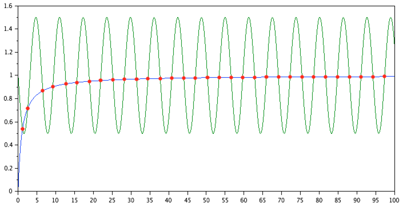 Figure 1
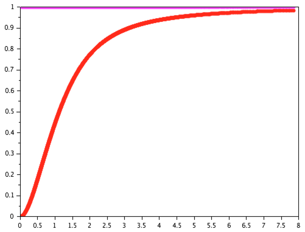 Figure 2
Peer Reviews
No public reviews on file for this paper yet. If you reviewed it on a platform where reviews are public (OpenReview, ICLR, NeurIPS, ICML), you can paste yours below so the community can read it here.
Videos
No videos yet. Explain this paper in a talk, walkthrough, or lecture? Add one.
Taxonomy
TopicsAdvanced Mathematical Physics Problems · Quantum chaos and dynamical systems · Nonlinear Waves and Solitons
Turbulent effects
through quasi-rectification
Rémi Carles
[email protected] http://carles.perso.math.cnrs.fr/ and
Christophe Cheverry
[email protected] https://perso.univ-rennes1.fr/christophe.cheverry Univ Rennes, CNRS
IRMAR - UMR 6625
F-35000 Rennes
France
Abstract.
This article introduces a physically realistic model for explaining how electromagnetic waves can be internally generated, propagate and interact in strongly magnetized plasmas or in nuclear magnetic resonance experiments. It studies high frequency solutions of nonlinear hyperbolic equations for time scales at which dispersive and nonlinear effects can be present in the leading term of the solutions. It explains how the produced waves can accumulate during long times to produce constructive and destructive interferences which, in the above contexts, are part of turbulent effects.
Keywords. Nonlinear geometrical optics; oscillatory integrals; dispersion; interferences; turbulence; magnetized plasmas; nuclear magnetic resonance.
Contents
1. Introduction
In this introduction, we present the main aspects of our text. In Subsection 1.1, we introduce a simple ODE model that is intended to serve as a guideline. In Subsection 1.2, we extend this model to better incorporate important specificities of two realistic situations which are related to strongly magnetized plasmas (SMP) and nuclear magnetic resonance (NMR). In Subsection 1.3, we state under simplified assumptions our two main results, Theorems 1.3 and 1.4. We also give an overview of our article.
1.1. A toy model
Introduce the phase given by
[TABLE]
Let be a small parameter, and . Fix numbers such that . Select and . Then, define
[TABLE]
Definition 1.1**.**
The number is called the gauge parameter associated with .
Consider the ordinary differential equation on the complex plane given by
[TABLE]
We can study the equation (1.3) on three different time scales:
Fast, when , that is when undergoes a few number of oscillations;
Normal, when , that is when generates oscillations, whereas the periodic part () inside sees a few number of oscillations;
Slow, when or , that is when involves oscillations.
In this subsection, we analyze (1.3) during long times or . With this in mind, we can change according to
[TABLE]
Expressed in terms of , the equation (1.3) becomes
[TABLE]
The initial data is still zero. Denote by the solution corresponding to the linear evolution, that is the solution obtained from (1.5) when . When and when , the solution to (1.5) looks like . Our aim is to first study the expression . Then, we incorporate nonlinear effects by looking at a critical size for the nonlinearity, corresponding to the special case and . This means to single out the following equation
[TABLE]
The integral formulation of (1.6) reads
[TABLE]
In Paragraph 1.1.1, we first show that , an estimate which is sharp when . As a consequence, the nonlinear contribution brought by the integral term inside (1.7) is likely to be of the same order of magnitude as the linear one. It can be expected that . In Paragraph 1.1.2, we prove that this is indeed the case if and only if .
1.1.1. The linear case
By construction, we have
[TABLE]
We start the analysis of (1.7) by looking at the part through the expression of (1.8). Examine the right hand side of (1.8). For harmonics with , since , remark that
[TABLE]
Exploiting (1.9), a single integration by parts yields
[TABLE]
In other words, assuming that , we find
[TABLE]
The situation is completely different when . Fix an integer . The solution computed at the time can be viewed as a sum of contributions produced over time by the source term, namely
[TABLE]
Since the function is periodic of period , the wave packets can be interpreted according to with
[TABLE]
The function has exactly two non-degenerate stationary points in the interval , at the positions and . Using the periodicity to get rid of the boundary terms and applying stationary phase formula, it follows that
[TABLE]
Let be such that
[TABLE]
Observe that
[TABLE]
The combination of (1.11), (1.14) and (1.15) indicates that, when , wave packets of amplitude are repeatedly created over time when solving (1.3) in the case .
Look at (1.11). The emitted signals (one per period ) have cumulative effects up to the stopping time . They give rise to a growth rate with respect to the time variable . For long times , assuming that , we can assert that
[TABLE]
This short discussion about the linear situation () highlights a difference between the cases
- see (1.10) - and - see (1.16). This observation is important in the perspective of nonlinear effects. As a matter of fact, it allows a first selection between the different modes .
1.1.2. Nonlinear effects
Here, we consider the nonlinear framework, when and . The difference is subject to
[TABLE]
Using a Picard scheme, it is easy to infer that the life span of the solution to the integral equation (1.17), and therefore of the solution to (1.6), can be bounded below by a positive constant not depending on . Knowing (1.10) and (1.16), it is also possible to deduce that is of size when , and of size when . This means that the preceding dichotomy between the two cases and remains when .
Fact 1**.**
When solving (1.6), the harmonic stands out from the others. Given , we find when , and when .
Assume that . The identity (1.7) becomes after an integration by parts
[TABLE]
From the equation (1.6), since we have seen that the solution is (at least) bounded, we know that . From (1.18), it follows that
[TABLE]
Now, assume that and moreover that . To show that, in this situation, nonlinear effects actually occur, it suffices to produce an example. To this end, take and , so that . Choose . Then, using (1.16), the identity (1.7) becomes
[TABLE]
This implies that , and therefore
[TABLE]
In view of the above formula, the asymptotic behavior of the nonlinear solution can strongly differ from the one of the linear solution .
Fact 2**.**
When solving (1.6), the gauge parameter stands out from the others. When , the asymptotic behaviors of and when goes to [math] are the same. On the contrary, when , nonlinear effects can be expected at leading order.
1.2. A more realistic model
The preceding features, Facts 1 and 2, which have been emphasized in the case of ODEs, are still present when dealing with partial differential equations arising in strongly magnetized plasmas (SMP) or in nuclear magnetic resonance experiments (NMR). But, there are two emerging issues: the first is due to dispersive effects which are completely absent in the ODE case; the second comes from the occurrence of non-trivial spatial variations when dealing with the phase . At all events, the discussion becomes much more subtle, and new important phenomena can and do occur.
In order to investigate SMP or NMR, we must consider the PDE counterpart of (1.3), which is
[TABLE]
where and . The state variable is and . The action of the pseudo-differential operator is given on the Fourier side by the multiplier .
In what follows, we will focus on the scalar wave equation (1.20). The origin of equation (1.20), its physical significances and the reasons why it may be seen as a universal problem (when dealing with systems of hyperbolic equations) will be clearly explained in Sections 2 and 3. We will work in space dimension one. The possible multidimensional effects will not be investigated here.
We now fix some notations and we introduce simplified assumptions intended to facilitate the presentation of our main results. We suppose that the symbol is smooth, say . The function is even. It is such that for some . It is strictly increasing on . Moreover, for large values of , it is subject to
[TABLE]
as well as
[TABLE]
Fix some . The source term is defined by
[TABLE]
In (1.23), the amplitudes are chosen in the set of smooth functions whose all derivatives are bounded. They are selected in such a way that, for some and some with , we have
[TABLE]
The amplitude is chosen periodic for large times in the second variable. In other words, there exists and a smooth function such that
[TABLE]
The phase arising in (1.23) is more general than in (1.1). It does depend on the spatial variable . It is the sum of a quadratic part (in and ) and a periodic part (in ).
Assumption 1.2** (Selection of a relevant phase ).**
The function is
[TABLE]
In Section 2, the above assumptions on and will be motivated by the study of two realistic situations which are related to strongly magnetized plasmas (SMP) and nuclear magnetic resonance (NMR). In Section 3, to better incorporate important specificities of SMP and NMR, they will be somewhat generalized.
In the right hand side of (1.20), the nonlinear part is, up to some localization in time and space, of the same form as in the previous subsection. Select a nonnegative cut-off function which is equal to in a neighborhood of the origin and which is such that . Fix some parameter which is aimed to measure the strength of the spatial localization. We impose
[TABLE]
Taking into account the conditions on the support of the ’s and , the term becomes effective only for , that is after the term has played its part. So we observe successively two distinct phenomena: a possible linear amplification, and then nonlinear interactions.
The solution to (1.20) exists on a time interval with . The argument is similar to the one given for the toy model. Through the change (1.4), we can reformulate the equation (1.20) in terms of , see (5.3) and (5.4). Since , the lifespan expressed in terms of does not shrink to when goes to zero. Note however that, due to the quadratic nonlinearity, the global-in-time existence is not at all guaranteed concerning (1.20).
We still denote by the linear solution obtained from (1.20) when . One point should be underlined here. Our discussion of the linear situation is based on the analysis in of oscillatory integrals appearing in a suitable wave packet decomposition of . The precise structure of these wave packets is lost under the influence of nonlinearities. It follows that our key argument cannot be iterated to obtain the existence and the asymptotic behavior of the solution to the full nonlinear equation (1.20). For this reason, we do not work with (1.20). Instead, we look at the first two iterates of an associated Picard iterative scheme, which are
[TABLE]
Generalizing (1.4), we can define
[TABLE]
The expression is the solution to the linear equation (). Thus, we have
[TABLE]
Symbols like appear when looking at special branches of characteristic varieties describing the propagation of electromagnetic waves
[TABLE]
On the other hand, the phase may reflect the transport properties of particles. The graph of the gradient of is associated with the Lagrangian manifold
[TABLE]
In the ODE framework of Paragraph 1.1, we simply find
[TABLE]
so that
[TABLE]
Thus, the production at the successive times with of the wave packets which appear at the level of (1.11) can be interpreted as coming from positions which are inside . This principle is illustrated in Figure 1 below, given at fixed and , with in abscissa and the time frequency in ordinate.
Similarly, in the general framework (1.20), two-dimensional oscillating waves can emanate from the more complicated intersection
[TABLE]
In view of (1.21), for large values of , the dispersion relation mimics the choice of (1.3). As in (1.32), the set contains (near and for large enough) an infinite number of curve portions (in ) which appear repeatedly in time, and from which oscillating waves may be triggered.
In the framework of SMP and NMR, the symbol and the phase are issued from different physical laws. They are originally unrelated, see Section 2. But they are connected when solving the equation (1.20). The interactions between“waves” (associated with ) and “particles” (described by ) may be revealed through the intersection between the two geometrical objects and , from which waves can be emitted.
The amplification mechanism that may arise after summing the ’s can be viewed as a resonance. But now, the waves are no more sure to overlap. In contrast to the toy model, since and , the waves do propagate in . They propagate in different directions and with various group velocities. They can mix before reaching the long times .
Fact 3**.**
In the the PDE framework of equation (1.28), the accumulation of the emitted oscillating waves can produce during long times both constructive and destructive interferences.
1.3. Statement of main results
The analysis of the creation, the propagation, the linear superposition, and the nonlinear interaction of the ’s is a manner to approach some kind of turbulence. We start with situations where the linear aspects are predominant. A standard Picard scheme can be used to approximate the nonlinear equation (1.20). The corresponding first two iterates yield the Cauchy problems (1.28a) and (1.28b).
Theorem 1.3** (Linear behavior).**
Select a source term as indicated in (1.23) with a phase depending on according to (1.26). Take profiles satisfying both (1.24) and (1.25).
Consider the equation (1.20) with a symbol subject to (1.21) and (1.22). Let , with , issued from (1.29) after solving (1.28). Select some .
- (1)
Linear case.* Concerning , we can produce the following distinct asymptotic behaviors when goes to zero.*
- •
Constructive interferences.* For all and ,*
[TABLE]
where is as in (1.14).
- •
Destructive interferences.* By contrast, for all and for all , we find that*
[TABLE] 2. (2)
Nonlinear case.* Adjust the nonlinearity as in (1.27), with real parameters , , and . Assume that either , or with . Fix some . In the case , set . Then the nonlinearity plays no role at leading order in the sense that*
[TABLE]
Interpreted in the setting of SMP, Theorem 1.3 shows, as forecast in [8], that small plasma waves (the ’s) driven by microscopic instabilities can accumulate over long times to furnish nontrivial effects. In turn, this phenomenon participate in some anomalous transport [7] and can trigger instabilities which may act as obstructions to the confinement of magnetized plasmas [11]. Applied in the context of NMR, our result investigates the processes whereby human tissues could be heated during magnetic resonance imaging [21].
It is worth noting that the turbulent aspects which are revealed by Theorem 1.3 are inherently linked to spatial heterogeneity. They are caused by the impact of the inhomogeneous source term , which involves special oscillating wave front sets. Both in SMP and NMR, the input of energy is due to a strong external magnetic field , whose directions vary with the spatial positions, see Section 2.
Theorem 1.3 indicates that Facts 1, 2 and 3 indeed prevail. We still have two notions of criticality as far as nonlinear effects are concerned: the size of the nonlinearity (through the choice of ) and the nature of oscillations (involving the gauge parameter ).
The case corresponds to a nonlinearity whose amplitude is too weak to have effects at leading order, regardless of the gauge. The case corresponds to a nonlinearity with a critical size, for which we have to further investigate the content of the oscillations.
It turns out that, for , that is for , the oscillations in the nonlinear term are not resonant. They prevent the nonlinearity from having a leading order contribution. This is why we have (1.35).
In practice, the expression (1.33) is built as a sum of wave packets, which may be viewed as corresponding to the terms of (1.12). But now, the wave packets accumulate only at special positions which, in the space variable , are located on a moving lattice of size . The complete statement is Proposition 4.16, which takes into account the general choices of and introduced in Section 2.
By contrast, at all other positions, as indicated in (1.34), the wave packets compensate to furnish asymptotic disappearance. This is due to mixing properties induced by the variations of the phase () and dispersive effects (), mixing properties which are recorded in the arithmetic properties of a phase shift. This is a feature of the PDE (1.20), which is completely absent from the ODE (1.3). The full statement can be found in Proposition 4.18.
Compare (1.16) and (1.33). The characteristic function of (1.16) plays the role of inside (1.33). Observe however that the formula (1.33) differs from (1.16), due to the factor \exp\bigl{(}{-i\frac{\ell}{6}(\frac{1}{s}-\frac{T}{s^{2}})}\bigr{)} in front of . This additional factor is induced by the rate of convergence of towards , which appears at the end of line (1.21). It is absent when . In comparison to (1.16), due to the presence of an oscillating factor, it can reduce the amplification phenomenon which is revealed by (1.33). It reflects some microlocal effect, which is encoded in the behavior of , on the asymptotic behavior of the solution .
Remark that the constructive interferences (1.33) would be very difficult to detect in Lebesgue norms other than , like . This is because the asymptotic profile of is nontrivial only on a set of Lebesgue measure zero (the lattice ). To some extent, we can say that the underlying mechanisms rely on the recombination of small scales (rapid oscillations) into larger scales, which produces (asymptotically) a very weak solution.
As already explained, the linear part (1) of Theorem 1.3 is a direct consequence of Propositions 4.16 and 4.18. The proof relies basically on classical stationary and non-stationary phase arguments to precisely describe the infinite number () of emitted signals . But the linear superposition of the is a quite complicated mechanism. This requires to sort between dispersive and almost stationary waves, and this means to carefully examine the phase compensation phenomena that occur in the summation process. The integral inside (1.33) appears ultimately as the limit of a Riemann sum indexed by .
The comparison between the linear solution and the expression is a nontrivial test to measure whether or not nonlinear effects can alter the solution at leading order. The content of (1.35) is proved in Section 5.2. According to the choice of g or , the size of the inside (1.35) may be improved, see Propositions 5.18, 5.19 and 5.20. In view of Theorem 1.3, nonlinear phenomena can be expected only under critical nonlinearities () and resonant oscillations ().
General nonlinear source terms will be investigated in Subsections 5.1 and 5.2. But, because it is simpler and already quite illustrative, in Subsection 5.3, we only examine the case of . Other quadratic nonlinearities may be more difficult to resolve. Retain also that, higher-order nonlinearities, like the cubic choice , appear to be not directly manageable through our approach, see Remark 5.26.
Recall that has been defined at the level of (1.23). The implementation of corresponds at the level of (1.27) to the selection of and , so that (since we want to impose ). Thus, we consider the solution to (1.28a), as well as the solution to together with
[TABLE]
Theorem 1.4** (Nontrivial nonlinear effects in the presence of resonances).**
The general context is as in Theorem 1.3. We fix , , and to deal with the quadratic source term of (1.36). It follows that the gauge parameter is resonant. Select some with . Then, for all time and for all position , the expressions and which are issued from (1.29) after solving (1.28a) and (1.36) have the following asymptotic behaviors when goes to zero.
- •
Constructive interferences*. When for some , the nonlinear interactions have some effect at leading order. As a matter of fact, we find*
[TABLE]
where is as in (1.14) and .
- •
Destructive interferences.* By contrast, when , the nonlinear interactions are still negligible at leading order in the sense that*
[TABLE]
Theorem 1.4 means that both constructive and destructive interferences persist in the nonlinear framework.
The different wave packets composing interact through the quadratic term of equation (1.36). There are consequently additional nonlinear effects which are reflected in the triple integral appearing in the right hand side of (1.37). The nonlinear impact is not obtained, as could be expected by extrapolating (1.19), that is by just multiplying the linear profiles inherited from (1.33). It also involves the correlation coefficient .
It should be emphasized that Theorem 1.4 cannot be inferred from Theorem 1.3, even on a formal level, due to the fact that nonlinear effects are quite strong. We will discuss more specifically these aspects at the end of Section 5, in Subsection 5.3, where Theorem 1.4 is proved.
It may seem that the assumptions made to state Theorem 1.4 are quite restrictive, for instance: the space and time localization of the nonlinearity (through the cut-off function ), a rather strange lower bound on the parameter related to the spatial scale, and the fact that we consider only the first two iterates of a Picard’s scheme (this last point was already motivated above). Nevertheless, to obtain Theorem 1.4, we need already a rather involved analysis and careful estimates to deal with the oscillatory integrals coming from Duhamel’s formula.
Pursuing the analysis in order to examine the “complete” nonlinear situation (1.20) is beyond the scope of this article, see Remark 5.27.
In conclusion, the key innovation of the present article is, in the context of SMP and NMR, a refined analysis of resonances, as well as a subsequent study of related interferences and nonlinear interactions. This will be done first in a linear setting (Section 4) and then in a nonlinear framework (Section 5).
Acknowledgements
The authors wish to thank the referee for a very careful reading of the paper and numerous constructive comments.
2. The origin of the model
The equation (1.3) with as in (1.1) first appears in [8] as a textbook case when it comes to studying plasma turbulence. It is a very elementary model aimed at explaining wave-particle interaction [32]. In (1.3), the “wave” is represented by while the influence of “particles” is incorporated at the level of the source term, through the special structure of the phase inside as well as the choice of the nonlinearity .
The content of , of equation (1.3), of and of must be adjusted in connection with physics. In this section, we examine two frameworks. The first one deals with strongly magnetized plasmas (SMP); the second is about nuclear magnetic resonance (NMR). From these perspectives, the properties of , (1.3), and selected in Subsection 1.1 are far from sufficient.
Both SMP and NMR involve a strong varying external magnetic field , and both imply rapid oscillations around the field lines generated by at a Larmor frequency which, in the time variable , is with . In SMP, the gyroscopic motion refers to the dynamics of charged particles, and it is governed by the Vlasov equation. In NMR, this motion concerns the magnetic moment that is induced by the spin of particles, and it is handled by Bloch equations.
These two applications share another remarkable feature. They both entail some secondary slower periodic motion.
- •
In SMP like coronas, planetary magnetospheres or fusion devices, the latter comes from the bouncing back and forth of charged particles between two mirror points [6, 7].
- •
In NMR, it is generated by the repeated action of many radio frequency excitations [21].
This second time periodic motion emerges at the level of the phase through the presence of the periodic function “” inside (1.1). It also appears through the two time scales and in the right hand side of (1.6). But there is more: the spatial inhomogeneities of the field generate variations of the phase with respect to the variable . The graph of the gradient of , which is defined by (1.31), is associated with special Lagrangian manifolds, whose geometries reflect the peculiarities of .
In SMP, classical choices of are the dipole model [6] and the axisymmetric field [7] which are respectively adapted to the description of magnetospheres and tokamaks. In both situations, the condition results from some spreading of the characteristics. The level surfaces of involve very specific patterns. They give rise to wavefronts that are isolated and studied in [6, 7], where they are associated with a self-organization into coherent structures.
In NMR, the applied field is the sum of a background field , plus a gradient field of the form with and , plus a time dependent periodic field . In other words
[TABLE]
In the course of an experiment, the static field is turned on and off by selecting a collection of data in view of signal processing. On the other hand, the radio frequency excitation is triggered again and again to counterbalance the effects of noise in the measurements. The property is due to the gradient fields . The corresponding structure of is identified (without exploitation) in the text [21]. It will be more highlighted in what follows, see Paragraph 2.2.
Whether for SMP or NMR, the function is the sum of a linear function in , plus (locally near the origin) a quadratic function in , plus a periodic function in . A representative selection of is the one given in (1.26). More details are given in the course of this section. Subsection 2.1 is devoted to SMP, while Subsection 2.2 deals with NMR.
2.1. Resonant wave-particle interactions
What happens inside collisionless plasmas is basically described by the Vlasov-Maxwell system, see [11] for a specific study concerning the strongly magnetized case. Simplified models (of fluid type) are also available through magnetohydrodynamics, see for instance the PhD thesis [22, Appendix A.2] and the numerous references therein. In the latter case, the equations take the form
[TABLE]
In Paragraph 2.1.1, we exhibit some specificities of the differential operator , which acts on the wave . In Paragraph 2.1.2, we explain the features of the source term , which result from the motion of charged particles (electrons or protons). The coupling between and through (2.1) is a way to investigate phenomena related to wave-particle interactions [32].
2.1.1. Plasma dispersion relations
Here, the spatial dimension is . The state variable is . It involves the magnetic field , the electric field , and the electric current . Unlike the external fixed magnetic field , the electromagnetic field is self-consistent, and unknown. The wave propagation in strongly magnetized plasmas (SMP) is studied in detail in the articles [9, 10]. It can be undertaken through the asymptotic analysis (when goes to zero) of
[TABLE]
In practice, the number is a large parameter () that is issued from a gyrofrequency. Now, to recover the formulation (2.1), it suffices to define
[TABLE]
In (2.2), the differential operators come from Maxwell’s equations in vacuum. The matrix can be decomposed into blocks of size given by (for some constant proportional to the strength of the external magnetic field)
[TABLE]
The skew-symmetric matrix can be split into two distinct parts involving and . The two components are due to the coupling between the charged particles and . They take into account one aspect of wave-particle interactions, arising in the electron cyclotron regime when computing the electric current in the Vlasov-Maxwell system. On the other hand, the skew-symmetric matrix captures the influence of the Lorentz force. It corresponds to the effects of a strong external magnetic field having (rescaled) amplitude and fixed direction . To underline the dependence of the semi-classical operator upon and , we will sometimes denote by the symbol of this operator. Thus
[TABLE]
In vacuum, when , the kernel of is (for ) of dimension . The situation is different in magnetized plasmas, when . When is as in (2.3), the dimension of may be or . In any case, it is strictly less than . This means that some nonzero eigenvalue of is connected to [math] when goes to [math], while the corresponding dispersion relation remains bounded for large values of . Emphasis will be placed on such eigenvalue.
The characteristic variety associated with (2.1) is
[TABLE]
The analysis of in the context of (2.2)-(2.3) is achieved in the article [9], with explicit algebraic formulas. The general situation is rather complicated. But, for parallel propagation, meaning that , the computations are simplified. With this in mind, we consider solutions which depend only on the third coordinate so that (we work in space dimension ) and . Then, the dispersion relations issued from (2.2) are displayed in this link [37], which presents basic features of electron waves. As usual in physics, in [37], the functions are available through implicit relations involving the index of refraction . In particular, one can distinguish the right circular polarization corresponding to R-waves (which are sometimes also called whistler modes)
[TABLE]
There is also the left circular polarization corresponding to L-waves
[TABLE]
In (2.4) and (2.5), the three constants , and represent respectively the speed of light in vacuum, the plasma frequency, and the electron cyclotron resonance frequency. The two conditions (2.4) and (2.5) correspond to the selection of two important branches inside . The first is issued from (2.4); it is valid only for ; and it becomes physically relevant when becomes close to the resonance frequency . The second branch comes from (2.5); it operates when is above a cutoff frequency.
The two conditions (2.4) and (2.5) can be written in dimensionless form (implying that and ). Concerning the relation (2.4), this yields
[TABLE]
From (2.5), we can extract
[TABLE]
A simple calculation shows that
[TABLE]
and that
[TABLE]
The function is continuous and strictly decreasing from onto . Therefore, it gives rise to a diffeomorphism between these two intervals, with inverse function . The whistler dispersion relation expresses as a function of , through \tau\equiv\tau_{w}(\xi):=G_{-}^{-1}\bigl{(}\xi^{-2}\bigr{)}. This function is even. This property does not come from the general condition (3.3), but from other specificities related to (2.2). By construction, we have
[TABLE]
In (2.10), the first limit means that the whistler dispersion relation is linked to some zero eigenvalue of . The second limit indicates, as noted before, that it appears as a perturbation (in terms of ) of some zero eigenvalue of . This is consistent with a bounded behavior of when goes to infinity.
The function connects [math] (for ) to (for ), in a one-to-one smooth relation. Moreover, we can see on Figure 2 that the value becomes close to on condition that goes to infinity. In view of applications (see e.g. [20, 35]), the whistler dispersion relation has more impact near the resonance, that is when becomes large enough.
On the other hand, the regime is semiclassical. This means that the value corresponds to a transition zone between spatial frequencies of size and . What happens near is therefore physically less significant. For this reason and also to avoid a possible singularity at , we can skip what occurs near . Thus, we can multiply by where is an even, smooth cut-off function which, for instance, is such that
[TABLE]
Example 2.1** (The physical model of R-waves).**
Take with
[TABLE]
The function inside (2.12) is even; it is equal to [math] in a neighborhood of ; it coincides with the function for . Applying Faà di Bruno’s formula, we can also see that
[TABLE]
This article is a first mathematical approach of the subject. Thus, we will only consider a scalar wave equation in one space dimension (), like (1.20). In what follows, the special choice (2.12) of will serve to guide the discussion.
2.1.2. The impact of charged particles
The source term inside (2.1) is aimed to collect extra contributions appearing when passing from the Vlasov-Maxwell system to MHD equations. Typically, the function is built with moments
[TABLE]
of the distribution function satisfying the Vlasov equation. As explained in [22, Appendix A.2], the content of must take into account the underlying physics. In the context of confined magnetized plasmas, the function inherits from the computation of a special set of characteristics.
We consider as a first approximation that the expression takes the following form
[TABLE]
We must specify briefly the three-scale, oscillating and nonlinear structure of . The function depends on the parameter , on the long time variable with for some , on the time variable , on the spatial position , on the periodic variable , and on the state variable . It is a smooth function of class of all these variables, on the domain . In Paragraph 2.1.2.1, we explain the origin of . In Paragraph 2.1.2.2, we describe the dependence of on and .
2.1.2.1 The monophase context.
Under the influence of a strong external magnetic field, the collective motion of charged particles creates coherent structures which involve mesoscopic oscillations [6, 7]. Through a procedure detailed in [8], when computing the moments , this furnishes macroscopic oscillations involving a specific phase . As outlined in [8], see the lines (2.7) and (3.7) there, the relevant function is issued from a mesoscopic gyrophase after freezing the momentum at mirror points. It can be determined through
[TABLE]
where the function can be deduced from gyrokinetic equations or, as in [6, 7], from a notion of reduced Hamiltonian (the subscript in stands for reduced). The function is smooth, and it can be viewed as a flow on , with in the case of applications. We refer to the articles [6, 7] for more details concerning the properties of in connection with plasma physics, and to [8] for a short presentation.
In what follows, we will just retain the basic representative features of , and therefore of . There is a remarkable fact concerning , which is due to underlying integrability conditions. For all , the function is periodic with respect to the first variable . To simplify the discussion (or after reductions), we can even suppose that the period of is uniform with respect to all positions , say equal to , so that
[TABLE]
The periodic function produces a spatial periodic trajectory, starting from at time . From (2.15), we can deduce a decomposition of separating average and oscillatory parts. The average part is
[TABLE]
The oscillatory part is -periodic with zero average. It may be defined according to
[TABLE]
Recall that the quantity represents the strictly positive amplitude of the external magnetic field computed at . In (2.17), the linear part is produced by the mean effect of the bouncing back and forth of charged particles between the mirror points, whereas the oscillating part takes into account the variations around this mean value. By definition, given , the latter term is of mean value zero with respect to . Observe that
[TABLE]
Working in the vicinity of a fixed position, say near the origin , we can roughly replace the part by
[TABLE]
with the following identifications
[TABLE]
In fact, for the purpose of our analysis, the choice of or does not matter. The remark (2.18) just says that has a constant sign which is positive under the convention (2.15) since the function is positive. As a consequence, we have to retain that at the level of (2.20).
The dimensionless quantity has a physical meaning. It is a measure of the ratio between the size of the magnetic field and the cyclotron resonance frequency . Thus, when , as will be assumed later after rescaling (the aim of this arbitrary choice is just to simplify notations), the number indicates the average amplitude of the (rescaled) external magnetic field. Now, resonances arise when . For this reason, we select the value .
In practice, both functions and are nontrivial functions of . This is why we set at the level of (2.20). In fact, the inhomogeneities of the external magnetic field induce some spreading of the integral curves which are associated to the Vlasov equation. This is reflected in the term of (2.19). Without loss of generality, after spatial rotations and rescalings, we can always adjust so that . For solutions which depend only on the direction , as it was supposed before, we just find . Finally, as a prototype of a nontrivial periodic function with zero mean, we can take
[TABLE]
Combining (2.19), (2.20) and (2.21), the positivity condition (2.18) is satisfied, at least for small enough positions , on condition that . To work on a spatial domain where the amplitude is expected to remain of magnitude comparable to the mean value , we fix in the interval . This assumption turns out to be rather convenient for the forthcoming computations. It ensures that only one harmonic is resonant. The more general case would be more complicated. It may lead to supplementary dynamics compared to the one described in this paper. Since , the preceding discussion indicates that a choice of which should be relevant from the viewpoint of applications is given by (1.26).
2.1.2.2 Nonlinear aspects.
In the articles [6, 7], the function is obtained as the composition of a localized initial data with the oscillatory flow that is issued from the Vlasov equation. It follows that all harmonics with are necessarily involved. Accordingly, the periodic function can be decomposed in Fourier series
[TABLE]
The MHD equations resulting from the Vlasov-Maxwell system are not closed. Some approximations are needed to recover self-contained equations. They usually are made in the form of nonlinearities. In the scalar setting (1.3), this means to consider that the source term is semilinear in and . The function is made up of a part which is affine with respect to , plus some nonlinear part . We can decompose into with
[TABLE]
Remark 2.2** (About the elimination of ).**
The influence of can sometimes be removed. This can be achieved for instance by modifying the dependence on inside , and . To simplify, assume that does not depend on but only on . Then, define
[TABLE]
The new function solves
[TABLE]
In particular, when with a function purely imaginary and periodic in with mean zero, the above expression becomes a periodic real valued function. This means that the gauge transformation (2.23) can introduce in the source term of (1.3) oscillations with a phase similar to (1.1). In other words, the oscillations of (1.1) can appear after a procedure aimed to absorb the “potential” , even if such oscillations are not visible at first sight. This provides another motivation for implementing phases like in (1.26).
The nonlinear part is chosen of the same form as in the introduction. As will be seen, an oscillatory source term such as (2.14) does generate oscillations of the solution . By a mechanism similar to (1.11)-(1.13), the function can be viewed as a sum of oscillating waves . Note that, in the present context, nonlinear aspects can be revealed at the level of the source term (coming from Vlasov) through the harmonics of but also inside the wave itself (related to Maxwell) through the harmonics of the phases involved by the ’s.
In the case of the Earth’s magnetosphere, the emission of whistler waves is a long-standing experimental evidence, coming back to works of H. Barkhausen in 1917, T.L. Eckersley in 1935, and L.R.O. Storey in 1953 [36]. Thanks to progress in satellite means, like Van Allen Probes of NASA or Cluster of ESA, whistler waves can be today observed in detail. The internal mechanisms underlying the production of the ’s are clarified in [6].
In practice, the whistler waves accumulate and form a chorus. Theorems 1.3 and 1.4 describe intermittency phenomena that can occur during this process. It should be stressed that our results deal with a plasma turbulence which by nature is anisotropic. The energizing external field points in special directions, which undergo variations according to specific geometries (revealed by the Lagrangian manifold ). We will not further investigate here the potential implications of our analysis in terms of plasma physics. We just refer to the text [8] for preliminary comparisons between mathematical previsions and concrete observations.
2.2. Nuclear magnetic resonance
The general framework concerning Nuclear Magnetic Resonance (NMR) is well explained in a paper of C.L. Epstein, see [21] and the references therein. The NMR experiments are intended (for instance) to determine the distribution of water molecules in an extended domain. To this end, an external magnetic field is repeatedly applied to the object under examination. At a microscopic level, the spins of particles react to by producing a magnetization field .
The time evolution of is described by Bloch equations which, in the absence of relaxation terms, take the following form
[TABLE]
The function is usually viewed as a sum , where is a constant background field, is a gradient field which is collinear with , whereas is a time dependent radio frequency field which is orthogonal to and . Typically [21], the components and can be adjusted according to
[TABLE]
where is the strength of the external magnet, and where the vector comes from a collection of static fields that are turned on and off. In hospital magnetic resonance imaging devices, acceptable orders of magnitude [21] are
[TABLE]
In the absence of , at the position , the magnetization undergoes a (counterclockwise) precession about the -axis with the angular frequency
[TABLE]
This underscores the importance of the small parameter , which is the inverse of the Larmor frequency . The field represents the repeated action during the experiments of RF-excitations, which are all adjusted near the resonant frequency . As explained in [21], this can be modeled by
[TABLE]
The amplitude of the field is a scalar function. To model the repetition of measurements, which is aimed to reduce noise effects, the function is chosen periodic in (say of period ). Define
[TABLE]
where
[TABLE]
In (2.26), the phase shift takes into account the small variations occurring when calibrating the frequency of the RF-pulse. The equation (2.24) can be interpreted by following the motion of in a frame rotating at the frequency . This amounts to replacing by the new unknown
[TABLE]
The equation satisfied by is simply
[TABLE]
When does not depend on , for instance when , the solution is explicit. With as in (2.27), the solution operator associated with (2.24) is given by
[TABLE]
The formula (2.28) reveals the role of the phase and also, after linearization, the presence in the description of of the two extra phases . In coherence with (2.25), we can take , so that . In one space dimension (when the vectors have a fixed direction), there remains with and . Then, for the special choices , and , we just find with exactly as in (1.26). The solution to (2.24) does oscillate at the frequency according to the phase . Thus, by plugging into Maxwell’s equations through the magnetization current , we end up with a model similar to (2.1). Note also that the influence of such oscillating function in the source term of Maxwell’s equations can also appear in the context of Maxwell-Landau-Lifshitz equations [19].
Remark 2.3** (Dispersion relations in human tissues).**
In the context of NMR, the relevant functions do not appear to have been modeled precisely. But, like in SMP, the NMR experiments involve a magnetized medium. As a consequence, the corresponding dispersion relations should share common characteristics. Be that as it may, both situations involve hyperbolic systems to depict wave propagation. And, as will be seen in the next section, the properties of which have been introduced in Subsection 2.1 are fairly general in such a framework.
The production of the ’s corresponds to some electromagnetic radiation. When dealing with magnetic resonance imaging, this may contribute to the heating of human tissues in a way which could be a consequence of Theorems 1.3 and 1.4.
3. General setting and assumptions
In this section, we present a general framework which includes the previous two examples: strongly magnetized plasmas and nuclear magnetic resonance. We also gather the assumptions that will be retained in the rest of the analysis.
3.1. The evolution equation
In this subsection, we start with state variables, so that . The time variable is . The spatial dimension is , so that . The general context is based on dispersive nonlinear geometric optics [17, 33]. Consider a system of equations having the form
[TABLE]
The real number is a small parameter (). The dual variables of and are denoted by and , respectively. In Paragraph 3.1.1, we describe precisely the content of . In Paragraph 3.1.2, we decompose (3.1) into a diagonal system of transport equations, which are coupled through semilinear terms. Then, we make a strong decoupling assumption to work with , and we restrict our attention to one dimensional effects so that . This reduction process leads to (1.20). At the end of this subsection, in Paragraph 3.1.3, we explain how to express the solution to (1.20) as an oscillatory integral.
3.1.1. The pseudo-differential operator
The semiclassical symbol that is associated to is a matrix . We suppose that (3.1) is symmetrizable, that is, is antihermitian. Typically, we work with systems that can be reduced to the following symmetric form
[TABLE]
In (3.2), the letters represent real-valued symmetric matrices. On the other hand, the matrix may be complex-valued and is antihermitian. In other words
[TABLE]
The symbol associated to (3.2) is
[TABLE]
The matrix-valued symbol is hermitian. It is therefore diagonalizable, with real eigenvalues satisfying
[TABLE]
The function is Lipschitz continuous on compact sets, including the compact neighborhoods of \bigl{\{}(S,0)\bigr{\}}\times{\mathbb{S}}^{d-1}. With this in mind, exploiting (3.4) and assuming a little more regularity in the variable near the position with , we can infer that
[TABLE]
By this way, the expression appears for large values of as a bounded perturbation of the eigenvalue . Since is homogeneous of degree one in , the directions with give rise to symbols which tend to when goes to infinity (when ). On the contrary, the directions such that
[TABLE]
furnish eigenvalues of satisfying
[TABLE]
The condition (3.7) appears already in Paragraph 2.1.1 at the level of (2.10) when studying wave propagation in magnetized plasmas. It is reflected at the level of Figure 2 by the horizontal asymptotic line. In what follows, the focus will be on such situations, which in fact have a general scope.
Remark 3.1** (Omnipresence of a finite limit).**
Zero eigenvalues of are nearly always present in the evolution equations of mathematical physics. In the most favorable cases, there is a number of indices such that (3.6) is verified for all directions . Otherwise, fix any . Then, change into , and modify the solution accordingly. By this way, it can be ensured that . Consequently, given , the existence of a finite limit as in (3.7) is (modulo adequate transformations) systematic.
From now on, the matrices and are fixed, with . The symbol is simply denoted by . We assume that, for , the matrix has exactly (with ) distinct eigenvalues which are of constant multiplicity, denoted by with . The characteristic variety which is issued from is with
[TABLE]
By construction, the set consists of a finite number of smooth sheets, which correspond to different branches of , and which are nonintersecting except possibly at the position . We have if and only if for some . The functions are called dispersion relations. They are smooth away from . Retain that \tau_{j}\in{\mathcal{C}}^{\infty}\bigl{(}{\mathbb{R}}^{d}\setminus\{0\};{\mathbb{R}}\bigr{)}.
3.1.2. Reduction to a scalar equation
The aim here is to explain how to pass from the system (3.1) to a finite number of scalar equations.
Lemma 3.2**.**
For all , the normal matrix is unitarily similar to a diagonal matrix . In other words
[TABLE]
In addition, the function can be chosen smooth away from , bounded as well as all its derivatives, and it has a non-zero limit in each direction
[TABLE]
Proof.
The diagonalisation is straightforward since is antihermitian. The smoothness of follows from the constant multiplicity assumption. It remains to focus on (3.9). In the case , the function is homogeneous of degree zero, and we have (3.9) with . The lemma then follows from perturbative arguments. For large values of , the contribution issued from introducing yields only terms, as in the previous paragraph. ∎
To avoid a possible singularity of at , we introduce a cut-off function near the zero frequency. In the absence of singularity at , just take and . In the presence of a singularity at , fix some , and select a smooth even cut-off function satisfying
[TABLE]
The diagonal entries of the matrix are the imaginary numbers . Apply the operator \bigl{[}1-\underline{\chi}_{c}(\varepsilon D_{x})\bigr{]}U(\varepsilon D_{x}) on the left side of (3.2). Accordingly, define the modal decomposition
[TABLE]
We emphasize again that this (possible) cut-off near is consistent with physical approaches. In practice, the dispersion relation near the zero frequency requires often a distinct treatment. Examples include the Alfvén wave regime as opposed to the Whistler wave regime, see e.g. [20, 35]. By this way, the PDE (3.2) is reduced to a coupled system of scalar equations
[TABLE]
In (3.11), the pseudo-differential operator involves a symbol which is a smooth function that comes from a dispersion relation . More precisely
[TABLE]
The multiplication by inside (3.12) allows a smooth connection of the values for to the value for . Now, we can remove the index . The above polarization and microlocalization procedure does highlight the important role of scalar equations of the type
[TABLE]
where \zeta(\xi):=\bigl{(}1-\underline{\chi}_{c}(\xi)\bigr{)}U(\xi). In (3.13), there is only one mode of propagation. We have and . Moreover, assuming that the function depends only on , there is no more coupling between the different modes ’s.
Of course, the passage from (3.11) to (3.13) is a great simplification. Nonetheless, the equation (3.13) is very interesting. It is a simplified model giving a good indication of many mechanisms occurring at the level of systems like (3.2). Of special interest are the symbols which, like in Section 2, stem from realistic models. Indeed, they allow to identify key physical phenomena.
3.1.3. Solving the scalar equation
In a first stage, we consider (3.13) when the source term reduces to
[TABLE]
The function is a smooth profile, which is compactly supported with respect to the spatial variable ; the function is defined in (1.26), and . More general choices of will be presented in Subsection 3.2. By interpreting the equation (3.13) on the Fourier side, we can extract
[TABLE]
where the Fourier transform is defined as
[TABLE]
Since is smooth and bounded, and is in the Schwartz space, the expression is rapidly decreasing and therefore integrable (in ). The inverse Fourier transform of furnishes
[TABLE]
Replacing as indicated in (3.14), and changing the variable into in the resulting integral yields where the oscillatory integral is given by
[TABLE]
and where, assuming that is even, the function stands for the phase
[TABLE]
The notation emphasizes the dependence of the function of upon the parameters . A large part of our work will focus on the asymptotic behavior when goes to zero of expressions like (3.16). Note that the application belongs to the general category of Fourier integral operators, see the book [18]. Non-standard features come here from the large domain of integration in time (of size ) and from the unusual properties of the phase (during large times ). Typically, the phase is linear in for fixed time, but with an increasing coefficient , which enhances new phenomena.
3.2. Main assumptions
Consider (3.13). By incorporating the action of inside the definition of , we find a scalar equation in one space dimension like
[TABLE]
As in Paragraph 2.1.2.2, we can decompose the source term into with as in (2.22). Below, we state our general assumptions regarding the terms which are present in (3.18).
3.2.1. Assumptions on the dispersion relation
We select some giving rise to (3.6), and we consider the subset of which is associated to the choice of the eigenvalue . For convenience, we will sometimes omit to mention when dealing with or related expressions. The surface
[TABLE]
does not depend on , and it is contained in all sections of . Our aim is to study the equation (3.18) with a pseudo-differential operator whose symbol is satisfying assumptions which are inspired by (2.12). With this in mind, we impose the following conditions.
Assumption 3.3** (Existence of a resonance).**
The symbol satisfies:
- (a)
There exists such that ; 2. (b)
The function is positive on the interval ; 3. (c)
The derivative converges to zero when tends to ; 4. (d)
The function is such that
[TABLE] 5. (e)
The function is even.
In other words, we have (3.19) together with
[TABLE]
as well as
[TABLE]
As seen in Section 2, the formula (2.12) furnishes a typical example of symbol , which is issued from electromagnetism.
Lemma 3.4**.**
Assumption 3.3 is satisfied by the function of (2.12).
Proof.
Recall that is strictly decreasing from to . Taking into account (2.11) and (2.12), we have (a) with . Compute
[TABLE]
For , in view of (2.8) and (2.11b), is the sum of two positive expressions. This furnishes (b). On the other hand, using (2.9), we find
[TABLE]
As a direct consequence, we have (c). For , there remains
[TABLE]
Passing to the limit , we recover (3.19) with and . Finally, by construction, the function is the product of two even functions, and therefore we have (e). ∎
Remark 3.5** (About the optimality of Assumption 3.3).**
Most of our results remain valid when , and some of them hold true when (3.19) is relaxed according to
[TABLE]
For instance, with as in (2.11) and p(\xi)=\bigl{[}1-\chi(\xi)\bigr{]}\tau(\xi) as in (3.12), we could also consider the following choices
[TABLE]
However, the precise description of the large time behavior of (for of order , as in Proposition 4.16) does require . As a matter of fact, the case is an option which does not allow to quantify the dispersive effects (as in Lemma 4.7).
From (3.19), we obtain that is integrable on . Using (3.21), this yields
[TABLE]
Then, exploiting (3.22), we can obtain
[TABLE]
Note that the condition (3.20b) implies that the limit in the right hand side of (3.23) should be nonnegative. This is compatible with the condition of (3.19) or with the condition of (3.22). Now, from (3.23), we know that is integrable on . Thus, we can find a number such that
[TABLE]
The limit has clear physical meaning, in the sense of a resonance frequency. In the context of SMP, the number coincides with the electron cyclotron resonance frequency introduced at the level of (2.4) and (2.5). In the text [8], it is called a resonance of the first type.
In the scalar framework (3.18) which involves only one dispersion relation, changing the time scale into , the symbol and the source term are respectively replaced by and . By this way, we can ensure that .
Assumption 3.6** (Normalization of the resonance).**
The resonance frequency, that is the limit , is normalized to unity.
[TABLE]
Consequently, for large enough, the dispersion relation does mimic the choice of (1.3). However, in Assumption 3.3, due to (b), the function is definitely not constant, and therefore the variety is curved. Again, this is a hint that some kind of dispersive effects are present. Let us clarify this point. On the one hand, combining (3.23) and (3.25), we get easily
[TABLE]
In the vocabulary of geometric optics, this means that the group velocity and the phase velocity are (asymptotically) different, and hence dispersive effects persist (see e.g. [34]). On the other hand, because the symbol is bounded, there are no (local in time) Strichartz estimates which could be associated to the propagator , improving Sobolev embeddings, in the sense that if
[TABLE]
for some and satisfying (admissible pair), then necessarily, (see [4]). On the other hand, frequency localized Strichartz estimates are available (see [5]): since we consider high frequency phenomena, these localized estimates are not helpful. One thus has to be cautious about the notion of dispersive effects that is involved. In this article, it refers to the first interpretation.
Remark 3.7**.**
The equation (1.3) of the introduction can be put in the form (3.18) with . It is also dispersive since, for , the derivative is different from . It satisfies Assumption 3.6 but not Assumption 3.3. Indeed, in contradiction with (3.20b), the group velocity is simply zero.
Now, let us come back to the content of (a), (b), (c), (d) and (e).
-
(a). By multiplying the eigenvalue by the cut-off function with as in (3.10), we can always guarantee (a) for .
-
(b). To better understand the origin of (b) and the conditions under which the property (b) is indeed accessible, we can examine what happens in the one dimensional framework (). Starting from (3.2), this means to fix , to identify with some symmetric matrix , and to look at
[TABLE]
As already explained, to obtain (3.6) for some index , zero must be an eigenvalue of the symmetric matrix , which coincides with . Let be the orthogonal projector onto the kernel of . If the matrix commutes with , that is if , the two matrices and are simultaneously diagonalizable, and the system (3.26) can be decoupled into distinct transport equations. In particular, from (3.26), we can extract
[TABLE]
Among the eigenvalues of , we can distinguish those coming from (3.27), which are simply eigenvalues of , and therefore constant in . Then, the condition (b) is not verified. This means that interesting situations may arise only on condition that .
In fact, in order to have the condition (b), the important thing is the presence asymptotically, say for with , of some nontrivial monotone behavior of . Then, changing into if necessary, we get the growth criterion for . Changing into with , we can obtain . Then, multiplying by as in (3.12), the situation does fit in with (b). The supplementary restriction is aimed to guarantee that dispersive effects associated with the variations of actually occur.
- (c). The condition (c) is useful to infer (3.24) from (3.19). Subject to (3.6), it is an easy consequence of (b). Let us briefly explain why. In view of Remark 3.1, the condition (3.6) gives rise to the existence of a finite limit . At this stage, there is no sign condition on . Now, given any , we can change the solution into . This gauge transformation is not without consequence on the source term (see Paragraph 2.1.2.2), which must be adjusted accordingly. It also modifies the matrix into , and the symbol into
[TABLE]
It follows that and are respectively turned into
[TABLE]
For the choice of a sufficiently large number , the new limit becomes positive, like in (3.24). Moreover, provided that is increasing on , which means that we can take as well as arbitrarily small, by selecting , we can ensure that and . Then, as in the whistler case, the function connects some zero eigenvalue of (when ) to some zero eigenvalue of (when ).
- (d). The condition (3.19) does not only guarantee the existence of a resonance frequency. It is much more restrictive. It provides information about the asymptotic behavior inside (3.7). Indeed, from (3.23), we can extract the rate of convergence
[TABLE]
- (e). The last restriction (e) is not essential. It is inspired by the whistler dispersion relation which is an even function, and for which a global analysis up to the zero frequency is directly available, without involving a cut-off function with large. It is imposed here for the sake of simplicity. It can be avoided, albeit with technicalities to distinguish what happens in the two directions .
To conclude, let us illustrate the above discussion in the context of equation (3.26), when . After adequate rescalings, the framework can be reduced to
[TABLE]
The pertinent eigenvalue of
[TABLE]
is the one issued from the zero eigenvalue of . Thus, it must be zero when . For , this means to select
[TABLE]
For large values of , the function is constant (equal to ) if and only if , or equivalently if and only if . We have to address the opposite case, when or when . By adjusting the gauge parameter , we can work with . Multiply by to form . Then, for all choice of , we obtain (a), (b) and (c). We also find the substitute (3.22) for (3.19) - or (d) - with . We do not have (e) but, as seen before, this is just a simplifying assumption.
For technical reasons, we need to highlight the following condition.
Assumption 3.8** (Control of derivatives of ).**
[TABLE]
Lemma 3.9**.**
Assumption 3.3 implies Assumption 3.8.
Proof.
When as required in (3.19), from (3.19) and (3.23), we deduce that
[TABLE]
and hence
[TABLE]
By this way, we find (3.29) for . ∎
Come back to (2.12) with as in (2.6). In this case, comparing (2.13) and (3.23), we see that the finiteness condition in Assumption 3.8 is verified for all . However, in the general case, when , Assumption 3.8 is adding new information, as shown by the example
[TABLE]
In order to examine the role of , we will keep track of in the various estimates.
Remark 3.10** (About other nonlinear effects).**
The model (3.18) does not see the interactions that occur between the different modes inside (3.11). Just a quick comment on this. In view of (2.6), the set is symmetric with respect to the -axis. Consider a phase satisfying the eikonal equation associated to R-waves
[TABLE]
The function is also a solution to (3.30). On the other hand, the direction is subject to (2.6) if and only if its opposite , and , is satisfying (2.7). If a phase is as in (3.30), the function satisfies the eikonal equation associated to L-waves.
The same would apply for extended functions which could be issued from by the resolution of the complete eikonal equation, related to some . Now, due to possible nonlinear interactions, a non oscillating term can be produced by combining the phases and . Since the value is still characteristic when (the zero eigenvalue is not completely eliminated, see **[9, Lemma 6.1]**), this term may propagate and be amplified. There would be at the level of the full system (2.2) a three-wave resonance to study.
The two conditions and are of course quite restrictive. They do not allow to take into account a number of multidimensional and nonlinear aspects. But again, the focus here is on resonances, intermittencies and related nonlinear effects, in a framework as accessible as possible.
3.2.2. The source term
After adequate gauge transformations, see Remarks 2.2 and 2.3 as well as the comment about (c) in the preceding Subsection 3.2.1, we look at the equation (3.18) under Assumption 3.3. To simplify matters, we can suppose that . On the other hand, to take into account the cut-off by and the possible pseudo-differential action introduced in (3.13), we extend below the choice made in (3.14). Given , we consider
[TABLE]
where the phase is given by (1.26), that is with , and the action of the adjoint of the semi-classical pseudo-differential operator corresponds to the right quantization
[TABLE]
Assumption 3.11** (Choice of the coefficients ).**
For all integers , we impose where the functions and satisfy the following conditions.
- •
* goes to at infinity with*
[TABLE]
- •
For , is identically zero near the origin,
[TABLE]
- •
There exists some and some such that
[TABLE]
Since is multiplied by , the asymptotic value is somehow arbitrary. It could be replaced by any non-zero constant. Also, some coefficients may very well be identically zero. We will see that the most important coefficient is . All other coefficients will have a negligible contribution in the regime we consider in this paper (this is Fact 1).
As explained in [6, 7], when dealing with strongly magnetized confined plasmas (SMP), the solution to the Vlasov equation is transported by an oscillating flow, see for instance (2.4) and (2.9) in [8]. This induces special structures of the electric current which does enter in the composition of at the level of (3.18).
Again, due to the bouncing back and forth (of charged particles) between the mirror points at a frequency which has been normalized in (2.16) to the value , it is expected that the profiles inherit similar periodic structures with respect to . The same applies in the case of nuclear magnetic resonance (NMR). According to (2.28), the profiles would be constant. But, in practice, they should be periodic due to relaxation phenomena between the repeated action of radio frequency (RF-)excitations.
In fact, the periodicity property is important for our results only as far as the coefficient is concerned. That is why we just impose the following condition, which is a relaxed version of (1.25).
Assumption 3.12** ( is -periodic in for large times).**
There exists and a function such that
[TABLE]
3.2.3. The nonlinearity
The coupling between “particles” and “waves” could also be described by nonlinear source terms. This induces an additional mixing, and provides a further complication. In the same vein as (1.2) or (1.27), the expression is chosen as a polynomial function in , , and .
Assumption 3.13** (Choice of the nonlinearity).**
Given with and , as well as complex numbers , we impose
[TABLE]
where , whereas
[TABLE]
for a frequency and parameters , and satisfying as before the conditions , and .
We could assume more generally (taking finitely many values), provided that the size of the nonlinear coupling is at most critical, in the sense that . Since the critical case corresponds to the choice , assuming that is not a strong restriction.
At the level of (3.36), the nonlinearity undergoes extra time and space localizations. The reasons for doing so will become clear in Section 5. They are related to the nature of the information established in the linear case (Section 4). Indeed, we will get a precise pointwise description of the linear solution only for sufficiently large time (), and only in a small neighborhood of the origin ().
The amplitude of the source term and the nonlinearity (3.35) are inspired by Subsection 1.1. They are adjusted so that nonlinear effects can actually be critical in the limit on the long time scale under consideration.
3.3. The notion of quasi-rectification
The term rectification has been first introduced in [30] in the context of nonlinear diffractive geometric optics where it means the creation of non-oscillatory waves from highly oscillatory sources. A distinction is made between hyperplanes which are in the characteristic variety (contained in the section ) and curved sheets.
For wave vectors belonging to flat parts inside , the interaction cannot be ignored, while for wave vectors on curved parts, it is negligible at leading order. In the subsequent articles [13, 33], these ideas are extended to dispersive equations and to situations of ”almost rectification” (when the resonance comes from the tangent space to the characteristic variety).
In what follows, the expression quasi-rectification will be used in reference to the pioneering work [30]. As a matter of fact, as detailed in Paragraph 3.3.1, our approach presents certain similarities with that of [30]. But there are also significant differences that will be emphasized in Paragraph 3.3.2. In order to avoid confusion, it is important to explain clearly what the situation is. In Paragraph 3.3.3, we provide an overview of what quasi-rectification is. The last Paragraph 3.3.4 is aimed to summarize the discussion.
3.3.1. Analogies
As in [30], we study a nonlinear hyperbolic equation for long time scales at which nonlinear effects are present. As in [30], the characteristic variety is a mix of curved and flat features. In Figure 2 the red graph is curved while its magenta asymptote is flat. As in [30], amplification phenomena can occur (on small sets). Moreover, in the spirit of [33], we deal with a kind of almost (or quasi) rectification” (at infinity in our case). But here is where the comparisons stop.
3.3.2. Differences
The first change involves (2.2). In [30], the authors impose the condition , and they investigate diffractive effects. On the contrary, we work here with , and we consider dispersive effects. When and , the characteristic variety is a union of lines. By contrast, when and , the section does contain curved parts.
Since and , many aspects of [30] are not present here. For instance, we will not discuss problems related to the interaction of different modes () of propagation (the interaction between the ). Nor are we going to manage the multidimensional () spreading of waves. However, there will be many new difficulties to deal with.
There is another distinction. In the article [30], the oscillations of the source term come from the oscillations of the initial data after a selection process implying the properties of the differential operator . That is not the case here. As a matter of fact, at the level of (3.2), the Cauchy data are simply zero.
Here, the oscillations are imposed from outside, as a part of the source term . They are issued from the concrete considerations exposed in Section 2. They do not at all involve the differential operator . As a matter of fact, the phase has no link with . In particular, the function is not solution to the eikonal equation that is associated with .
In [30], there is a clear dichotomy between the flat and curved sheets contained in the characteristic variety . In Figure 2, there is no such strict separation. Instead, in view of (3.19), the function is concave for large values of . Hence, there is no flat part. But there is a progressive transition between a curved dispersion relation and its flat asymptote (for large). While the rectification would refer, among other things, to the presence inside of branches without curvature, the quasi-rectification exploits the property that the curvature of the section asymptotically approaches zero.
3.3.3. Underlying mechanisms
The eikonal equation associated to , the one which could be obtained at the first step of a WKB analysis, would give the value of in terms of through
[TABLE]
Given a generic position , the phase that is involved in the source term will not satisfy (3.37). But remark that the spatial derivative becomes large when is growing, while the time derivative remains close to (at least for and modulo ). Taking into account (3.25), it follows that p\bigl{(}\partial_{x}\varphi(t,x)\bigr{)}=p(-t)=p(t) is not far from when with going to infinity. This is the type of resonance which has been illustrated in the introduction through (1.16). This is the reason why the asymptotic direction of is physically so important.
Now, let us compare the position of relative to more precisely. When is as in (1.26), the gradient of gives rise to a folded Lagrangian manifold (see Figure 3 in [8]), which is
[TABLE]
In general, the direction is away from . But, near and for large values of , it will repeatedly cross the section in the course of time. Given some small , denote by with and the successive intersection points. The ’s form a countably infinite set. By this way, wave packets may be generated. As in (1.13), they look like
[TABLE]
with subject to the eikonal equation (3.37).
The phase and the profile are determined by the local geometrical properties of near the position (\partial_{t}\varphi,\partial_{x}\varphi)\bigl{(}t_{k}(x),x\bigr{)}\in{\mathcal{V}}. Since with is very small for large values of , especially when , the waves become almost stationary for large integers . Their group velocity is not zero, but it tends to zero. It follows that the emitted waves with large can strongly interact and produce important local effects during long times .
Since the accumulation process of the ’s is related to the asymptotic shape of the set (for large values of ) and of the set (for large values of ), what happens ultimately depends on the global geometrical properties of and . As will be seen, amplification phenomena can occur, but not everywhere.
The creation, propagation, accumulation and nonlinear interaction at the level of the evolution equation (3.2) of almost standing waves generated near a resonance by highly oscillatory sources like (2.14), with as in (1.26), is what is called here quasi-rectification. As alluded to above, the study of quasi-rectification requires to combine local and global geometrical features of and . From a physics viewpoint, the notion of quasi-rectification is well adapted to describe the observed production of quasi-electrostatic waves in SMP [1] or NMR [21], and to measure the relative impacts.
Note that certain mechanisms which are involved show also similarities with what is observed about surface plasmons [29].
The same applies for vortex filaments [2, 3, 15] with Talbot effect. In this case, specific spatial structures appear at special times, while in the present context, we will obtain specific spatial structures which remain over long time intervals. In Theorems 1.3 and 1.4, the wave function is of size at integer points only, over large time intervals.
We would also like to cite the recent works of Y. Colin de Verdière and L. Saint-Raymond, see [14] and references therein. The motivations (fluid mechanics/SMP and NMR), the mechanisms (periodic medium/oscillating phase), the structures (PDEs involving variable/constant coefficients, flat/corrugated Lagrangian) and the tools (semiclassical/WKB methods) are distinct. But still, there are similarities and deep connections. The two viewpoints are complementary.
3.3.4. Back to the physical models, and summary
In SMP, the motion of charged particles generates an electric current . In NMR, the precession of the magnetic moment creates a magnetization current . These two sorts of currents oscillate according to the phase , and they both appear as a source term inside equations of Maxwell’s type. But since the plasmas (in SMP) and the human tissues (in NMR) are inhomogeneous media, dispersion phenomena occur.
The characteristic variety \operatorname{Char}L:=\bigl{\{}\bigl{(}t,x,p(\xi),\xi\bigr{)}\,;\,(t,x,\xi)\in{\mathbb{R}}^{3}\bigr{\}}\subset{\mathbb{R}}^{2}\times{\mathbb{R}}^{2} is more complicated than hyperplanes such as . In real situations, there are dispersive effects which are encoded in the variations of the symbol . As we have seen in Subsection 3.1, this happens generically.
In the context of SMP, the dispersive effects can be specified in details. Indeed, the dielectric tensor of magnetized plasmas can be computed, both in the cold case [9] and in the hot case [10]. In SMP, the pertinent function is available, and it is such that . Less information exists concerning NMR, but the situation should be similar.
The reason why the model is so important is the following. On the one hand, after normalization, the function will converge to when goes to infinity; thus, for large values of , the dispersion relation mimics the choice of (1.3). On the other hand, from (1.26), we can deduce that the derivative remains close to and that ; thus, for large values of and especially during long times , the eikonal equation is almost satisfied. Due to the periodic part inside , it is in fact repeatedly verified. By this way, two-dimensional oscillating waves may be emitted.
Vlasov and Bloch equations are completely distinct from Maxwell’s equations. The two objects and are issued from different physical laws. As a consequence, the phase has nothing to do with the symbol . But they can intersect incidentally, in the sense of . For the foregoing reasons, they can even cross again and again. Such a configuration is a facet of what can be a resonance.
As explained in [8], the cyclotron resonances and the internal repeated emissions of electromagnetic signals are both important phenomena which are involved in all collisionless magnetized plasmas. Applied in the context of SMP, our work helps to better understand the underlying mechanisms which are known to generate in coronas, magnetospheres and fusion devices some heating and some anomalous transport. It also sheds a new light on some aspects of NMR.
4. Linear analysis
In this section, we look at the evolution equation (3.18) with a source term not involving , that is when with as in Paragraph 3.2.2 and as in (1.26). Since the problem is linear, we can study separately each term of the sum present in . Accordingly, we consider here what happens when reduces to
[TABLE]
We denote by the solution to (3.18) issued from the choice (4.1). As usual, it is referred as the mode . The purpose is to study the subsequent oscillatory integral , which is given by (3.16), with . In Subsection 4.1, we examine the case of a non-resonant phase. The rest of Section 4 is devoted to the analysis of the resonant situation. This starts in Subsection 4.2 with a presentation of the strategy and results. Then, Subsections 4.3, 4.4 and 4.5 give the details. Given a phase , consider a generalization of (3.16)–(3.17) which is
[TABLE]
where
[TABLE]
We assume that the phase is at most quadratic, in the sense that (for all )
[TABLE]
Such a notion is quite standard (see e.g. [23, 31]) in the construction of fundamental solutions which are issued from Schrödinger equations involving a potential that is at most quadratic in space. Then, Hamilton-Jacobi equations with phases which are at most quadratic in space come into play. Here, the right variable is . In the case of , see (1.26), the phase is of the form linear+quadratic+bounded. The quadratic part corresponds to the factor , and the function is indeed at most quadratic. The asymptotic behavior of when goes to [math] depends heavily on the existence or not of stationary points when looking at the phase as a function of the variables . In view of (4.2), we have
[TABLE]
4.1. Non-resonant oscillatory integrals
Unlike the derivative , the right hand sides of (4.5) do not involve the parameter . This makes things easier in the perspective of nonstationary phase arguments (in and ) applied with . For this reason, we introduce the following notion.
Definition 4.1** (Non-resonant phase).**
Let be the number allowing at the level of (3.31) to control uniformly the spatial supports of the profiles inside (3.31). Fix some domain satisfying
[TABLE]
The phase is said to be non-resonant on the domain if there exists a positive constant such that
[TABLE]
As a subset of the characteristic variety , one can distinguish
[TABLE]
As a subset of the Lagrangian manifold , one can identify
[TABLE]
The geometrical interpretation of Definition 4.1 is the following. The phase is non-resonant on the domain if and only if the two subsets and of the cotangent bundle stay a positive distance away from each other. We now address the various harmonics , where is given by (1.26). We will see that two values play a special role, namely and .
Lemma 4.2** (Non-resonant harmonics ).**
Take
[TABLE]
Let as in (1.26). For , the phase is non-resonant on .
Proof.
In the case of , the condition (4.7) becomes
[TABLE]
For , the properties , and from Assumption 3.11, yield
[TABLE]
For , the property yields
[TABLE]
It suffices to take to get the result. ∎
The phase , which corresponds to the choice with , requires a different treatment, which explains the hypothesis on in Assumption 3.11.
Lemma 4.3** (The non-resonant zero-phase).**
For , set
[TABLE]
Then, for all , the phase is non-resonant on .
Proof.
It suffices to remark that
[TABLE]
This yields (4.7) in the case . ∎
Remark 4.4**.**
The above lemma becomes wrong when , even if . Indeed, in view of Assumption 3.3, the sum vanishes at .
Finally, the remaining case turns out to be the richest. It will be analyzed in details in Subsection 4.2.
The above notion of non-resonant phase is motivated by the following result.
Proposition 4.5** (Vanishing oscillatory integrals).**
Let be an at most quadratic phase in the sense of (4.4). We also assume that is non-resonant on a domain satisfying (4.6). Let and be two smooth functions which are adjusted as in Assumption 3.11. Then, for all time , the Fourier integral operator issued from (4.2) is well-defined as an oscillatory integral. In addition, for all , there exists a constant such that, for all and for all , we have
[TABLE]
As a corollary, we can assert that .
Proof.
The notion of non-resonant phase is designed to apply nonstationary phase arguments with respect to the variables and . But the details remain to be worked out. The main problems when dealing with (4.2) are due to the domain of integration which, knowing that , is of size , as well as to the quadratic behavior of .
As a consequence of (4.5) and (4.7), we have on the domain . Thus, we can introduce
[TABLE]
By construction, we have
[TABLE]
Select some . After integrations by parts using the identity (4.8), the expression of (4.2) is transformed into
[TABLE]
where is the adjoint operator of . In order to compute , first remark that
[TABLE]
Recall the standard conventions
[TABLE]
Introduce the rational functions
[TABLE]
as well as
[TABLE]
Using (4.10) and the above definitions, we get
[TABLE]
Since is at most quadratic, the functions are in the polynomial ring , whose elements of degree less than take the following form
[TABLE]
The derivative , with or , can act on the coefficients of . Define
[TABLE]
The two polynomials and are of degree , whereas is of degree . All the coefficients of these polynomials are bounded by a constant multiplied by , with as in (4.4). Introduce the graded ring
[TABLE]
We have and . On the other hand, we find . Now, given as above, we can compute
[TABLE]
This implies that . Now, a simple induction on shows that
[TABLE]
with
[TABLE]
In view of (4.9), (4.11) and (4.12), to get a control on , we have to estimate terms which look like
[TABLE]
From (4.7), we can deduce that
[TABLE]
On the other hand, the coefficients of can be roughly controlled by a constant multiplied by . Note that and are not necessarily bounded in for . Actually, the expression is not at all bounded in the case of . This is why the information is important. Exploiting (4.13), we can find a constant such that
[TABLE]
Now, the idea is to use the right hand side of (4.13) and the condition inside (4.12) to recover some integrability in . As a matter of fact, we have
[TABLE]
Combining all the above information, we get the expected result. ∎
Preliminary conclusion. In view of Lemma 4.2 together with Proposition 4.5, for all , we get . In the case , the property in Assumption 3.11, Lemma 4.3 (with ) as well as Proposition 4.5 also yield . This means that all modes with are negligible.
The harmonic is the only choice which may give rise to interesting phenomena from the viewpoint of quasi-rectification. This is Fact 1 in the PDE context (1.3). With this in mind, in the rest of this section, we focus on the case . We work with and . Unless otherwise specified, for , we will simply use the notations and . Thus, in the next subsection 4.2, the function represents the solution to
[TABLE]
4.2. Resonant oscillatory integrals
The analysis of the expression defined by (4.2)-(4.3) with relies quite heavily on the explicit formula (1.26). The aim here is to give an overview of next Subsections 4.3, 4.4 and 4.5, where precise results will be established. The reader who is not interested in the details of proofs can read this Subsection 4.2, and then go directly to Section 5. In Paragraph 4.2.1, we clarify what is new in comparison with the phenomena which have been exhibited in the introduction. In Paragraph 4.2.2, we introduce a well-adapted partition of the long time interval with . Then, in Paragraph 4.2.3, this leads to a distinction between a dispersive and some almost stationary regime. What happens in these two regimes is described in Paragraphs 4.2.4 and 4.2.5, successively.
4.2.1. Basic mechanisms
The toy model presented in Subsection 1.1 explains how wave packets can be produced over large time. It shows that the creation of wave packets is basically due to the combination of two factors: the first is the presence of a resonance; the second is the introduction as a source term of well-adjusted oscillations. In the toy model of the introduction, the discussion involves basic choices of () and (which does not depend on ). Now, we want to better understand what happens under the more realistic geometrical conditions, which are Assumptions 3.3 and 3.11, together with formulas (1.26) and (3.31).
When the symbol is not constant, the emitted signals do propagate spatially. The form of the wave packets is determined by the local geometrical characteristics of at the intersection points between and . But the way in which these wave packets propagate and can accumulate over time depends on the asymptotic properties of when goes to and of when goes to .
It follows that the whole picture is a combination of local and global geometrical features of and . The resulting effects are constructive and destructive interferences. They appear in the absence of nonlinearity.
4.2.2. Decomposition into wave packets
The function of (3.17) with - or equivalently the function of (4.3) with - can be separated into two parts, according to . Since the symbol is even, we find
[TABLE]
Accordingly, another way to formulate (4.2) is to write
[TABLE]
From now on, it is implicitly assumed that (or ) runs over a finite period of long times, in coherence with (3.33). More precisely, we wait until the action of the perturbation through is completed, that is
[TABLE]
Given , with as in (2.11), define
[TABLE]
In addition, we can tune so that it generates a partition of unity with
[TABLE]
We introduce some truncation near the diagonal , namely
[TABLE]
The above expression is given by the integral in on the compact domain of functions depending smoothly on . It is therefore a well-defined smooth function of . This choice is motivated by the following lemma.
Lemma 4.6**.**
For all , the phase given by (1.26) is non-resonant on the set
[TABLE]
Proof.
Requiring being non-resonant on amounts to finding such that
[TABLE]
Now, by definition, we have for all . Thus, the choice is suitable. ∎
In view of Lemma 4.6 with , Proposition 4.5 yields
[TABLE]
There remains to analyze . Using again (3.33) with and , we can replace (4.19) by an integral on the whole domain , which is
[TABLE]
Using (4.16) and (4.18), we can write
[TABLE]
where, for , we have introduced the signal
[TABLE]
Fix , and change into and into in order to obtain
[TABLE]
with
[TABLE]
and where
[TABLE]
In view of (4.22), the expression is the sum of the wave packets . Now, the advantage when working with (or ) is that the domain of integration in is compact and independent of , and . As a counterpart, at the level of line (4.25), the phase and the profile involve , and as parameters.
The expression of (3.31) looks like the one of (1.2). By analogy with (1.8)-(1.16), the expected amplitude of is . In comparison to this reference threshold, all terms of smaller size will be considered negligible.
4.2.3. Dispersive vs. almost stationary regime
The asymptotic behavior of when goes to [math] depends heavily on the size of . In view of (2.11) and (3.33), it suffices to deal with integers such that , with as in (4.22). Let be the integer of Assumption 3.3. Given some , we can decompose into two separate parts and with
[TABLE]
In (4.27), the symbol has exponent and subscripts or . The exponent is aimed to specify the choice of the constant , while the subscripts or are used to refer respectively to the words d**ispersion and almost stationary.
- •
In Subsection 4.3, by adjusting small enough, we can ensure some strong dispersion of the wave packets for values of in and for of order . The contribution of these wave packets is negligible. They mainly emerge from the ball , with as in Assumption 3.11.
- •
In Subsection 4.4, we consider the case , for which signals may be emitted at a higher order. Such signals are almost stationary, and therefore they can be detected during long times inside the ball . In Subsection 4.5, we study the local accumulation (near the position ) of these wave packets.
4.2.4. Dispersive regime ()
Using a non-stationary phase argument in , we will establish in Lemma 4.7 that for any given choice of , we can find a constant such that
[TABLE]
where is the integer appearing in Assumption 3.8. Therefore, since , the terms with enter into the composition of through a contribution which can be estimated according to
[TABLE]
4.2.5. Stationary regime ()
The absence of dispersion may be revealed through the existence of critical points when looking at the phase . Accordingly, for , the asymptotic behavior of when goes to [math] will be analyzed by stationary phase arguments:
- •
For all , the phase involved in the definition of in (4.25) has at most one critical point in the domain of integration (Lemma 4.8).
- •
For all , the above mentioned possible critical point is necessarily non-degenerate (Lemma 4.11).
- •
Possible values of such that with large enough belong to a transition zone, treated as a black box. For all , the phase has indeed a unique critical point (Lemma 4.12).
- •
When , the solution to (4.14) can be viewed modulo as a sum of wave packets with (Lemma 4.15).
4.2.6. Accumulation of the wave packets
At this stage, Assumption 3.12 (about the property of periodicity for large times) on the amplitude is needed. Then, a clear asymptotic dichotomy occurs regarding the order of magnitude of . According to the position in time and space, different orders of magnitude are possible for the wave function , with a precise expression when reaches its maximal order of magnitude.
- •
Constructive interference (Proposition 4.16). For with – as forecast by (1.16) with multiplied by – the solution to (4.14) is of order exactly, see (4.77) and (4.78).
- •
Destructive interference (Proposition 4.18). On the contrary, for with , we find that the amplitude of is , see (4.92).
4.3. The dispersive regime
This is when with defined as in (4.27a). In the sum (4.21), the associated waves or are emitted by the source term during relatively small times . Thus, for large enough, that is for as indicated at the level of (4.16), these waves have enough time to (partially) disperse away from any ball .
It is this idea that is developed and quantified in Lemma 4.7 below. The notations have been set up in Subsection 4.2. In particular, the wave packets and are given by (4.23) and (4.25), respectively.
Lemma 4.7** (Dispersion of waves when ).**
Let be defined as in (4.25). With as in Assumption 3.8, and for fixed, there exists a constant (depending on ) such that
[TABLE]
Note that since , the same applies to .
Proof.
Observe first that the integral defining at the level of (4.25) is restricted to the compact set
[TABLE]
where comes from Assumption 3.11. We apply the principle of non-stationary phase, but this time through integrations by parts involving . To this end, with as in (4.26b), we have to compute
[TABLE]
The situation is the following. Knowing (3.23), for and , since and are bounded, we find
[TABLE]
For small enough, the right hand side becomes positive. The rest of the proof consists in making this heuristical computation more quantitative.
In view of (3.33), on the domain of integration giving rise to , we have as well as (in view of the support of ) the inequality . It follows that . Taking into account (3.20b) and (3.23), knowing that , for such values of , we have
[TABLE]
For as in (4.16), for as in (4.30), and for , we have
[TABLE]
It follows that
[TABLE]
Define
[TABLE]
By this way, for and , we can assert that
[TABLE]
Sum these two inequalities and rearrange the terms to get
[TABLE]
In particular
[TABLE]
and hence
[TABLE]
Exploiting (4.35), it follows that
[TABLE]
Coming back to (4.33), this yields
[TABLE]
As long as , the following identity may be used
[TABLE]
The differential operator is not self-adjoint. We have to deal with
[TABLE]
Knowing that (4.36) is verified on the domain of integration giving rise to , an integration by parts (in the variable ) using yields
[TABLE]
Taking (4.36) into account, the application of allows to gain a power of on condition that
[TABLE]
The difficulty is that, at the level of (4.29), neither nor can be bounded uniformly in . However, with , remark that
[TABLE]
On the other hand, using (4.36) and then , we have
[TABLE]
From (3.19) and (3.23), we can deduce that
[TABLE]
In short, we have (4.39) with
[TABLE]
By extension, the action of with involves the quotients with . Under Assumption 3.8, the above argument can be repeated times, leading to the estimate (4.29). ∎
Note that (4.20) allows to capture any position . On the contrary, to obtain uniform bounds and to measure more precisely the quantitative aspects of the dispersive effects, we need to restrict the size of the spatial domain, as in (4.29). This is why we will work with , where is fixed as in Assumption 3.11. In agreement with Lemma 4.2, we restrict the discussion to the ball . From now on, the values of and are adjusted as indicated in (4.34) with .
4.4. The regime of standing waves
This is when with as in (4.27b) and as in (4.34). The novelty when is that the oscillatory integral (4.25) defining may involve stationary points, which are positions satisfying
[TABLE]
or equivalently
[TABLE]
In Paragraph 4.4.1, we show that there exists inside , with as in (4.30), at most one critical point which is denoted by . This means that is as in (4.40), together with
[TABLE]
In Paragraph 4.4.2, we derive asymptotic formulas describing the behavior of when goes to infinity. In Paragraph 4.4.3, we remark that the critical points are all non-degenerate. In Paragraph 4.4.4, we take with large enough to find that there exists indeed a critical point. In Paragraph 4.4.5, we consider conditions under which stationary phase arguments can be employed.
4.4.1. Possible existence of critical points
The phase depends on and also (implicitly) on through the condition . The same applies to .
Lemma 4.8** (At most one signal may be emitted from any value ).**
Let us
start by fixing as in (4.34). Up to decreasing this value of , for all , for all and for all , there is inside , in the sense of (4.40), at most one critical point of the phase , with positions and determined by
[TABLE]
Proof.
The constraint (4.40b) reads . Thus, we can focus on the positions satisfying (4.41) together with (4.40a) and (4.40c), which become
[TABLE]
This furnishes already (4.42). Now, we can consider the determination of . The time is a priori localized as indicated in (4.41). But, using (4.43a), it is possible to get a more precise information on . We know that . On the other hand, from (3.28), we can infer that
[TABLE]
Using the condition inside the definition of , as well as (4.44), since , we have from (4.43a) that
[TABLE]
In view of (4.45), for with small enough, we have to deal with the necessary condition . Since , this means that . Given this, we can deduce the preliminary information
[TABLE]
Compute
[TABLE]
Exploiting (3.19) and (3.23), as well as , we find
[TABLE]
Knowing that must satisfy (4.46) and that is bounded from below as indicated in (4.27b), there remains
[TABLE]
Thus, for with small enough, we can assert that
[TABLE]
It follows that the function is one-to-one from the interval onto its image, which may or may not contain the real number . At all events, there exists at most one position such that
[TABLE]
In short, any position satisfying (4.40) and (4.41) is subject to . Knowing this, as claimed in Lemma 4.8, there exists inside at most one critical point and, if any, the value of is determined through the implicit relation (4.48), while is given by (4.42). ∎
By construction, the function is, for all , defined on the interval
[TABLE]
Lemma 4.9** (Properties of ).**
Let as in Lemma 4.8, as well as and . The function determined by (4.48) with as in (4.43b) is smooth on its domain of definition, which is
[TABLE]
For all , we can find giving rise to the uniform estimate
[TABLE]
For , we get the following more precise estimate
[TABLE]
Proof.
The bound (4.50) is, for , a direct consequence of (4.41). Compute
[TABLE]
In view of (3.23) and (4.47), this furnishes (4.51) for , and also (4.50) for . The general case can be obtained by induction. As a matter of fact, for , the expression
[TABLE]
is a finite linear combination of products involving , and with , and . It suffices to remark that all these quantities are uniformly bounded. This comes from Assumption 3.8 concerning and . This is due to the inductive hypothesis regarding . ∎
4.4.2. Asymptotic formulas related to the critical points
In the rest of this section and in Section 5, we need to identify the asymptotic behavior of and for large values of . To this end, introduce
[TABLE]
and remark that (4.48) can also be formulated as
[TABLE]
Lemma 4.10** (Asymptotic formulas).**
Let as in Lemma 4.8 as well as . Uniformly in and , the critical point , if any, is such that
[TABLE]
where
[TABLE]
Recall that
[TABLE]
so that (4.55) furnishes indeed an explicit description of and modulo a small remainder. Remark that as long as and . By contrast, when is large, we can exploit the following information
[TABLE]
with
[TABLE]
Proof.
It suffices to write
[TABLE]
On the one hand, we have . On the other hand, we can exploit (3.19) and (3.23) to obtain (since is bounded when )
[TABLE]
We can deduce (4.55a) from (4.54) and (4.60a). Similarly, (4.55b) is a consequence of the relation (4.40c). ∎
4.4.3. All critical points are non-degenerate
In view of stationary phase arguments, introduce the Hessian matrix of the scalar function , that is
[TABLE]
It is notable that a control on the invertibility of turns out to be available for all . What is even more remarkable is that such a control can be obtained with uniform bounds with respect to and as in (4.16).
Lemma 4.11** (The critical points are uniformly non-degenerate).**
Up to decreasing again the value of , for all , for all as well as for all , the possible critical point of is non-degenerate, such that , and there exists such that
[TABLE]
In addition, the signature of the matrix , that is the number of positive eigenvalues minus the number of negative eigenvalues, is given by
[TABLE]
Proof.
We have already proven the condition , see (4.46). Now, taking into account (4.26), we find
[TABLE]
with the conventions
[TABLE]
For , we find . This furnishes
[TABLE]
In particular, this implies (4.61). On the other hand, we have the algebraic property
[TABLE]
The trace is the sum of the eigenvalues, and the determinant is their product. In view of (4.66), the eigenvalues cannot all have the same sign. Since is a matrix, we have only two possibilities:
- •
The integer is even. From (4.65), the determinant must be negative. Two eigenvalues are positive and one is negative. The signature is .
- •
The integer is odd. From (4.65), the determinant must be positive. One eigenvalue is positive and two are negative. The signature is .
Both results are consistent with (4.62). ∎
4.4.4. The existence for sure of critical points when is large enough
Let . Define as in (4.27b). The inequality implies that . For large enough, the content of Lemma 4.8 can be refined.
Lemma 4.12** (Signals from with large enough are always detected).**
Let as in Lemma 4.11 as well as . There exists such that, for all and for all , there is exactly one position satisfying the two conditions (4.40) and (4.41).
Proof.
First observe that, given as in Lemma 4.11, all preceding estimates remain valid if, like in the case of , we fix the value of above the one of (4.34). Consider (4.43b), and remark that
[TABLE]
Since , it follows that
[TABLE]
In particular, for large enough and sufficiently small, we find
[TABLE]
Taking into account (4.49), we have
[TABLE]
Since is continuous, we can apply the intermediate value theorem. It says that we can find satisfying (4.48). Lemma 4.8 guarantees that such is unique in the interval . ∎
4.4.5. Towards stationary phase results
Below, we recall a standard statement, which can be found e.g. in [16, Proposition 5.2] or [38, Theorem 3.16]. It will be used in this section and in the nonlinear analysis of Section 5.3.
Theorem 4.13** (From [16, 38]).**
Select and satisfying . Let . Denote
[TABLE]
Suppose that
[TABLE]
Assume further that on . Then, for all , there exist differential operators of order less than or equal to such that
[TABLE]
The constant depends on the compact and also on the norm of and its derivatives on . In particular, denoting by the signature of , we find
[TABLE]
Theorem 4.13 is aimed to be applied to the oscillatory integral defining . When doing this, it is important to get uniform estimates with respect to all parameters , and . Lemma 4.11 is a first indication that this works well. Another aspect is related to the uniform control of the constants . As mentioned above, this can be achieved by looking at the derivatives of on .
Lemma 4.14** (Estimates on the derivatives of ).**
Let as in Lemma 4.11 as well as . With the compact set given by (4.30), for all , there exists a constant such that uniformly in as in (4.16) and in with , we have
[TABLE]
Proof.
Looking at (4.30) and (4.40b), we have indeed (4.69) for the terms which are involving multi-indices with . For and , consider the line (4.40a). When , just apply (3.25). For , combine the property (3.23) together with (3.29). Now, assume that and . Then, exploiting (3.29), we find
[TABLE]
Since , the right hand side is bounded. Summing the preceding upper bounds over multi-indices yields (4.69). ∎
4.5. The accumulation of wave packets
In Paragraph 4.5.1, the solution to the equation (4.14) is represented modulo some as a sum of wave packets with . Then, the purpose is to distinguish between situations where constructive interferences occur (Paragraph 4.5.2) from those where, on the contrary, destructive interferences take place (Paragraph 4.5.3).
4.5.1. The solution as a sum of wave packets
Combining (4.20), (4.21) and (4.24), the solution to (4.14) can be put in the form
[TABLE]
with
[TABLE]
Lemma 4.15**.**
Fix as in Lemma 4.12. Under Assumption 3.8 with , we can expand according to
[TABLE]
The wave packets are of size . Assuming that , they have the form
[TABLE]
with phases and profiles given by
[TABLE]
Proof.
The sum inside (4.70) can be split into
[TABLE]
We may recognize here the dispersive part ➊, the transitional part ➋ which is possibly absent (when ), and the cumulative part ➌. Not all have a leading order contribution, and not all with the same size. We will explain separately how to estimate each part.
➊ For , it suffices to apply Lemma 4.7 to get
[TABLE]
➋ For with as in (4.34), the idea is to exploit Lemma 4.11 to implement Theorem 4.13 at the level of the oscillatory integral (4.25). To do this, all assumptions must be checked:
-
The first, and most important, is (4.30) which guarantees that the integration is on a compact set (independent of , or ).
-
The second is (4.69) which enables, away from , to perform integrations by parts, and still to obtain some error term. When doing this, a major difficulty is that the phase still depends on . And therefore, according to (4.16), since may be of size , it does depend on . The aim of the control (4.69) is precisely to overcome this difficulty.
-
The main contribution is provided by a small neighborhood of . The implementation of Morse Lemma (usually used when proving Theorem 4.13) is made possible by Lemma 4.11. It requires three derivatives of to obtain a diffeomorphism. This implies that must be at least equal to .
-
The phase depends on the three variables , and therefore the leading-order term is of amplitude modulo some small . Then, any extra derivative on allows to gain a power of in the asymptotic expansion. We must take to be sure of some precision.
Now, the expression of (4.25) can be expanded in powers of through Theorem 4.13. To this end, taking into account the definitions (2.11), (4.17) and (4.42) together with Lemma 4.11 which implies , first remark that
[TABLE]
By Assumption 3.11, as , so
[TABLE]
Therefore, for all , we find
[TABLE]
On the other hand, the signature is given by (4.62). Combining all the above information, Theorem 4.13 yields (with )
[TABLE]
where the remainder term, larger than the one provided by Theorem 4.13, stems from the above approximation of . In (4.76), the is uniform with respect to or as in (4.16). Whether there exists a stationary point or not, we have , hence . This rough estimation gives rise to
[TABLE]
➌ For with as in Lemma 4.12, the content of can be specified. Using the definition of at the level of (4.71) together with (4.76), we find (4.73), with (4.74). Integers are the most numerous; they may provide the main contribution; and therefore they are set aside at the level of (4.72). Since when , we can retain (4.72). ∎
In a similar way to the elementary model of Section 1.1, the superposition of the wave packets can induce a time growth of the solution to (4.14). The source term of (3.18) is of size ; in view of (4.73), it can trigger signals of amplitude ; at first sight, it can produce during long times a contribution which may be of size .
That being said, this cumulative effect is only likely but not certain to occur, due to possible cancellations. The aim of the next Paragraphs 4.5.2 and 4.5.3 is to check what is actually happening.
4.5.2. Constructive interferences
In this paragraph, we show that the amplification phenomenon of the preamble does apply at special positions.
Proposition 4.16** (Asymptotic behavior of the solution on some moving lattice).**
**
Under Assumptions 3.3, 3.6 and 3.8 (with ) on the symbol , as well as Assumption 3.12 on the profile , for all and all , the solution to (4.14) is such that
- •
If ,
[TABLE]
- •
If ,
[TABLE]
The leading term in the right hand side of (4.77) and (4.78) does not depend on . On the other hand, for , the formula (4.77) provides the asymptotic behavior of at a fixed position, which is the origin .
Now, compare (1.16) multiplied by with (4.78). When and in the (extended) situation where , the two formulas coincide. However, in the critical case , there are some differences. The wave packets have larger group velocities; their wave front sets can mix; they can interact meaningfully. As a matter of fact, the identity (4.77) is more complicated, and the amplification effect can be altered by the oscillatory factor in front of .
We also note that if is not only -periodic in its second argument, but -periodic, then the above formula boils down to the one stated in Theorem 1.3.
Proof.
The starting point is (4.72) together with (4.73). Select some . Since the inside (4.73) is uniform with respect to and , a rough estimate yields
[TABLE]
Recall the definitions inside (4.74). The ingredients and of (4.79) are not free from a dependence on which may arise when specifying the choice of , when replacing by , or when substituting with . A first step in the analysis is to simplify modulo small error terms the content of and . Let us start by reducing . With as in (4.58), coming back to (4.74a), compute
[TABLE]
Combine the mean value theorem with (3.28) and (3.23). For large values of , this gives rise to
[TABLE]
Then, knowing that , we can apply (4.57) to just retain
[TABLE]
For and small enough to be sure that with as in (3.34), using (3.34) and (4.57), we find
[TABLE]
Examine (4.74b). To interpret the quantity , exploit Lemma 4.11 (and its proof). There remains
[TABLE]
Replace by . Coming back to (4.58), this yields
[TABLE]
It follows that
[TABLE]
with:
[TABLE]
For , a precision like is not enough, since for , it is not necessarily small. By contrast, for larger ’s, assuming that for some , since , we have , and therefore
[TABLE]
Note the loss of precision by the power when dividing by , as well as a bad dependence upon near inside the last term above. For the moment, we fix some . Back to (4.79), for with , just apply (4.73) in the rough form to get
[TABLE]
For with , we can separate even numbers from odd numbers . In other words, we can split into with
[TABLE]
By this way, using (4.79), (4.83b), (4.85) and (4.86), we get
[TABLE]
Now, we consider the dependence on when computing the two sums inside (4.87):
i) For as required in (4.77), we have to deal with . The phase shift induced by the spatial inhomogeneities of is not detected;
ii) For or , the power inside (4.84) is simply or ;
iii) According to or , we can replace by , or by , respectively.
After that, a dependence upon remains inside (4.87). It is examined in detail below. In view of (3.28), remark that
[TABLE]
For with , since , exploiting (4.84) and (4.88) together with ii) and iii), we can deduce that
[TABLE]
Introduce the symbols and to mean respectively and for some constant which may go to when goes to zero. When summing even at the level of the first sum inside (4.87), with , we recognize a Riemann sum with small width . Since the regularity of the integrand degenerates at , the rate of convergence is simply . By this way, in view of (4.89), when , we obtain
[TABLE]
where we have used the property that goes up to , so the integral carries over the whole support of . When , since , observe that (4.89) involves the factor
[TABLE]
Hence, when , the Riemann sum argument together with (4.89) yields simply
[TABLE]
where we have used the fact that for a smooth integrand (as it is the case with only, that is, without the above singular phase term), a convergence rate (of the order of the discretization parameter) is available in Riemann sums. In the two preceding integrals, the integrand is bounded near . Modulo some , we can integrate from [math] to . Similar considerations apply when dealing with odd values of . Summing up, we find the leading-order term of (4.77).
Now, come back to (4.87). From the preceding estimates, when , the error term is of the type
[TABLE]
This is valid for all . By fixing increasingly smaller and then letting go to zero, this implies the bound , as expected in (4.77). On the contrary, when , we have to deal with an error term like
[TABLE]
Setting then yields (4.78). ∎
The set of all continuous functions having a compact support is a Banach space when it is equipped with the sup-norm. Define if (with as in Assumption 3.3) and if . Given and , consider the nontrivial continuous linear form
[TABLE]
Its kernel is a closed vector space of codimension one. Obviously, the complement \bigl{(}\mathrm{ker}\,{\mathcal{L}}(T)\bigr{)}^{c} of is dense so that, generically, \underline{a}\in\bigl{(}\mathrm{ker}\,{\mathcal{L}}(T)\bigr{)}^{c}.
Corollary 4.17** (Constructive interference).**
Fix any . Select as in Assumption 3.12, with moreover or in \bigl{(}\mathrm{ker}\,{\mathcal{L}}(T)\bigr{)}^{c}. Looking at the solution to (4.2) at the time and at well chosen positions (which may depend on the parameter ), one can observe some amplification of the sup norm. As a matter of fact, for all , we have:
[TABLE]
with
[TABLE]
Assume moreover that is -periodic. Then, (4.77) gives rise to
[TABLE]
Therefore, any number contained in the interval is an adherent point of the family \bigl{\{}\varepsilon^{-1}\,|u(\varepsilon^{-1}\,T,2\,\varepsilon\,j)|\bigr{\}}_{\varepsilon}. This is typical of a highly oscillating behavior. As mentioned before, the formula (1.16) looks like (4.77) and (4.78). But, as will be seen in the next paragraph, outside the moving lattice , the situation is completely different.
4.5.3. Destructive interferences
In this paragraph, we consider the situation where with . Then, the property i) in the proof of Proposition 4.16 no longer applies. The definition (4.71) of does contain the factor which comes from the spatial inhomogeneities of the phase and which, after summation, can induce additional cancellations.
Proposition 4.18** (Destructive interference).**
Select any . Suppose that Assumptions 3.3, 3.6, 3.8 (with ) and 3.12 are satisfied. Then for all , the solution to (4.14) is such that
[TABLE]
Proof.
We resume (4.87), which holds for all . Exploiting (4.88) and (4.89), this becomes
[TABLE]
where by definition
[TABLE]
We consider separately the two above sums. We discuss the case even, the case odd being similar. The idea is to use Abel’s summation formula. To this end, given some , we interpret the sum as follows
[TABLE]
For all , fix some even inside \bigl{[}\frac{j\delta}{\varepsilon},\frac{(j+1)\delta}{\varepsilon}\bigr{]}. For all in this interval, Taylor’s formula gives rise to
[TABLE]
It follows that
[TABLE]
The error term can be estimated according to
[TABLE]
Since , we have
[TABLE]
In short, we have
[TABLE]
This is valid for all . We fix so that
[TABLE]
By fixing increasingly smaller and then letting goes to zero, we can recover some or, after multiplication by , some as announced in (4.92). When , a better estimate is available by optimizing the choice of . Just take to obtain (4.92). ∎
Remark 4.19** (Contrast between constructive and destructive interferences).**
The controls of the error terms inside (4.77), (4.78) and (4.92) are not claimed to be sharp. For instance, by specifying a rate of convergence at the level of (3.22), the precision in (4.77) and (4.92) could be improved into for some . At all events, the amplitude of the solution to (4.2) is asymptotically maximal on a set of Lebesgue measure zero, which is the lattice moving with . Everywhere else, it is smaller.
5. Nonlinear analysis
In this chapter, we prove the nonlinear information (2) of Theorem 1.3, as well as Theorem 1.4. In Section 5.1, we precise the framework, and we collect various estimates about the solution of (1.28a). In Section 5.2, we measure the influence of different types of nonlinearity according to gauge parameters g that characterize them. We prove that nonlinear effects are not detected at leading order as long as . This is Fact 2 in the PDE context. As a consequence, when , the distinction between constructive and destructive interferences remains in the same state as in the linear case. This dichotomy does persist when . But, as will be seen in Section 5.3, the profiles exhibited in (4.77) must be modified accordingly, in order to take into account the nontrivial effects of nonlinearity.
5.1. General setting
In Paragraph 5.1.1, we recall the main assumptions, and we start the discussion about nonlinear effects. In Paragraph 5.1.2, we study the kernel of a singular operator, which appears when seeking sup norm estimates. In Paragraph 5.1.3, we classify the different sorts of gauge parameters, and we illustrate them by examples. In Paragraph 5.1.4, we establish various estimates concerning the solution of (1.28a).
5.1.1. Main assumptions
We work under the hypotheses of Theorems 1.3 and 1.4 concerning and . In particular, we suppose that and . The phase is subject to Assumption 1.2. The expression is obtained by solving the linear equation (1.28a), with as in (3.31). In (3.31), the sum is assumed to be finite, to avoid extra discussions about the convergence of infinite sums which can appear in the approximating process.
In view of Propositions 4.16 and 4.18, the function is of size in . It follows that the quadratic nonlinearity of (1.36) can be expected to play a role at leading order for long times . The right hand side of (1.36) may seem quite specific. It is adjusted in order to generate through (1.36) a solution of size comparable to . To understand why, and also to discern the possible effects of other nonlinearities, it is interesting to generalize (1.36) up to some extent. With this in mind, we replace (1.36) by (1.28b) with satisfying Assumption 3.13. Following (1.29), we introduce
[TABLE]
The solution to (1.28b) is a superposition of the contributions brought by the different terms composing , see (3.36). Thus, we can study separately what happens for a fixed choice of . With this in mind, we focus our attention on a single monomial having the form
[TABLE]
We have seen in Subsection 1.1 that the gauge parameter g is a good indicator of the time oscillations which remain in the source term of equation (1.5) after filtering out of the equation (1.3) through the change (1.4). When dealing with (5.2), a similar definition applies.
Definition 5.1** (Gauge parameter).**
The gauge parameter associated with is the real number defined by .
From now on, we fix as in (5.2) with indices , and adjusted in such a way that . We will sometimes simply note . In (5.2), the coefficient which appears in front of is the product of three factors.
In the light of the first factor , in the case of a non-zero frequency , the source term does involve time oscillations. Reasons for introducing have been explained in Remark 2.2, and also in Paragraph 3.2.1 when adjusting in order to recover (3.24).
Looking at the second factor, the source term is switched on after all signals have been emitted, that is during the long time interval , which could be replaced by for any . But a positive gap () seems to be needed. Indeed, Lemma 4.7 makes a first group of wave packets which, due to a dispersive phenomenon, is negligible in the limit . It requires to consider sufficiently large times, so the phase could be uniformly non-stationary in .
In the light of the third factor, the source term is spatially localized in a ball of size . The impact of is potentially all the more stronger that is small. The choice of a large negative parameter , with , involves almost no spatial localization. The case corresponds to a diluted source which acts on the domain where Propositions 4.16 and 4.18 furnish some refined information. Finally, the selection of the limiting value implies a concentrated source which, for convenience, is placed here at the origin. Larger values of , with , will not be investigated because they have little interest.
The impact of the nonlinearity (5.2) can be measured by looking at the difference . From (1.28a) and (1.28b), it is easy to deduce that
[TABLE]
where is as in Definition 5.1, and the source term is determined by
[TABLE]
By construction, the function is smooth and compactly supported in . We have seen in Section 4 that , and therefore , is some as long as is such that and . Moreover, this control is sharp when . Coming back to (5.3), Duhamel’s formula reads
[TABLE]
Our aim is to study through (5.5). As a first step, we would like to establish that, for as in (5.4), we have
[TABLE]
We know already that the function is of size at integer points, and that it is of smaller amplitude at all other spatial positions. Thus, the matter is to understand how the integral operator inside (5.6) acts on . The main problem when dealing with (5.6) is the global domain of integration in and (for ) the large domain (of size ) of integration in . This difficulty is examined, and partly solved, in the next paragraph.
5.1.2. A singular integral operator
Following the convention (3.15), denote by the partial Fourier transform with respect to the variable . Given and , define the operator by
[TABLE]
When , the operator is simply denoted by . Looking at (5.7), it is clear that is a bounded operator for all , with
[TABLE]
In (5.7), we first integrate in and then in . Another viewpoint, which is more adapted to get -estimates, is to first integrate in and then in . By this way, we find with a kernel given by
[TABLE]
In view of (3.28), where and , the integrand inside (5.9) is integrable, and it depends smoothly on the parameters and . The expression is therefore well defined. It is continuous with respect to , and in view of (3.28),
[TABLE]
Now, the solution to (5.3) can be decomposed into with
[TABLE]
By this way, the improper integral inside (5.5) is defined without ambiguity. Indeed, both (5.11) and (5.12) involve local integrals with respect to of bounded functions. For (5.11), this is obvious since . Concerning (5.12), this results from the pointwise estimate
[TABLE]
Let us look more closely at . To get , it suffices to know , that is . In this sense, the action on leading to is *l *ocal in space, and therefore it is consistent with the dichotomy between constructive and destructive interferences exhibited in Propositions 4.16 and 4.18. In fact, a precise asymptotic description of is available.
Lemma 5.2** (Description of the part ).**
We work under Assumption 3.12, with moreover periodic of period . Then, for all , we find that . When or when , for all with , we have again . On the contrary, when , and , we obtain that
[TABLE]
Lemma 5.2 is instructive. It indicates, among other things, that the constructive interferences do not impact when . As will be seen, this principle also applies to .
Proof.
First, recall that when . For , observe that
[TABLE]
When , the smallness of follows directly from (5.14). Now, assume that . The first assertion of Lemma 5.2, the one implying positions , is a direct consequence of (5.14), Proposition 4.18 and Lebesgue’s dominated convergence theorem. Finally, consider the case with . From the forthcoming bound (5.29), that will be derived independently in Paragraph 5.1.4, we know that
[TABLE]
When , an integration by parts in performed at the level of (5.11) indicates that . When , the time oscillating factor disappears from (5.11). Plug (4.77) into (5.1) to recover an asymptotic description of . When , for small values of , we find , yielding (5.13). ∎
It should be noticed that the formula (5.13) with differs from (1.37). In (5.13), the two integrals in and are separated while, at the level of (1.37), they are correlated through a nontrivial factor. The reason of this difference is that the contribution is not at all a small perturbation of . As will be seen, the decomposition of into and is suitable to show (at least when ) the sup norm decreasing of . But it is not sufficiently precise to obtain (1.37). When , the two terms and combine asymptotically to form (1.37), which provides with the correct prediction.
*There remains to study . The access to is more complicated than for . Indeed, in (5.12), the action of is **n **on **l *ocal in space, and it is also singular in terms of when goes to zero. Let us examine this in more detail. From Young’s convolution inequality, we know that
[TABLE]
Come back to (5.12). Since is aimed to be replaced by , the access to needs to consider large values of , say .
Lemma 5.3** (Estimates on the and norms of the kernel ).**
Fix , and assume that is such that when goes to . Denote by the Hölder conjugate of . By convention, we have when , and when . Then, for large values of , we find
[TABLE]
where is the number stemming from (3.19).
When is just bounded (), the estimate (5.16) helps control the explosion when of the -norm of . The situation is improving when . In particular, when and , the family is bounded in .
Proof.
We can assert that
[TABLE]
This is obvious when . This is a consequence of (5.9) and Plancherel theorem when . The change of variables sends to the positive value , and to . It gives rise to
[TABLE]
where is the inverse function of . From (3.23) and (3.28), it is easy to infer that
[TABLE]
It follows that
[TABLE]
The integral on the right hand side of (5.17) is convergent near because
[TABLE]
When , (5.16) is a direct consequence of (5.17). Otherwise, remark that
[TABLE]
From (5.17) and (5.18), we can deduce (5.16). ∎
Lemma 5.4** (Pointwise estimates on the kernel ).**
In the case and , we find (for some ) that
[TABLE]
Proof.
For large values of , we know that for some positive constant , say . In what follows, to simplify the discussion, we directly replace by . Then, the change of variables gives rise to
[TABLE]
This furnishes the left part of (5.19), and this indicates that (5.16) is sharp (at least when and ). Now, fix some , and decompose into
[TABLE]
The first line is clearly some . An integration by parts in the last term yields, modulo , a better decreasing in , namely
[TABLE]
Then, apply the change of variables to obtain
[TABLE]
Use the principle of non-stationary phase to restrict the domain of integration near the (unique) critical point . When doing this, note that the boundary terms can be avoided by smoothing the above localizations. After stationary phase approximation, there remains some as expected. ∎
Lemma 5.4 indicates that, when goes to , the function may explode more rapidly near the origin than elsewhere. In view of (5.19), the -information contained in (5.16) appears as an intermediate information between the two extreme behaviors at and . It is more precise than the local -estimate that could be deduced from (5.16) when .
Corollary 5.5**.**
Fix , and assume that is such that when goes to . Let . Define
[TABLE]
Then, for all , we have
[TABLE]
The loss in the right hand side of (5.20) is decreasing when is growing to , and then it is saturated for at the value . As will be seen in the proof below, this residual loss (when ) is coming from the -impact of the spatial localization in a domain of size .
Proof.
Exploit (5.15) with , and then (5.16) with (and ) to get
[TABLE]
which yields (5.20) since . ∎
Applied in the context of , this furnishes
[TABLE]
The influence of nonlinearities is clearly stronger when is small. In view of (5.21), for , it may be neglected. On the contrary, when , the control (5.21) does not help to extract some uniform bound in . For instance, it is clearly insufficient when , even in the most favorable case .
The preceding analysis does not take into account the time oscillations (with respect to the variable ) which can lead to further cancellations when computing the integral term inside (5.12). Observe that the time derivative (in ) of the phase involved in (5.5) is . This is why the discussion in the next paragraph is organized around the zeroes of this function.
5.1.3. Classification of gauge parameters
Recall that the gauge parameter g has been introduced at the level of Definition 1.1 (or 5.1). Compare the oscillating integral (3.16) with (5.5). For the choice in (3.17), the phase of (3.16) coincides with the one which is coming from (5.5). But, in comparison with Section 3, the novelty is that the expression , in contrast to , is not strictly speaking a “profile”. The spatial variables and are not the same. The support of is (at least when ) of size , while the support of is of size one. Dealing with in the original variable (instead of ) would mean to involve an expression that is expected to be rapidly oscillating in , and therefore that is not compatible with integrations by parts in .
Much less information is available on than on . However, due to the filtering procedure (5.1), it could be expected that is (to some extent) under control. This forecast, that will be confirmed in what follows, explains why integrations by parts in should remain effective. But, to this end, the criterion (4.7) must be restricted. We must now focus on the role of . In place of in (4.7), define the threshold
[TABLE]
Different situations can occur.
Definition 5.6**.**
The gauge parameter g is said:
- •
non resonant* when so that ;*
- •
transitionally resonant* when so that . Then, on the whole interval , and it becomes non zero near ;*
- •
pointwise resonant* when so that , and we can find a unique position such that ;*
- •
completely resonant* when so that . Then, the function can become arbitrarily closed to when goes to .*
Below, we list some examples of , where for the simplicity of the presentation, we leave out the localizations involving the function .
Example 5.7** (A standard choice).**
Just take so that and . We find (critical size). The gauge parameter is . It is non resonant.
Example 5.8** (Quadratic nonlinearity in ).**
For the selection of , we find and . We still have (critical size), but this time, the gauge parameter is . It is transitionally resonant.
Example 5.9** (Presence of time oscillations).**
For with , we find . The gauge parameter is pointwise resonant.
Example 5.10** (The nonlinearity investigated in Theorem 1.3 and 1.4).**
The choice made in equation (1.36), that is , is built with and , so that and . The size is critical and the gauge parameter is completely resonant.
Example 5.11** (Critical cubic nonlinearity).**
The critical size can be achieved for a cubic nonlinearity like , in which case . When , the gauge parameter is completely non resonant. This situation is expected to involve leading order nonlinear effects, like in Example 5.10.
5.1.4. Various estimates involving
The purpose of this paragraph is to list estimates that are accessible concerning , and therefore that could be used when dealing with at the level of (5.5). Propositions 4.16 and 4.18 already furnish the following optimal local (for or ) sup norm estimate
[TABLE]
Global and controls are also available. Unlike (5.23), they may not be sharp.
Lemma 5.12** (Global control in and -norm).**
For all , we have
[TABLE]
We emphasize the discrepancy between the optimal uniform -bound inside (5.23) (for data localized in space), and the bound (5.25) with , which holds globally in space. This loss of an factor is most likely “only” technical. It explains why in the forthcoming analysis, the presence at the level of (5.4) of some spatial cut-off (driven by with ) is needed.
The derivatives and applied to oscillations of the form (3.31) with as in (1.26) produce respectively the factors and . Thus, for long times , it could be expected that the action of takes the form of a loss similar to
[TABLE]
The bounds (5.24) and (5.25) are both in agreement with this prediction since the application of and cost respectively and .
Proof.
Consider the equation (1.28a) with as in (4.1). Since is a pseudo-differential operator with constant coefficients, it does commute with the derivative . Thus, through usual -energy estimates, we can infer that
[TABLE]
Remark that
[TABLE]
By assumption, the symbol is smooth, and its derivatives with respect to and are uniformly bounded in . From the Calderón–Vaillancourt Theorem, we know that acts continuously on . On the other hand, the function , and therefore , is spatially supported in the ball . Thus, we can replace by the -function where . And thereby, we have to estimate a sum of terms similar to
[TABLE]
The derivatives and , when they are applied to the oscillation , produce respectively the singular factors and . The worst term arises when . As a consequence, we find that
[TABLE]
and therefore, by Grönwall’s lemma, that
[TABLE]
Then, in line with (5.24), we get that
[TABLE]
This furnishes (5.24). The sup norm control (5.25) is then a consequence of the standard one-dimensional Gagliardo-Nirenberg inequality
[TABLE]
∎
The interest of using instead of is twofold. First, as noted in (5.23), the amplitude of the wave becomes of size one. Secondly, when passing from to , the main temporal oscillations are locally filtered out in the following sense.
Lemma 5.13** (Local sup norm controls involving derivatives of ).**
[TABLE]
Proposition 4.16 implies that the information (5.23) is sharp. Starting from (5.23), the two controls (5.29) and (5.30), which both involve time derivatives, represent improvements in comparison to what would be provided by (5.26). This means that the time oscillations contained in have indeed been somewhat filtered out when passing from to .
Proof.
Denote by with the harmonic of . In particular, can be obtained by solving
[TABLE]
with initial data . The situation is as in Paragraph 3.1.3, see (3.14) and (3.17), with
[TABLE]
In order to lighten the notations, we drop the dependence of the phase upon . As in Paragraph 4.2.2, we can separate according to to deal with
[TABLE]
The function looks like in (4.15), that is
[TABLE]
Apply the derivative to the above relation. This introduces a factor in the integral. Since is like at the critical points, a rough estimate furnishes
[TABLE]
where the products of powers of follows, one after another, from the amplitude, the stationary phase approximation (in dimension ), the term , and the number of critical points. The bound (5.32) is equivalent to (5.28).
From (5.31), we can deduce that
[TABLE]
Then, from the above integral representation of , we get
[TABLE]
Coming back to (3.32) where is replaced adequately, the first term in (5.33) can be expressed as
[TABLE]
The phase involved has only one critical point which is non degenerate. Since the dimension is two, this allows to gain the factor so that
[TABLE]
Let us now consider the expression emphasized in (5.33). In view of Lemma 4.2 and Lemma 4.3, and since near the origin (Assumption 3.11), Proposition 4.5 implies that when , so that
[TABLE]
We thus focus on the resonant case . We decompose as we did concerning at the level of (4.22) and (4.23), to get
[TABLE]
The analysis of Section 4.3 readily shows that we can find a constant such that (recall that here, )
[TABLE]
For with , as in Section 4.4, we can rely on a stationary phase argument. The only difference in the treatment of compared to the preceding analysis of is the presence of the factor in the integral. Remark that
[TABLE]
This property allows to improve the convergence of the sum of wave packets. As a matter of fact, resuming the stationary phase argument in and relying on the decay in which is provided by the factor to gain the convergence of the series in , we come up with
[TABLE]
As prescribed at the level of (5.33), divide (5.37) and (5.38) by . Since , we can retain that
[TABLE]
Compute
[TABLE]
To estimate , it suffices to multiply (5.35) and (5.39) by , and to sum on the finite number of integers satisfying . This yields (5.29).
Now, in order to get (5.30), just take the derivative of (5.33) with respect to . Since , we have
[TABLE]
This term turns out to bring the largest contribution. As a matter of fact, at the level of the oscillating integral in the second line of (5.33), the -derivative produces the factor . The multiplication by is compensated by the decreasing of . Due to the assumptions on , the symbol \xi\bigl{(}p(\xi)-1\bigr{)}\zeta_{m}(\xi) remains in a convenient class. We can still apply Lemma 4.7, except that the control inside (5.37) must be replaced by some . On the other hand, at the critical points, behaves like , so the estimate (5.38) becomes
[TABLE]
Gathering the above three estimates and recalling that , we can easily infer the content of (5.30). ∎
So far, we have not exploited the fact that (5.23) is achieved on a set of zero Lebesgue measure. This property is useful for what follows.
Lemma 5.14** (Local vanishing properties).**
Let . Given a function in the Schwartz space , define
[TABLE]
Then, for all , we have .
Proof.
Decompose into with
[TABLE]
Exploit the global estimate (5.25) and the decreasing of to obtain
[TABLE]
On the other hand, due to (5.23) and (5.29), the family
[TABLE]
is uniformly bounded by . Applying Proposition 4.18, it converges to zero out of the set , which is of Lebesgue measure [math] in . Under such hypotheses, the Lebesgue dominated convergence theorem guarantees that . ∎
5.1.5. General estimates involving
Depending on the choice of the parameters , , , and , the source term can bring a contribution which is of the same size of , or not. To understand what happens, it is interesting to first investigate a situation implying no condition on , , , , and no particular assumptions (through ) on the spatial localization. To this end, we could directly exploit (5.25) with at the level of (5.21) to obtain a preliminary sup norm control on . But, knowing (5.28), it is possible to improve this first bound.
Lemma 5.15** (Global sup norm control on ).**
Fix any . Then
[TABLE]
Proof.
Recall (5.27) and (5.8) which allow to control in sup norm uniformly in through the -norms of and as indicated below
[TABLE]
On the other hand, using (5.24) and (5.25) with and , we can infer that, for all , we have
[TABLE]
Recall that with and as in (5.11) and (5.12). The part can be controlled according to
[TABLE]
From (5.4) and (5.25) with , we can easily deduce (5.40). On the other hand, combine (5.41) and (5.42) at the level of (5.12) to get
[TABLE]
which leads directly to (5.40). ∎
The preliminary estimate (5.40) is far from enough to reach some or less, under the sole condition . More specific arguments (involving especially the spatial localization) are needed to improve the above analysis.
5.2. Sorting of gauge parameters
The constructive interferences of Theorem 1.3 occur on a set of Lebesgue measure zero. From this viewpoint, comparisons in -norms with cannot be relevant. We must stick to the use of the sup norm. This motivates the following definition, which is inspired by a notion of linearizability introduced in **[25]**.
Definition 5.16** (Linearizability during long times).**
We say that the nonlinearity plays no role at leading order during long times when
[TABLE]
In this subsection, we show that when , nonlinear effects are absent at leading order during long times (in the sense of Definition 5.16), provided that . When , the assumption may be relaxed to . In the next paragraphs 5.2.1, 5.2.2 and 5.2.3, following the distinctions which have been made in Definition 5.6, we examine successively the cases , , and .
Remark 5.17**.**
The results of this subsection, Propositions 5.18, 5.19 and 5.20, rely on the estimates (5.23), (5.28), (5.29) and (5.30), which have been established only for , hence the time localizing factor in . We will see later that these estimates could be adapted for with . But the case of smaller times is not straightforward.
5.2.1. The case of non resonant gauge parameters.
This is when . Then, the distance from to g remains bounded below by a positive constant. In other words, the function
[TABLE]
is bounded, that is .
Proposition 5.18**.**
Assume that and . Then, the nonlinearity plays no role at leading order during long times. More precisely
[TABLE]
Proof.
It suffices to examine the critical size case, where . In the case , the above is readily improved to . The idea is to come back to Duhamel’s formula (5.5), and to exploit the oscillations occurring with respect to the time variable . Integrating by parts in , we find
[TABLE]
Given , for , write the integral in in the more concise form
[TABLE]
Set apart the weight
[TABLE]
To estimate such a term in , we use the -norms as intermediary norms, so we lose as little information as possible at the level of Fourier transforms, thanks to Plancherel identity. To do so, we invoke Gagliardo–Nirenberg inequality,
[TABLE]
The assumption is needed to later invoke the estimates of Lemma 5.13, concerning . Below, to simplify notations, we can drop the exponent in . For , since , we can assert that
[TABLE]
Since , we can exploit the local sup norm estimates (5.23), (5.28), (5.29) and (5.30), so the above estimate yields
[TABLE]
We conclude that
[TABLE]
which is exactly (5.44). ∎
5.2.2. The case of pointwise resonant gauge parameters.
This is when . In view of (3.20), we can assert that
[TABLE]
Proposition 5.19**.**
Assume that and that . Then, the nonlinearity plays no role at leading order during long times. More precisely, for all , we have
[TABLE]
This furnishes again some in line with Definition 5.16. When , this bound is weaker than (5.44).
Proof.
We can still work with . Fix . We perform a frequency localization of size near the two problematic positions . In practice, we insert in the integral (5.5) defining the error the decomposition
[TABLE]
Concerning the left part of (5.48), that is away from the values , the proof of Proposition 5.18 can be repeated with replaced by
[TABLE]
By construction, the function is zero on some set of size containing . It follows from (3.20) and (5.46) that is globally bounded by . The integration by parts with respect to the time variable can still be performed, but now we have to take into account this singular estimate for . As a consequence, the gain is instead of . The corresponding contribution is therefore of size instead of being of size as in (5.44).
From now on, we fix (so the above estimate yields a small contribution), and we study the contribution coming from the right part of (5.48). The idea is to exploit at the level of (5.5) the oscillations with respect to . To this end, the identity (5.5) may be reformulated as
[TABLE]
where we have put aside the oscillatory integral
[TABLE]
built with the phase given by
[TABLE]
Due to the presence of , we have the obvious estimate . Fix . Since , for all time , we have for all at a distance from , and for all and located at a distance less than from the origin. For , an integration by parts with respect to yields
[TABLE]
This indicates a gain of when computing . Since this operation may be repeated indefinitely, we deduce that for .
There remains to control the contribution which, in (5.49), is brought by the times satisfying . For such , a rough estimate based on (5.23) yields, since , some error term. By optimizing the smallness of and through the selection of , we get some estimate. Since can be chosen arbitrarily closed to , we obtain (5.47). ∎
5.2.3. The case of the transitional gauge parameter.
This is when . In this case, for all in the interval , we have . On the other hand, in the case (which we shall assume in this paragraph), the transitional region near the extreme positions is much more degenerate than in Paragraph 5.2.2. The function is flat near . Consequently, there is no way to exploit as before, in the vicinity of , the oscillations with respect to . Still, we can show the following result, by restricting the order of the spatial localization.
Proposition 5.20**.**
Assume that and that . Then, the nonlinearity plays no role at leading order during long times, in the sense of Definition 5.16.
Proof.
Again, we can suppose that the order of magnitude of the nonlinearity is critical, . We recall that we assume here . If , the proof of Proposition 5.19 can be repeated. The argument of Paragraph 5.2.1, that is an integration by parts with respect to the time variable, does apply for frequencies located away from . Then, it suffices to consider
[TABLE]
where, with as in (5.51), we have put aside
[TABLE]
By this way, using the uniform boundedness of and (5.23), we find
[TABLE]
From Lemma 5.14 with and , the integral on the right hand side goes to [math] with . This argument based on the Dominated Convergence Theorem breaks down when because the localizing function is no longer integrable uniformly in . ∎
The condition is quite restrictive because it requires a concentrated source. In fact, the difficulties raised by the value are somewhat artificial. They are induced by the localization procedure of Paragraph 3.1.2. At the level of (3.12), the symbol is multiplied by . This operation does not correspond to a physical phenomenon but rather to a technical simplification.
In the next subsection, we examine the remaining situation , especially in the interesting and representative framework of equation (1.36).
5.3. The completely resonant situation
We now prove Theorem 1.4, along with some generalizations. When , there exists no such that . But, due to (3.25), the quantity becomes arbitrarily close to the limiting value when goes to infinity. Since large values of are addressed when dealing with (5.5), the effects of this approximated resonance are enhanced in the actual context. The study of (1.36) corresponds to the choice with , so that indeed . The expression of (5.4) reduces to
[TABLE]
And, in this context, Duhamel’s formula (5.5) simply reads
[TABLE]
where we have introduced the integral operator
[TABLE]
To lighten the notations, we will often write for and for . The above integral involves the extended spatial cut-off , through the introduction of inside . Like in the previous subsection, we impose . This condition is needed because precise information regarding is available on condition that . Indeed, Section 4 provides a description of the solution to (1.28a) only for , that is only for .
The formula (5.54) also involves, through the implementation of , the time cut-off . The choice of is inherited from (5.23) and Lemma 5.13. It is introduced for convenience. It could be relaxed by expanding the time domain of integration to any compact set inside . For instance, it could be adapted to any interval of the form with .
When , the estimates of Lemma 5.13 do not suffice to show the smallness of . And for good reason: the nonlinearity plays a role at leading order, and modifies the asymptotic behavior by a nontrivial -effect that is revealed by (1.37). To see why, the idea is to use the fine description of the function which is provided by Section 4, and to inject it into (5.55). Thus, like in Section 4, we impose and .
In Paragraph 5.3.1, we explain how to exchange inside (5.54)-(5.55)-(5.55) with a more tractable expression made of a sum of wave packets, without changing the content of modulo . In Paragraph 5.3.2, we simplify the content of these wave packets, and we exploit their specific structure in order to replace the triple integral (5.56) by a simple integral in time. In the last Paragraph 5.3.3, we perform the asymptotic analysis, showing Theorem 1.4.
5.3.1. Reduction to a sum of oscillating waves
The strategy to analyze when is to approximate by a sum of oscillating waves indexed by . Looking at , this yields a bilinear form indexed by . Given , define
[TABLE]
In Section 4.4, we have seen that, for all , the function has at most one critical point which satisfies (4.41), which is non-degenerate, and which is such that . Recall that and depend smoothly on . Using the function issued from Lemma 4.8, we define the auxiliary function
[TABLE]
In the statement below, we eliminate from (5.55) a number of terms which seem difficult to identify precisely, but which are small enough.
Proposition 5.21** **(The difference as a sum of interacting
terms).
Fix , and such that
[TABLE]
Then, the difference is such that
[TABLE]
where is as in (5.57), whereas
[TABLE]
With as in (5.58), the bilinear interaction term of (5.61) is given by
[TABLE]
The functions are defined on . They take the form
[TABLE]
with
[TABLE]
where the matrix is defined at the beginning of Paragraph 4.4.3, with as in (4.61), whereas is as in (5.67). For all , we can find a positive constant such that
[TABLE]
Moreover, for all , we can find a constant such that
[TABLE]
The double sum inside (5.60) is actually finite since when : it runs over at most terms. It involves fewer terms when becomes close to the upper bound which is important because, as will be seen later, other conditions will be needed on . In comparison to , the advantage of working with an expression like in (5.62) is a clear separation between an “explicit phase” and, in view of (5.66), a “generalized profile” . Knowing , this will allow us to compute more precisely the content of .
Proof.
To prepare the analysis of , we have first to resume the stationary phase arguments playing a central role in Section 4. As already explained, see Lemmas 4.2 and 4.3 together with Proposition 4.5, the harmonic inside (3.31) is the only one which may contribute to or modulo . Thus, it suffices to deal with . In coherence with (4.26), we work with
[TABLE]
Taking into account (5.67), the wave packet of (4.25) becomes
[TABLE]
Back to through (4.20), (4.22) and (4.24), we find
[TABLE]
Recall the distinction (4.27) between and . Then, use (5.1) to translate (5.69) in terms of according to
[TABLE]
We have proved in Section 4.3, see Lemma 4.7, that for sufficiently small and for , we have uniformly on . Since and , in (5.70), the sum on accounts for some
[TABLE]
Rearranging the terms, we can retain that
[TABLE]
When , the content of the ’s can be more detailed through asymptotic expansions in powers of . In the absence of a critical point, by nonstationary phase arguments, we just find . Otherwise, we can apply Theorem 4.13 to (5.68) in space dimension , with variables . This time, by stationary phase arguments, there exist differential operators denoted by , giving rise to functions
[TABLE]
such that
[TABLE]
The expressions depend smoothly on through . In fact, taking into account (4.42), they can be viewed as smooth functions of and . Then, the smoothness of and is communicated to . The expressions and of (5.63) are defined by (5.72). In particular, combining (4.62) and (4.68), we find (5.64).
As a result of Lemma 4.14, the coefficients of the differential operator are uniformly bounded with respect to . Due to Assumption 3.11, the same applies to all derivatives of and to the preceding . Applying Lemma 4.9, we can assert that the quantities are, for all , uniformly bounded with respect to , , and . And therefore the functions can be viewed as “generalized profiles” satisfying the condition (5.66), which defines an algebra. As a consequence, coming back to the definition (5.63) of , we have (5.66).
Plug the above expansion of with inside (5.71). The different phases combine to produce in coherence with the definition (5.58) the new phase
[TABLE]
When , the remainder is of size
[TABLE]
Recalling the definition , there remains
[TABLE]
where, by convention, we set when there is no critical point. In (5.73), the sum on runs over terms which are all uniformly of size . Since is in factor of the sum, this may furnish some . Now, we can compute
[TABLE]
where and . Define
[TABLE]
Replace as given by the above representation inside (5.54) and (5.55). This explains the origin of the bilinear interaction term of (5.62). Also, with as in (5.61), this gives rise to
[TABLE]
To go further, we have now to evaluate the amplitude of . To this end, we interpret (5.61) as we did with at the level of (5.11) and (5.12). In other words, we write with
[TABLE]
At the level of (5.76), we perform integrations by parts in , based on the identity
[TABLE]
to get
[TABLE]
where we recall that the operator is defined in (5.7). Coming back to (5.58), (5.62) and (5.66), we see that a spatial derivative applied on induces some loss of size , where the is uniform in whereas its argument , which comes from the plane wave part inside , is not, since . By interpolation,
[TABLE]
Then, from Corollary 5.5 applied with the optimal choice , we obtain that
[TABLE]
Concerning , the same type of arguments (this time involving Corollary 5.5 with simply ) yields a single contribution of the type
[TABLE]
In (5.74), given as in (5.59), we split the double sum into
[TABLE]
In the above right hand side, the first sum involves at most terms. Thus, using successively (5.78), (5.75) and (5.77), we obtain
[TABLE]
Computing
[TABLE]
we obtain a positive number provided (5.59) is satisfied, hence (5.60). ∎
At this stage, it is instructive to revisit the proof of Lemma 5.13 on the basis of the representation (5.73) of . When computing through (5.73), we can focus on the sum involving , and neglect the term which is presumed to be negligible. Coming back to the definition (5.58) of and because can be viewed as a smooth function of and , the most significant contributions are brought by
[TABLE]
Using (4.51), we can see that the right hand sides are . This means that the wave packets composing inside (5.73) contain less and less time oscillations as becomes large. This also implies that the derivative appears as a sum of terms which may be controlled according to (with )
[TABLE]
This corresponds exactly to (5.29), which should be therefore optimal. In the same way, starting from (5.58) and exploiting (4.50) with , we find that
[TABLE]
This yields
[TABLE]
which indicates that (5.28) could not be improved any further.
5.3.2. Analysis of the bilinear interaction term
We now come back to the study of the operator given by (5.56). Since when goes to , for large values of , there is no way to gain some smallness in by performing integrations by parts with respect to . Thus, the strategy is to fix , to integrate in , and to exploit the special form of in order to get a more tractable expression. The formula (5.62) reveals the role of the phase
[TABLE]
On the other hand, since on the domain of integration, for , only small values of are involved. This remark indicates that the impact of should be mainly driven by its Taylor expansion near , which may be written
[TABLE]
where is the smooth function which is issued from the Lagrange remainder at second order.
On the other hand, we find
[TABLE]
As stated below, both and are involved in the asymptotic behavior of at leading order.
Proposition 5.22** **(Simplification of the bilinear interaction
terms).
Fix with , and select such that
[TABLE]
Then, uniformly in , with as in (5.64), we have
[TABLE]
Note that the reduction of (5.61)-(5.62) to (5.83) is quite striking. As a matter of fact, we got rid of the nonlocal aspect in that is involved by the operator of (5.56). Indeed, knowing that is as in (5.62), the integral in reduces to a multiplication by the factor exhibited in (5.83). This new presentation has many advantages. The action of on is not uniformly controlled in with apparently, in view of Corollary 5.5, an optimal loss of the type when . Looking at (5.61), we can only say that . But, looking at (5.83), as a direct consequence of (5.65), we can assert that
[TABLE]
Proof.
The oscillating part inside (5.62) can be decomposed according to
[TABLE]
The general idea of the proof is the following. At fixed, the contribution 1 does not participate to the integration in , and hence appears as a simple factor at the level of (5.83). The oscillation 2 may be combined with to produce after integration with respect to a phase shift of size on the Fourier side, that is in . Knowing that , the contribution 3 may be associated with the cut-off to produce, for in the spatial variable , a localized non oscillating term that may be viewed as a profile (), or a some modulation (). The other case is slightly different, more difficult, and will be considered separately. Finally, the integration in operates as an inverse Fourier transform, which is reminiscent of a Dirac mass at .
Now, let us get into the specifics. Using Fubini’s theorem together with (5.85), we can interpret (5.56), (5.61) and (5.62) according to
[TABLE]
where, taking as a new variable to work with a spatial localization of size one, we have introduced
[TABLE]
Obviously, we have
[TABLE]
As long as , the expression does not oscillate in . Otherwise, when , each derivative in causes a loss of . On the other hand, the Lagrange remainder is built with second order derivatives of which, in view of (4.50), may be uniformly bounded in . We can combine this information with (5.66) to see that, for all , we can find a constant such that
[TABLE]
By integration by parts in and then interpolation, it follows that for all we can find a constant such that, uniformly in , we have
[TABLE]
In (5.86), the integral with respect to is exactly
[TABLE]
In the interest of simplifying notation, we sometimes note in place of . Then, the last two lines of (5.86) become
[TABLE]
with, since the function is even
[TABLE]
In view of the definition (5.87) together with (5.66), we have
[TABLE]
With (5.63) and (5.65), this becomes
[TABLE]
Plug 4 with as above in place of the integral in (the two last lines) of (5.86). This furnishes the leading-order term of (5.83). Thus, it remains to control the part 5 , which is
[TABLE]
Since is even, we have
[TABLE]
For the moment, we assume that . In the integral defining 5 , we can distinguish a part where to take advantage of the smallness of the difference , and a part where to benefit from the rapid decreasing of {\mathcal{F}}\bigl{(}{\mathcal{E}}^{\varepsilon}_{k_{1},k_{2}}(s/\varepsilon,\cdot)\bigr{)}. In other words, we use the fact that
[TABLE]
with (for ):
[TABLE]
Since is bounded by , exploiting (5.88), we find
[TABLE]
From now on, we fix some satisfying
[TABLE]
By this way, we can recover \text{\scriptsize\leavevmode\hbox to11.75pt{\vbox to11.75pt{\pgfpicture\makeatletter\hbox{\hskip 5.87407pt\lower-5.87407pt\hbox to0.0pt{\pgfsys@beginscope\pgfsys@invoke{ }\definecolor{pgfstrokecolor}{rgb}{0,0,0}\pgfsys@color@rgb@stroke{0}{0}{0}\pgfsys@invoke{ }\pgfsys@color@rgb@fill{0}{0}{0}\pgfsys@invoke{ }\pgfsys@setlinewidth{0.4pt}\pgfsys@invoke{ }\nullfont\hbox to0.0pt{\pgfsys@beginscope\pgfsys@invoke{ }{ {{}}\hbox{\hbox{{\pgfsys@beginscope\pgfsys@invoke{ }{{}{{{}}}{{}}{}{}{}{}{}{}{}{}{}{{}\pgfsys@moveto{5.67407pt}{0.0pt}\pgfsys@curveto{5.67407pt}{3.13374pt}{3.13374pt}{5.67407pt}{0.0pt}{5.67407pt}\pgfsys@curveto{-3.13374pt}{5.67407pt}{-5.67407pt}{3.13374pt}{-5.67407pt}{0.0pt}\pgfsys@curveto{-5.67407pt}{-3.13374pt}{-3.13374pt}{-5.67407pt}{0.0pt}{-5.67407pt}\pgfsys@curveto{3.13374pt}{-5.67407pt}{5.67407pt}{-3.13374pt}{5.67407pt}{0.0pt}\pgfsys@closepath\pgfsys@moveto{0.0pt}{0.0pt}\pgfsys@stroke\pgfsys@invoke{ } }{{{{}}\pgfsys@beginscope\pgfsys@invoke{ }\pgfsys@transformcm{1.0}{0.0}{0.0}{1.0}{-1.75pt}{-2.25555pt}\pgfsys@invoke{ }\hbox{{\definecolor{pgfstrokecolor}{rgb}{0,0,0}\pgfsys@color@rgb@stroke{0}{0}{0}\pgfsys@invoke{ }\pgfsys@color@rgb@fill{0}{0}{0}\pgfsys@invoke{ }\hbox{{5}} }}\pgfsys@invoke{\lxSVG@closescope }\pgfsys@endscope}}} \pgfsys@invoke{\lxSVG@closescope }\pgfsys@endscope}}} } \pgfsys@invoke{\lxSVG@closescope }\pgfsys@endscope{{{}}}{}{}\hss}\pgfsys@discardpath\pgfsys@invoke{\lxSVG@closescope }\pgfsys@endscope\hss}}\lxSVG@closescope\endpgfpicture}}}_{-}^{\,\iota}=o(1).
To control \text{\scriptsize\leavevmode\hbox to11.75pt{\vbox to11.75pt{\pgfpicture\makeatletter\hbox{\hskip 5.87407pt\lower-5.87407pt\hbox to0.0pt{\pgfsys@beginscope\pgfsys@invoke{ }\definecolor{pgfstrokecolor}{rgb}{0,0,0}\pgfsys@color@rgb@stroke{0}{0}{0}\pgfsys@invoke{ }\pgfsys@color@rgb@fill{0}{0}{0}\pgfsys@invoke{ }\pgfsys@setlinewidth{0.4pt}\pgfsys@invoke{ }\nullfont\hbox to0.0pt{\pgfsys@beginscope\pgfsys@invoke{ }{ {{}}\hbox{\hbox{{\pgfsys@beginscope\pgfsys@invoke{ }{{}{{{}}}{{}}{}{}{}{}{}{}{}{}{}{{}\pgfsys@moveto{5.67407pt}{0.0pt}\pgfsys@curveto{5.67407pt}{3.13374pt}{3.13374pt}{5.67407pt}{0.0pt}{5.67407pt}\pgfsys@curveto{-3.13374pt}{5.67407pt}{-5.67407pt}{3.13374pt}{-5.67407pt}{0.0pt}\pgfsys@curveto{-5.67407pt}{-3.13374pt}{-3.13374pt}{-5.67407pt}{0.0pt}{-5.67407pt}\pgfsys@curveto{3.13374pt}{-5.67407pt}{5.67407pt}{-3.13374pt}{5.67407pt}{0.0pt}\pgfsys@closepath\pgfsys@moveto{0.0pt}{0.0pt}\pgfsys@stroke\pgfsys@invoke{ } }{{{{}}\pgfsys@beginscope\pgfsys@invoke{ }\pgfsys@transformcm{1.0}{0.0}{0.0}{1.0}{-1.75pt}{-2.25555pt}\pgfsys@invoke{ }\hbox{{\definecolor{pgfstrokecolor}{rgb}{0,0,0}\pgfsys@color@rgb@stroke{0}{0}{0}\pgfsys@invoke{ }\pgfsys@color@rgb@fill{0}{0}{0}\pgfsys@invoke{ }\hbox{{5}} }}\pgfsys@invoke{\lxSVG@closescope }\pgfsys@endscope}}} \pgfsys@invoke{\lxSVG@closescope }\pgfsys@endscope}}} } \pgfsys@invoke{\lxSVG@closescope }\pgfsys@endscope{{{}}}{}{}\hss}\pgfsys@discardpath\pgfsys@invoke{\lxSVG@closescope }\pgfsys@endscope\hss}}\lxSVG@closescope\endpgfpicture}}}_{+}^{\,\iota}, we remark that
[TABLE]
Since , the above integral in is finite. Now, we want to extract some additional smallness from the sup term. To this end, we come back to the definition (5.81b) of . Knowing that , we get
[TABLE]
Since , we can exploit (4.50) and (3.23) to obtain
[TABLE]
Then, from (3.23), we get
[TABLE]
It follows that we can find satisfying (5.91) and so that \text{\scriptsize\leavevmode\hbox to11.75pt{\vbox to11.75pt{\pgfpicture\makeatletter\hbox{\hskip 5.87407pt\lower-5.87407pt\hbox to0.0pt{\pgfsys@beginscope\pgfsys@invoke{ }\definecolor{pgfstrokecolor}{rgb}{0,0,0}\pgfsys@color@rgb@stroke{0}{0}{0}\pgfsys@invoke{ }\pgfsys@color@rgb@fill{0}{0}{0}\pgfsys@invoke{ }\pgfsys@setlinewidth{0.4pt}\pgfsys@invoke{ }\nullfont\hbox to0.0pt{\pgfsys@beginscope\pgfsys@invoke{ }{ {{}}\hbox{\hbox{{\pgfsys@beginscope\pgfsys@invoke{ }{{}{{{}}}{{}}{}{}{}{}{}{}{}{}{}{{}\pgfsys@moveto{5.67407pt}{0.0pt}\pgfsys@curveto{5.67407pt}{3.13374pt}{3.13374pt}{5.67407pt}{0.0pt}{5.67407pt}\pgfsys@curveto{-3.13374pt}{5.67407pt}{-5.67407pt}{3.13374pt}{-5.67407pt}{0.0pt}\pgfsys@curveto{-5.67407pt}{-3.13374pt}{-3.13374pt}{-5.67407pt}{0.0pt}{-5.67407pt}\pgfsys@curveto{3.13374pt}{-5.67407pt}{5.67407pt}{-3.13374pt}{5.67407pt}{0.0pt}\pgfsys@closepath\pgfsys@moveto{0.0pt}{0.0pt}\pgfsys@stroke\pgfsys@invoke{ } }{{{{}}\pgfsys@beginscope\pgfsys@invoke{ }\pgfsys@transformcm{1.0}{0.0}{0.0}{1.0}{-1.75pt}{-2.25555pt}\pgfsys@invoke{ }\hbox{{\definecolor{pgfstrokecolor}{rgb}{0,0,0}\pgfsys@color@rgb@stroke{0}{0}{0}\pgfsys@invoke{ }\pgfsys@color@rgb@fill{0}{0}{0}\pgfsys@invoke{ }\hbox{{5}} }}\pgfsys@invoke{\lxSVG@closescope }\pgfsys@endscope}}} \pgfsys@invoke{\lxSVG@closescope }\pgfsys@endscope}}} } \pgfsys@invoke{\lxSVG@closescope }\pgfsys@endscope{{{}}}{}{}\hss}\pgfsys@discardpath\pgfsys@invoke{\lxSVG@closescope }\pgfsys@endscope\hss}}\lxSVG@closescope\endpgfpicture}}}_{+}^{\,\iota}=o(1) if
[TABLE]
This provides with a lower bound for which must be compatible with (5.59). When , we demand
[TABLE]
a condition which is always satisfied for and . When , we require
[TABLE]
a condition which boils down, in the less favorable case , to
[TABLE]
Recalling that , this condition implies that . This is where the specific value appears.
There remains to discuss the limiting case . The definition of \text{\scriptsize\leavevmode\hbox to11.75pt{\vbox to11.75pt{\pgfpicture\makeatletter\hbox{\hskip 5.87407pt\lower-5.87407pt\hbox to0.0pt{\pgfsys@beginscope\pgfsys@invoke{ }\definecolor{pgfstrokecolor}{rgb}{0,0,0}\pgfsys@color@rgb@stroke{0}{0}{0}\pgfsys@invoke{ }\pgfsys@color@rgb@fill{0}{0}{0}\pgfsys@invoke{ }\pgfsys@setlinewidth{0.4pt}\pgfsys@invoke{ }\nullfont\hbox to0.0pt{\pgfsys@beginscope\pgfsys@invoke{ }{ {{}}\hbox{\hbox{{\pgfsys@beginscope\pgfsys@invoke{ }{{}{{{}}}{{}}{}{}{}{}{}{}{}{}{}{{}\pgfsys@moveto{5.67407pt}{0.0pt}\pgfsys@curveto{5.67407pt}{3.13374pt}{3.13374pt}{5.67407pt}{0.0pt}{5.67407pt}\pgfsys@curveto{-3.13374pt}{5.67407pt}{-5.67407pt}{3.13374pt}{-5.67407pt}{0.0pt}\pgfsys@curveto{-5.67407pt}{-3.13374pt}{-3.13374pt}{-5.67407pt}{0.0pt}{-5.67407pt}\pgfsys@curveto{3.13374pt}{-5.67407pt}{5.67407pt}{-3.13374pt}{5.67407pt}{0.0pt}\pgfsys@closepath\pgfsys@moveto{0.0pt}{0.0pt}\pgfsys@stroke\pgfsys@invoke{ } }{{{{}}\pgfsys@beginscope\pgfsys@invoke{ }\pgfsys@transformcm{1.0}{0.0}{0.0}{1.0}{-1.75pt}{-2.25555pt}\pgfsys@invoke{ }\hbox{{\definecolor{pgfstrokecolor}{rgb}{0,0,0}\pgfsys@color@rgb@stroke{0}{0}{0}\pgfsys@invoke{ }\pgfsys@color@rgb@fill{0}{0}{0}\pgfsys@invoke{ }\hbox{{5}} }}\pgfsys@invoke{\lxSVG@closescope }\pgfsys@endscope}}} \pgfsys@invoke{\lxSVG@closescope }\pgfsys@endscope}}} } \pgfsys@invoke{\lxSVG@closescope }\pgfsys@endscope{{{}}}{}{}\hss}\pgfsys@discardpath\pgfsys@invoke{\lxSVG@closescope }\pgfsys@endscope\hss}}\lxSVG@closescope\endpgfpicture}}}_{-}^{\,\iota} for could be extended in the case . But the preceding argument does not work when , because there is no finite choice of satisfying (5.91). For this reason, we adopt the following alternative definition
[TABLE]
Use (5.88) with . When dealing with the sign , the above shift toward high frequencies allows to recover some smallness. Indeed:
[TABLE]
On the other hand, this does not affect the control of the part with the sign . Taking into account (5.92), we find that
[TABLE]
and therefore, as before, we have
[TABLE]
which is some for as in (5.82). Note that the above argument applied in the case would not improve (5.82). As a matter of fact, the condition (5.82) is issued from the analysis of \text{\scriptsize\leavevmode\hbox to11.75pt{\vbox to11.75pt{\pgfpicture\makeatletter\hbox{\hskip 5.87407pt\lower-5.87407pt\hbox to0.0pt{\pgfsys@beginscope\pgfsys@invoke{ }\definecolor{pgfstrokecolor}{rgb}{0,0,0}\pgfsys@color@rgb@stroke{0}{0}{0}\pgfsys@invoke{ }\pgfsys@color@rgb@fill{0}{0}{0}\pgfsys@invoke{ }\pgfsys@setlinewidth{0.4pt}\pgfsys@invoke{ }\nullfont\hbox to0.0pt{\pgfsys@beginscope\pgfsys@invoke{ }{ {{}}\hbox{\hbox{{\pgfsys@beginscope\pgfsys@invoke{ }{{}{{{}}}{{}}{}{}{}{}{}{}{}{}{}{{}\pgfsys@moveto{5.67407pt}{0.0pt}\pgfsys@curveto{5.67407pt}{3.13374pt}{3.13374pt}{5.67407pt}{0.0pt}{5.67407pt}\pgfsys@curveto{-3.13374pt}{5.67407pt}{-5.67407pt}{3.13374pt}{-5.67407pt}{0.0pt}\pgfsys@curveto{-5.67407pt}{-3.13374pt}{-3.13374pt}{-5.67407pt}{0.0pt}{-5.67407pt}\pgfsys@curveto{3.13374pt}{-5.67407pt}{5.67407pt}{-3.13374pt}{5.67407pt}{0.0pt}\pgfsys@closepath\pgfsys@moveto{0.0pt}{0.0pt}\pgfsys@stroke\pgfsys@invoke{ } }{{{{}}\pgfsys@beginscope\pgfsys@invoke{ }\pgfsys@transformcm{1.0}{0.0}{0.0}{1.0}{-1.75pt}{-2.25555pt}\pgfsys@invoke{ }\hbox{{\definecolor{pgfstrokecolor}{rgb}{0,0,0}\pgfsys@color@rgb@stroke{0}{0}{0}\pgfsys@invoke{ }\pgfsys@color@rgb@fill{0}{0}{0}\pgfsys@invoke{ }\hbox{{5}} }}\pgfsys@invoke{\lxSVG@closescope }\pgfsys@endscope}}} \pgfsys@invoke{\lxSVG@closescope }\pgfsys@endscope}}} } \pgfsys@invoke{\lxSVG@closescope }\pgfsys@endscope{{{}}}{}{}\hss}\pgfsys@discardpath\pgfsys@invoke{\lxSVG@closescope }\pgfsys@endscope\hss}}\lxSVG@closescope\endpgfpicture}}}_{+}^{\,1} which is not modified by using (5.94).
At this stage, we have proved
[TABLE]
Since , we can substitute inside the term with , hence (5.83). ∎
5.3.3. The asymptotic analysis
From now on, we fix as indicated in (5.82). As a consequence of (5.84), for or , we have
[TABLE]
Knowing this, we can replace (5.60) by
[TABLE]
The final stage is to exploit the tools and the arguments of Section 4 in order to pass to the limit at the level of (5.95) when goes to zero.
Proposition 5.23** (Proof of Theorem 1.4).**
Fix and as in (5.82). Then, the limit of when goes to zero is given by (1.37) when with , and by (1.38) otherwise.
Proof.
The starting point is (5.83) together with (5.95). The information inside (5.95) is crucial because it allows to simplify the content of , and at the level of (5.83). All these expressions depend on and . But, knowing that , from (4.55a) (4.55b) and (4.56), we have
[TABLE]
where, taking into account (5.82), we are sure that
[TABLE]
Now, look at (5.81a) to extract
[TABLE]
From (3.28) and (5.96), we can deduce that
[TABLE]
Using (5.97), there remains
[TABLE]
Next, consider (5.81b). Taking into account (4.50) with again (5.96) and (5.97), this gives rise to
[TABLE]
With (3.23), this implies that
[TABLE]
and therefore
[TABLE]
Finally, we examine (5.64). From (4.63), (5.96) and (5.97), we get easily
[TABLE]
On the other hand, combining (5.67) and (5.96), we find that
[TABLE]
From Assumption 3.11, we know that . To make things easier, we replace Assumption 3.12 by the more restrictive condition (1.25). Then, we can infer that
[TABLE]
From now on, we work with the case , which is the most interesting and also the most difficult situation, because (5.98) and (5.99) contain supplementary contributions modulo . We can decompose the sum inside (5.95) into
[TABLE]
We deal below with the sum corresponding to the choice , the other cases being completely similar. When and are even, by combining (5.98), (5.99) and (5.100), the product inside (5.83) can be reworded into
[TABLE]
with
[TABLE]
where the dependence on is hidden in the . Passing to the limit when goes to [math], the disappears from (5.101). There remains
[TABLE]
where, in coherence with the introduction, we have introduced
[TABLE]
When , the Abel sum argument can be readily repeated. As before, the terms or compensate (locally in or in ) after summation. By this way, we can recover (1.38). Otherwise, we can recognize a double Riemann sum with a width of , which is
[TABLE]
For all , the function is defined on the quadrant . It is smooth and bounded on the open domain . The singularities of the exponents near or translate only into fast oscillations. Moreover, due to (3.33), the support of the function is uniformly bounded. In particular, the function is integrable on . As a consequence, the double Riemann sum does converge (when ) towards
[TABLE]
The other choices of combine to form (1.37). ∎
We conclude with a series of comments.
Remark 5.24** (The origin of the correlation coefficient).**
As is well known, the weak limit of a product is in general different from the product of the weak limits. Comparing (1.33) and (1.37), this principle applies in the present context. Indeed, the function of (5.102) is not the product of and . There is a correlation coefficient which is issued from the multiplication inside (5.83) by
[TABLE]
Looking at (5.99), we see that this nonlinear effect depends on dispersive properties through the asymptotic behavior of the symbol when goes to . It measures how the various frequencies and interact asymptotically (through their sum) in order to affect the profile.
Remark 5.25** (About the spatial localization).**
The limiting case could be incorporated just by multiplying (1.37) by . By contrast, the case seems more difficult to assess. By pushing the Taylor expansion (5.80) up to the next order , for , it would be still possible to separate some explicit “oscillating part” from some “generalized profile”. But then, explicit formulas are no more available, and the presence of some extra oscillations can really change the asymptotic behavior (1.37).
Remark 5.26** (About the critical cubic nonlinearity).**
Come back to Example 5.11. This corresponds to the study of
[TABLE]
The above trilinear interaction involves the phase
[TABLE]
and thereby, the Dirac mass argument should select the position . It could be expected to obtain triple integrals of the form
[TABLE]
But the presence of two wave-numbers ( and ) with opposite signs may change the situation. Indeed, for large values of and with , the asymptotic behavior of is no more involved when computing . The analysis is apparently different. It should require further development.
Remark 5.27** (About the full nonlinear case).**
The description of the solution to (1.20) with as in (1.27) is a far more complicated task for a number of reasons. Consider for instance the non completely resonant case , when . The linearizability has been established by nonstationary phase arguments relying on Lemma 5.13. From this perspective, the global controls provided by Lemma 5.12 do not suffice. As a consequence, to prove Theorem 1.4 in the case of the complete nonlinear equation (as opposed to the first two Picard iterates), we would need estimates similar to those from Lemma 5.13. However, those do not seem to be propagated in an easy way by an iterative scheme. Since the proof of Lemma 5.13 actually relies on the wave packets decomposition of Section 4, extending this wave packets decomposition to a nonlinear framework (like in e.g. [12, 24], or [26, 27, 28], which may be understood as generalizations of WKB methods) might be a way to treat the full nonlinear equation. As evoked in the introduction, we will not pursue this question here.
The reference list from the paper itself. Each links out to its DOI / PubMed record.
- 1[1] O. V. Agapitov, A. V. Artemyev, D. Mourenas, V. Krasnoselskikh, J. Bonnell, O. Le Contel, C. M. Cully, and V. Angelopoulos. The quasi-electrostatic mode of chorus waves and electron nonlinear acceleration. Journal of Geophysical Research: Space Physics , 119(3):1606–1626, 2014.
- 2[2] V. Banica and L. Vega. Selfsimilar solutions of the binormal flow and their stability. In Singularities in mechanics. Formation, propagation and microscopic description , pages 1–35. Paris: Société Mathématique de France (SMF), 2012.
- 3[3] V. Banica and L. Vega. Evolution of polygonal lines by the binormal flow. Ann. PDE , 6(1):Paper No. 6, 53, 2020.
- 4[4] R. Carles. On Schrödinger equations with modified dispersion. Dyn. Partial Differ. Equ. , 8(3):173–184, 2011.
- 5[5] J.-Y. Chemin, B. Desjardins, I. Gallagher, and E. Grenier. Mathematical geophysics: An introduction to rotating fluids and to the Navier-Stokes equations , volume 32 of Oxford Lecture Series in Mathematics and its Applications . The Clarendon Press Oxford University Press, Oxford, 2006.
- 6[6] C. Cheverry. Can One Hear Whistler Waves? Comm. Math. Phys. , 338(2):641–703, 2015.
- 7[7] C. Cheverry. Anomalous transport. J. Differential Equations , 262(3):2987–3033, 2017.
- 8[8] C. Cheverry. Mathematical perspectives in plasma turbulence. Research and Reports on Mathematics , (2:2), 2018.