$\Gamma$- convergence and homogenisation for a class of degenerate functionals
Nicolas Dirr, Federica Dragoni, Paola Mannucci, Claudio Marchi

TL;DR
This paper studies the $ ext{Gamma}$-convergence of degenerate integral functionals in the Heisenberg and Carnot groups, addressing challenges posed by their geometric structure to establish homogenisation results.
Contribution
It introduces a novel approach to $ ext{Gamma}$-convergence for degenerate functionals respecting the geometry of Heisenberg and Carnot groups, overcoming limitations of classic methods.
Findings
Established $ ext{Gamma}$-convergence results for degenerate functionals
Extended homogenisation techniques to Heisenberg and Carnot groups
Addressed non-coercivity and non-periodicity issues in the geometric setting
Abstract
This paper is on -convergence for degenerate integral functionals related to homogenisation problems in the Heisenberg group. Here both the rescaling and the notion of invariance or periodicity are chosen in a way motivated by the geometry of the Heisenberg group. Without using special geometric features, these functionals would be neither coercive nor periodic, so classic results do not apply. All the results apply to the more general case of Carnot groups.
Click any figure to enlarge with its caption.
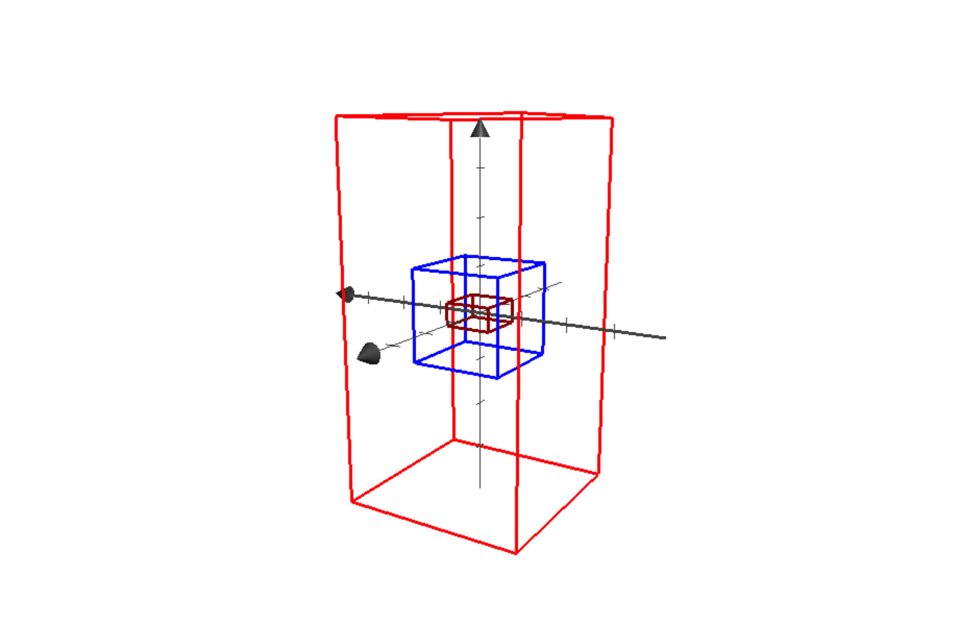 Figure 1
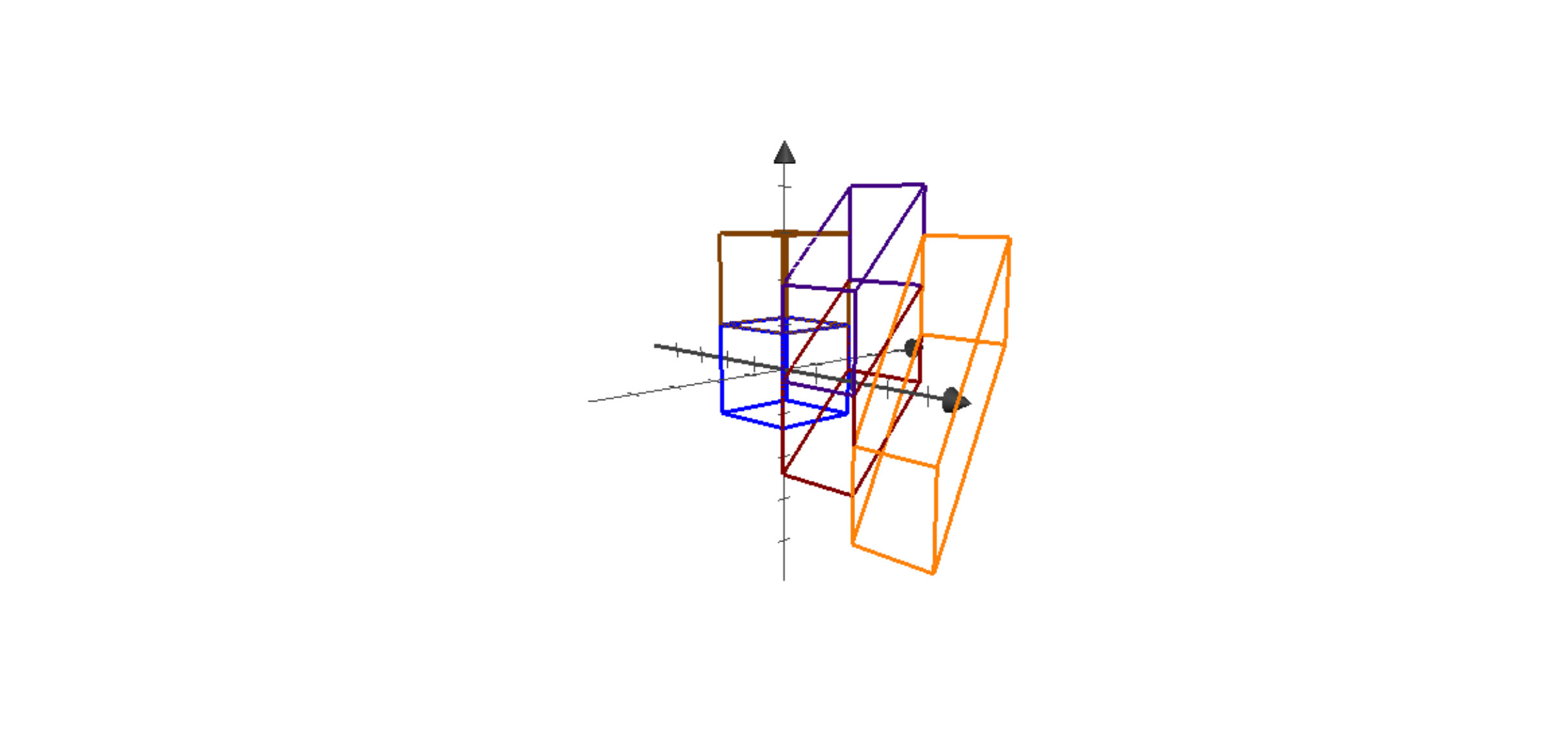 Figure 2
Peer Reviews
No public reviews on file for this paper yet. If you reviewed it on a platform where reviews are public (OpenReview, ICLR, NeurIPS, ICML), you can paste yours below so the community can read it here.
Videos
No videos yet. Explain this paper in a talk, walkthrough, or lecture? Add one.
Taxonomy
TopicsAdvanced Mathematical Modeling in Engineering · Composite Material Mechanics
- convergence and homogenisation for a class of degenerate functionals.
Nicolas Dirr Cardiff School of Mathematics, Cardiff University, Cardiff, UK, e-mail: [email protected].
Federica Dragoni Cardiff School of Mathematics, Cardiff University, Cardiff, UK, e-mail: [email protected].
Paola Mannucci Dipartimento di Matematica “Tullio Levi-Civita” , Università di Padova, Padova, Italy, e-mail: [email protected]
Claudio Marchi Dipartimento di Ingegneria dell’Informazione, Università di Padova, Padova, Italy, e-mail: [email protected]
Abstract
This paper is on -convergence for degenerate integral functionals related to homogenisation problems in the Heisenberg group. Here both the rescaling and the notion of invariance or periodicity are chosen in a way motivated by the geometry of the Heisenberg group. Without using special geometric features, these functionals would be neither coercive nor periodic, so classic results do not apply. All the results apply to the more general case of Carnot groups.
Keywords: Gamma-convergence, homogenisation, Carnot groups, Heisenberg group, Hörmander condition, degenerate functionals.
1 Introduction
-convergence is a notion of convergence of a family of functionals to a functional which goes back to E. de Giorgi (see [16, 17, 18]) and guarantees the convergence of minimisers of the functionals to minimisers of the limit (or effective) functional ; for a precise definition and properties see Section 4.The convergence of minimisers implies, under suitable conditions, convergence of solutions of the Euler-Lagrange equations, and is therefore a useful tool for homogenisation problems, in particular in the random and nonlinear case, see e.g. [14]. If the functional is integral, i.e. of the form
[TABLE]
where is a (Borel) domain, is the distributional gradient of the real-valued function assumed to be in a suitable -space, and with some regularity and growth assumptions, then the corresponding Euler-Lagrange equation is a nonlinear divergence form equation.
The above functional can be generalised to degenerate functionals in the setting of Carnot groups. In this paper we focus specifically on the -dimensional Heisenberg group , which is a step 2 Carnot group defined on (see Section 2 for definitions and properties). Thus the family of functionals considered here is of the form
[TABLE]
where is a domain on while is the horizontal gradient in the Heisenberg group which belongs to a suitable -dimensional subspace of the “space of derivatives” (tangent space), see Definition 2.7. Since , we have : as a consequence, such functionals are typically not coercive in the classical sense, so classical results do not apply.
Working in the setting of the Heisenberg group, the scaling needs to adapt to the underlying geometrical structure, therefore we will consider the following anisotropic scaling with . Hence the scaling is anisotropic w.r.t. the last component. The anisotropy can be understood heuristically in another way: at each point, some directions are “forbidden”, i.e. paths of the associated control problem can move only on a -dimensional subspace of a -dimensional space. By varying their direction often (i.e. by the use of non-trivial commutators from the Hörmander condition) they are able to reach any given point but the cost for “zig-zagging” to get in the forbidden direction is higher, so typically they move slower in these directions, which makes a faster rescaling necessary.
The limit functional is of the same form, i.e.
[TABLE]
where the integral function does not depend on anymore (however the horizontal gradient still depends on trough the vector fields). The corresponding Euler-Lagrange equation will not be elliptic but only subelliptic, we refer to [8, 21] for an overview on subelliptic equations.
The study of homogenisation in subelliptic settings started with the periodic case (see e.g. [4, 7, 23, 24, 6, 29, 34]). The first result for the stochastic case in this degenerate setting is [20], where the authors studied the case Hamilton-Jacobi (first order) case for Hamiltonian depending on the horizontal gradient in the case of Carnot groups.
As -convergence has nice compactness results, the main difficulty is in general the identification of the -limit as again an integral functional. Here it is used that the integrand can be retrieved by considering minimisation problems over small cubes with *affine * boundary conditions, see [12]. A generalisation to the setting of the Heisenberg group requires a suitable adaption of the notion of “affine”, namely -affine functions, see Section 3 for the definition and references. Recently some results for -convergence of degenerate functionals in very general geometries have been proved in [28]. Here we use that the minimal normalised energy on anisotropicaly (Heisenberg dilations) scaled cubes is subadditive by constructing admissible functionals on large cubes and patching together translated minimisers on translated cubes. Here we need to use the specific properties of translations in the Heisenberg group. Note that cubes rescaled by an integer (i.e. ) cannot be written as union of translations of the original cube Q, not even up to a set of measure zero. This a crucial difference with the Euclidean case but we overcome the issue by controlling the error term.
A closely related approach can be found in [25], where the -convergence in Cheeger-Sobolev spaces is considered. Our functional depending only on instead of would be a functional on a Cheeger-Sobolev space, but the natural tiling generalising periodicity in our case does not satisfy the assumptions of [25].
All the results are written in the Heisenberg group for sake of simplicity but the proofs apply to general Carnot groups.
These results can be applied to functionals related to subelliptic -Laplace equations and generalised to stochastic functionals with short correlations (as done in Dal Maso-Modica [13]).
This paper is organised as follows.
In Section 2 we give an overview on the Heisenberg group and its geometry, in particular the scaling, the horizontal gradient and the notion of periodicity.
In Section 3 we define precisely our functionals and we recall the Sobolev spaces adapted to the structure of the Heisenberg group, in particular their embedding into -spaces, through the embedding in fractional Sobolev spaces, which will be crucial for the later -convergence results.
Section 4 is devoted to the -convergence results. We first recall the definition and some basic properties of -convergence. We use compactness properties of the -convergence and we give conditions under which the -limit is again an integral functional, thus recovering the results by Dal Maso-Modica, [12], for our degenerate functionals.
In Section 5 we prove the main result of the paper, that is the homogenisation result for Heisenberg-periodic functionals. In fact, we show a Akcoglu-Krengel type result, [1], for our anisotropic Heisenberg-periodic functionals, i.e. the convergence of normalised minimal energies over rescaled cubes. For this purpose, we exploit an underlying subadditive structure.
In Section 6 we mention some applications and further directions of research. We highlight how the results apply to more general functionals associated to Carnot group structures. We then give some connections with homogenisation for subelliptic -Laplacian. Finally we explain how our methods can be used to generalise the results to the stochastic case with short correlations.
2 Preliminaries: The Heisenberg group.
Carnot groups are non-commutative Lie groups: thus they are endowed both with a non-commutative algebraic structure and with a manifold structure. The lack of commutativity in the algebraic structure reflects on the manifold structure as restrictions on the admissible motions. This means that the allowed curves are constrained to have their velocities in a lower dimensional subspace of the tangent space of the manifold. Then the associated manifold structure is not Riemannian but sub-Riemannian. In this paper we give details for the Heisenberg group only but the results can be easily generalised to Carnot groups (see Section 6). We refer the reader to [8] for definitions and properties on Carnot groups and to [30] for an overview on sub-Riemannian manifolds.
To keep the paper easily readable we omit the intrinsic definition of the Heisenberg group, introducing it directly as the following non-commutative group structure on .
Definition 2.1**.**
The -dimensional Heisenberg group , with , is a Carnot group of step 2 isomorphic to , where , endowed with the following non-commutative group operation:
[TABLE]
for all and where by we indicate the standard inner product in .
In all Carnot groups it is possible to define a natural scaling, induced by the Lie algebra stratification, namely dilations. The dilations replace the multiplication by scalars in the standard vector space structure of the Euclidean .
Definition 2.2**.**
The dilations in the Heisenberg group are the family of group homeomorphisms defined as, for all , with
[TABLE]
Thus the dilations in coincide with the standard Euclidean scaling in the first components while the last component scales as .
The following properties of dilations are true in all Carnot groups and they can be easily checked in the Heiseberg group by using formulas (2.1) and (2.2).
Lemma 2.1**.**
For all , the following properties hold true:
- (1)
; 2. (2)
; 3. (3)
; 4. (4)
for every one has .
We now recall the notion of homogenous dimension. In a general Carnot group , the homogenous dimension is the natural number , where is the step of the stratified associated Lie algebra (see e.g. [8] for more details). In one can easily show that
[TABLE]
The homogeneous dimension is correlated to the scaling of measures since it coincides with the Hausdorff dimension w.r.t. every homogeneous metric. In the paper we always indicate simply by the -dimensional Lebesgue measure of the Borel set of . Then for all , while one can easily show that
[TABLE]
Since the Heisenberg group (as all Carnot groups) is non-abelian, translations to the right or to the left determine two different families of homeomorphism on the group. As standard in this setting, we consider the left-translations, which are defined, for all as with
[TABLE]
where is the group operation defined in (2.1).
Using the left-translations it is possible to define a sub-Riemannian structure on each Carnot group by introducing a suitable family of left-invariant vector fields spanning to the first layer of the Lie algebra stratification. We omit the general definition on Carnot groups (see e.g. [8]). In the specific case of the Heisenberg group, the vector fields can be found as
[TABLE]
where are the unit vectors of the standard Euclidean basis on for . One can also easily show that, for all
[TABLE]
where \big{[}\cdot,\cdot\big{]} are the standard Lie brackets (called also commutators) defined for vector fields. In the case the vector fields are
[TABLE]
We recall that the previous vector fields are left-invariant by definition. For later use we introduce the following simplified notation: given any function , the translation of the function is simply , i.e.
[TABLE]
Thus is a left-invariant vector field if for all and for all fixed
[TABLE]
(while this is in general false considering instead the right-translations).
We recall that the vector fields for span a bracket generating distribution with step 2 (see e.g. [30] for some details).
The previous vector fields allow us to define derivatives of any order, just considering how a vector field acts on smooth functions. Given a function , we denote the horizontal gradient of by
[TABLE]
In the case of the horizontal gradient can be explicitly written as
[TABLE]
We now recall that a differential operator on a the Heisenberg group is called homogeneous of degree if for every one has
[TABLE]
where the scaled function is defined as , for all .
Then we have the following result.
Lemma 2.2**.**
For every , each left-invariant vector field , defined in (2.4), is homogeneous of degree , i.e., for any one has
[TABLE]
The proof is a very simple computation in the Heisenberg group while for general Carnot groups the reader can find a proof e.g. in [22].
This in particular implies that the horizontal gradient is homogeneous of degree one with respect to the dilations , i.e., for every we have
[TABLE]
For later use, it is very useful to introduce the -matrix associated to the vector fields, that is
[TABLE]
where are the left-invariant vector fields defined in (2.4) and the extended matrix of vector fields, which is the -matrix
[TABLE]
where , and is the unit vector spanning the -direction (and associated to the second layer of the stratification for the Lie algebra).
Example 2.1**.**
In the 1-dimensional Heisenberg group , the matrix is the -matrix given by
[TABLE]
while is the -matrix given by
[TABLE]
A trivial computation shows the following property, which will be very useful later: given the quadratic matrix defined in (2.10), then
[TABLE]
The property above means that the left-translations are an isometry for the associated -spaces, i.e. informally setting for all fixed , we have .
Remark 2.1**.**
Property (2.11) can be generalised to all Carnot groups in exponential coordinates or to more general Carnot-type groups (see e.g. [2] for properties and definitions of Carnot-type groups).
Remark 2.2**.**
Trivially where denotes the standard (Euclidean) gradient of .
2.1 Periodicity in the Heisenberg group.
Being the Heisenberg group a Lie group, a very natural notion of periodicity can be introduced by left-translations, see [4, 7, 23, 24]. We refer also to the Phd thesis [26] where periodicity in the Heisenberg group (but also in more general structures as Grushin spaces) is studied in details with many properties and examples. Given any , we say that is H-periodic with period , whenever for all .
For later use in the paper we fix the period . In fact, recalling that , the composition of two left-translations with period is not anymore a integer left-translation since , because the third component becomes , which is in general not anymore an integer.
Instead the composition of two left-translations with period 2 is still a translation of the same type since, for all ,
with . (Note that since the third component is different by a factor in the mixed term.) One could very simply adapt everything to period by choosing a different representation of the Heisenberg group, where the group law is expressed by polynomials with integer coefficients; in that case the unit cell needs to be rescaled to a unit cube (e.g. ), see e.g. [23].
We introduce the following simplified notation for the left-translations with period 2, that is
[TABLE]
We recall that, for all , the following properties hold true:
[TABLE]
A definition of periodicity adapted to the Heisenberg group structure can be given for functions as follows.
Definition 2.3**.**
We say that the function is -periodic whenever
[TABLE]
To construct a large class of periodic functions we need to introduce a H-periodic tiling of . Thus we consider the semiopen cube . We call unit cell and consider . Then one can easily show that the family \big{\{}\tau_{k}(Q)\big{\}}_{k\in\mathbb{Z}^{N}} fullfills
[TABLE]
see Figure 1 and [24, Lemma 2.4].
We next want to highlight a few facts about the scaling of tilings since this will be crucial later when we will study our homogenisation problem. First recall that, in the Heisenberg group, if we scale the unit cell, then we do not get anymore hypercubes but hyper-rectangles since the scaling is anisotropic. In Figure 2 we show how the cube scales for and for . Then if we want to build a tiling of starting by a rescaled cell, we need to be very careful and adapt the translations to the Heisenberg scaling.
Lemma 2.3**.**
Given the unit cell and a , the scaled unit cell as
[TABLE]
then the family \big{\{}Q^{t}_{k}\big{\}}_{k\in\mathbb{Z}^{N}} is a tiling of in the sense that
[TABLE]
- *Proof. * The result follows easily from the properties for and from the fact that
3 A class of degenerate functionals.
Affine functions can be introduced in different ways in the Heisenberg group setting and they have been studied in [15, 3]. For the purpose of the paper, we say that a function is -affine (in the Heisenberg group) if
[TABLE]
for and for some and , where is the projection on the first components and is the standard inner product on . The following lemma is an immediate property of -affine functions in all Carnot-type groups and it will be key for our later results.
Lemma 3.1**.**
For all fixed , we have
[TABLE]
for some and for all .
- *Proof. * One implication (from the right to the left) follows trivially from the fact that does not depend on the last coordinate and the structure of the horizontal gradient.
The other implication follows from the fact that means constant for all , then
[TABLE]
where we indicate by the partial derivative of w.r.t. the variable , for . Using , for all , implies for all , which gives for some .
We will later often use the following notation for H-linear functions:
[TABLE]
We next recall that the definition of Sobolev spaces in the setting of Hörmander vector fields, which applies in particular to the Heisenberg group. We refer to [32, 36]
for more details on these spaces.
Let be an integer, and a domain on . We define the space
[TABLE]
where for . Endowed with the norm
[TABLE]
is a Banach space, and is an Hilbert space in the case .
Moreover, for any , the embeddings
[TABLE]
hold true, where is the step of the stratified associated Lie algebra, thus in Heisenberg group (see e.g. [35]). Later we will also need the following compact embedding.
Lemma 3.2**.**
* is compactly embedded into .*
- *Proof. * This follows from the previous embedding and the fact that the fractional Sobolev space is compactly embedded into (see e.g. [19]).
Definition 3.1**.**
For each domain , we indicate by
[TABLE]
the closure of w.r.t. the Sobolev norm .
This means that, whenever the boundary is regular enough, the trace of vanishes on the boundary of the set.
We will use this notation to express the Dirichlet boundary conditions: more precisely
[TABLE]
are all the functions which coincide on (in the sense of Sobolev space) with some .
Next we recall the following Poincaré inequality, which is key for later results.
Lemma 3.3**.**
Given a bounded domain , then there exists a constant such that
[TABLE]
Consider now a function with and , we introduce the integral functional defined, for all domain , as
[TABLE]
We introduce the following properties for the integrand function
(with and )
[TABLE]
[TABLE]
Moreover for the later homogenisation problem we will assume -periodicity for the functional in the sense of Definition 2.3; more precisely
[TABLE]
Example 3.1**.**
The main example is , which trivially satisfies (3.3) and (3.4) whenever is bounded (with a strictly positive lower bound) and measurable, while assumption (3.5) is equivalent to requiring that is H-periodic.
We want to study the minimisation problem for with -affine boundary condition, i.e.
[TABLE]
with for some and .
Remark 3.1**.**
Note that under assumptions (3.3) and (3.4), the infimum of on the set of functions such that is indeed a minimum by standard arguments, using the convexity, the embedding in Lemma 3.2 and the Poincaré inequality (see Lemma 3.3).
4 A -convergence result for degenerate functionals.
To keep the paper self contained we next recall briefly the definition of -convergence.
4.1 Very brief introduction to -convergence.
In homogenisation theory, we consider a family of solutions to equations with rapidly oscillating coefficients and investigate if they converge to a solution of a homogenised equation with slowly oscillating or constant coefficients. If these equations are the Euler-Lagrange equations of a suitable family of functionals with rapidly oscillating coefficients, and if both minimisers and solutions of the Euler-Lagrange equation are unique, then we can study convergence of the family of functionals instead.
We need a notion of convergence of functionals which guarantees that minimisers of the approximating functionals converge to minimisers of the limit functional.
A suitable mathematical setup to make this rigorous is the notion of -convergence. Let us briefly recall the definition of -convergence (see [9, 10, 11] for more details on this subject).
Definition 4.1**.**
Let be a metric space and for let be a family of functionals on . We say that -converge to if the following conditions are verified:
*for all and for all , there holds *
(-liminf inequality);** 2. 2.
*for all there exist , such that *
(-limsup inequality).**
The convergence of minimisers to minimisers is formalised in the following way, which can be easily derived from Definition 4.1.
Proposition 4.1**.**
If -converge to in , also the corresponding minimal values (or infima) converge. Moreover, if is a minimiser of and , then is a minimiser of .
Hence, the asymptotic behaviour of minimisers of (and therefore solutions of the Euler-Lagrange equations, see Section 6) can be partly understood by considering the -limit of .
Moreover, -convergence has nice compactness properties, i.e. in general it is easy to show that a -limit along subsequences exists. The problem is then to identify this limit (see Section 5) and to show properties of this limit, in particular that it is again an integral functional.
4.2 -convergence limit.
We say that a family of open subsets of with Lipschitz boundary is a substantial family (around ) as if, for every positive , there hold
[TABLE]
where is a constant independent of (see the monograph [33, Ch.8] for other properties).
The following result states that the integral function can be obtained from the minima of the Dirichlet problem for with affine boundary data. To this purpose, for any domain with Lipschitz boundary and for every -affine data, we introduce the following regularised variational problem
[TABLE]
Since the functional depends on only through its horizontal gradient, therefore the constant in the definition of -affine function does not affect the results; we now consider directly the -linear functions defined in (3.1) as boundary data. We state now a useful property, key for the later results.
Lemma 4.1**.**
Let be a -dimensional domain with Lipschitz boundary. For and , and for every smooth function such that on , we have
[TABLE]
- *Proof. * We write . First we show that
[TABLE]
where is the horizontal normal, i.e. with matrix of the vector fields defined in (2.9) and the outward unit normal to , while is the Hausdorff measure defined on . To prove the claim (4.3) we use that the vector fields in the Heisenberg group are divergence free and we combine a simply integration by parts with Remark 2.2, which gives
[TABLE]
where is the -component of for .
Then we can use the divergence theorem again (together with the fact that the vector fields in Carnot groups are divergence free) to conclude:
[TABLE]
for all .
We now use the previous lemma to show that, whenever the integrand function does not depend on , then -affine functions are minimisers for problem (3.6) with -affine boundary condition.
Lemma 4.2**.**
Given a domain with Lipschitz boundary , consider the problem (3.6) with for some and , and defined in (3.2) with convex, then
[TABLE]
Now following the arguments of Dal Maso-Modica [12] for the standard non degenerate case, we prove that the integrand function can be retrieved in term of .
Theorem 4.1**.**
Under assumptions (3.3)-(3.4), there exists a measurable subset of with such that
[TABLE]
for every and with -linear as in (3.1), and every substantial family around .
- *Proof. * We will use the same arguments as in [12, Theorem I] for the non-degenerate case. We just sketch the main steps.
Step 1. Let us at the moment assume that there exists some such that does not depend on for . Then by Jensen’s inequality and by Lemma 4.1, we obtain
[TABLE]
for every , , and defined by (3.1). Exactly as in [12, Proposition 1.1], we can deduce
[TABLE]
It remains to prove that there exists a measurable subset of with such that
[TABLE]
for every and every substantial family around , where
[TABLE]
We observe that for every with and that, arguing as in [12] (recall that is convex w.r.t. ), there exists a positive constant such that: for every and .
Fix a dense subset of . The Lebesgue’s Differentiation Theorem ensures that there exists a measurable subset of with such that
[TABLE]
for every substantial family around . Moreover, as in [12], for every , there exists a finite set such that
[TABLE]
Therefore, we infer
[TABLE]
for every substantial family around . By the arbitrariness of , we accomplish the proof.
Step 2. Let us now remove the additional assumption of Step . Taking into account the convexity and the coercivity of w.r.t. , by the same arguments as in [12, Theorem I], we obtain that there exists a measurable set , with , such that
[TABLE]
for every family as in the statement. In order to obtain the reverse inequality, we first observe that the same arguments of [12, Lemma 1.2] ensure that there exists an increasing sequence of functions such that and each satisfies the assumptions of step . For each , we denote and respectively the corresponding functional and the negligible set given by step . We set . Step for and the inequality entail
[TABLE]
for every family as in the statement. Passing to the limit as , one deduces
[TABLE]
for every family as in the statement. Finally, we accomplish the proof by choosing .
We denote by the set of all functional which satisfy assumptions (3.3)-(3.4) with the same constants , and . In the next result, we obtain a characterization of -convergence in terms of the convergence of the minima of problems with Dirichlet boundary conditions. We like also to mention that very recently some results in this direction have been proved in [28] in much more general geometries but with quite different techniques.
Theorem 4.2**.**
Let be a sequence of functionals in . Let be a dense subset of . Let be a family of open bounded subsets of which contains a substantial family around every point . Assume that for each and for each there exists . Then, there exists a functional such that the sequence -converge to and
[TABLE]
for every and for every bounded domain of with Lipschitz boundary.
- *Proof. * The proof follows exactly the same arguments of the proof of [12, Theorem IV] so we just sketch the main issues. We first claim that the space can be endowed with a metric such that is a compact metric space and a sequence of functionals in is convergent w.r.t. to to some if and only if it -converges to . Indeed, this property can be obtained following the same arguments of [13, Proposition 1.21] and taking advantage of the properties of and of for the Heisenberg group, in particular the Rellich compact injection and the Poincaré inequality respectively in Lemma 3.2 and in Lemma 3.3. Hence, we shall omit it.
Even if the rest of the proof follows the arguments in [12], for the sake of completeness, let us recall the role of Theorem 4.1. Let and two subsequences of which -converge respectively to some and to some . We claim: . Actually, we have
[TABLE]
Theorem 4.1 ensures that there exists a measurable set , with , such that
[TABLE]
where and are the integrands of and respectively of . Finally, the convexity of and of permits to extend the previous equality to every .
5 Periodic homogenisation for degenerate functionals with -affine data.
Given the functional defined in (3.2), we now introduce for all the following rescaled functionals:
[TABLE]
and for all , the following translated functionals:
[TABLE]
Following the idea in [14], for all fixed , for all bounded domain , and with and , we introduce the following notation
[TABLE]
where we recall that is a -affine boundary data.
We next define
[TABLE]
Lemma 5.1**.**
Given a bounded domain of , there holds
[TABLE]
- *Proof. * Note that since the functional depends only on the gradient of the function, . Thus to prove (5.4) is the same of proving
[TABLE]
In order to prove (5.5) we start looking at the right-hand side and defining . Since and differ only by a constant, obviously
[TABLE]
where we recall that by definition of translated function.
Now we consider the following change of variables (equivalently where is the inverse element w.r.t. the group law ).
An easy computation shows that the Jacobian of the change of variables is exactly the matrix defined in (2.10). Then property (2.11) tells that . Since are defined as left-invariant vector fields for all (see (2.6)) we also know that
[TABLE]
Moreover if and only if and
[TABLE]
where : in fact on we have . Then in the new variables we have
[TABLE]
To conclude we now define . Using again the property of left-invariant vector fields, we have then
[TABLE]
The chains of identities in (5.6), (5.7) and (5.8) give identity (5.5) and conclude the proof.
The following result is an immediate consequence of the previous lemma in the case of -periodic functionals.
Lemma 5.2**.**
Assume (3.5), then, for all bounded domains and for all and
[TABLE]
In the following lemma we show how the assumptions on the integrand are inherited by .
Lemma 5.3**.**
Let be a bounded domain in with Lipschitz boundary, and defined in (5.3) and let be measurable.
- (i)
If satisfies assumption (3.4), we have
[TABLE]
where and are the same constants given in (3.4). 2. (ii)
If satisfies assumption (3.3), we have for all and for all
[TABLE]
- *Proof. * Using that is admissible for the minimum defining and that , we get
[TABLE]
Moreover
[TABLE]
where for the last identity we use Lemma 4.2 for the convex function , which tells that the minimisers are the -affine functions, whenever does not depend on .
It remains to prove (ii). To this end it is enough to remark that for all functions and which are admissible respectively for and , then is admissible for , which implies
[TABLE]
Taking the minimum over all admissible and , we get property (ii).
To prove the convergence of the functional as , we need to show now a sort of Akcoglu-Krengel type result (see [1]) for periodic functionals, adapted to the anisotropic structure of the Heisenberg group. In [25] the authors prove a very interesting Akcoglu-Krengel type result for general metric measure spaces. We need to mention that unfortunately the result therein does not apply to our case. In fact it is quite easy to show that the Heisenberg group endowed with the Carnot-Carathéodory metric (or also with the homogeneous metric) and the Lebesgue measure is a \big{(}G,\{\delta_{t}\}_{t>0}\big{)}-metric measure space where is the subgroup of homeomorphisms on the Heisenberg group defined by the left-translations w.r.t. an element in . Nevertheless one can also show that in general that space is not “meashable” according to the definition introduced in [25]. We give a self-contained proof which can be later adapted to the stochastic case (which will be a topic in a forthcoming paper, see Section 6).
We now recall that, defining for all , , we know that (see (2.3)), where is the homogeneous dimension, then in in particular .
The next lemma tells that, as , we can reduce to take the limits only over integer subsequences.
Lemma 5.4**.**
Assume that the limit exists for integer sequences, i.e. for ,
[TABLE]
Then for all sequences with it holds
[TABLE]
- *Proof. * For we define
[TABLE]
Fix and choose large enough that for
Denote by and which are both finite by Lemma 5.3. We can find such that
[TABLE]
Define (where by we indicate the integer part of a real number) and let be a function with -affine boundary conditions on such that We extend to by letting it equal to the boundary condition on , i.e. given by
[TABLE]
whose restriction to is an admissible function for Note that
[TABLE]
hence
[TABLE]
where the constant depends on and Since is admissible for so we estimate
[TABLE]
Note that
[TABLE]
so, by choosing, if necessary, larger, we can make the right hand side thus, as was arbitrary, we have shown
For the opposite inequality, we use estimates similar to what we did before: we can find infinitely many such that
[TABLE]
Therefore we take and let be a function with -affine boundary condition on such that We extend to a function on which is admissible for and equals on Arguing as before we get
[TABLE]
Then
[TABLE]
By choosing, if necessary, larger, we can make the right hand side smaller than thus we have shown but as we have
We denote the set of natural numbers excluding 0. We next prove an Akcoglu-Krengel type result.
Theorem 5.1**.**
Let consider the (semiopen) unit cell and let and be defined in (5.3). Assume that is measurable and satisfies (3.4) and (3.5), then
[TABLE]
where is the non-negative constant given by
[TABLE]
- *Proof. * Note that, by Lemma 5.3 - (i),
[TABLE]
so in particular .
Step 1. Since is defined as infumum over , trivially \frac{\mu_{q}\big{(}Q^{k}\big{)}}{|Q^{k}|}\geq C_{q} for all , which implies
[TABLE]
Step 2. We next show the limsup estimate. Using the definition of infimum for , for all , and the definition of , then there exists and and such that
[TABLE]
where is the functional defined in (3.2). This sums up as follows
[TABLE]
Recall the definition of given in (2.12); we use such translations to extend to the whole by translating periodically the gradient. More precisely, let us introduce
[TABLE]
Using that , we can define
[TABLE]
where by we indicate the characteristic function of the set ; recall also that . The function is well-defined since are all disjoint. We can easily check that is continuous on : in fact, for , then and, whenever , we have which implies
[TABLE]
which does not anymore depend on . The continuity of on , together with the fact that , imply that U_{\rho}\in W^{1,\alpha}_{\mathcal{X},\textrm{loc}}\big{(}\mathbb{R}^{N}\big{)}.
We next introduce the following two objects:
[TABLE]
and we construct a new function , which is admissible for , as
[TABLE]
By definition v_{\rho}-l_{q}\in W^{1,\alpha}_{\mathcal{X},0}\big{(}Q^{k}\big{)}, and
[TABLE]
First we compute
[TABLE]
where we have used that are disjoint. If , then U_{\rho}(x)=q\cdot\pi_{m}(j_{\rho})+u_{\rho}\big{(}\tau_{-j_{\rho}}(x)\big{)}. By using that the vector fields are left invariant, we get
[TABLE]
Thus, by using the change of variables and recalling that the determinant of the Jacobian is 1 (see (2.11)), we get the following chain of identities:
[TABLE]
where in the last identity above we have used the periodicity assumption on (see assumption (3.5)). The integrals in the last term of (5.12) do not depend anymore on , then
[TABLE]
where the last inequality follows from (5.10).
Put together (5.11),(5.12) and (5.13), we get the following estimate:
[TABLE]
It remains to estimate the integral on the complementary of by using that for all by definition, hence
[TABLE]
Estimates (5.14) and (5.15), together with the fact that is admissible for , give
[TABLE]
where in the last inequality we have used that and |\widehat{S}^{\rho}_{k}|=\textrm{card}\big{(}S^{\rho}_{k}\big{)}|Q^{k_{\rho}}|, which together imply \frac{\textrm{card}\big{(}S^{\rho}_{k}\big{)}\,|Q^{k_{\rho}}|}{|Q^{k}|}\leq 1.
To conclude we claim that the following limit holds true:
[TABLE]
Then, by simply taking the limsup as in the inequality (5.16) and using claim (5.17), we get
[TABLE]
which conclude the proof as .
It remains only now to prove claim (5.17). By a simple rescaling we can actually show that this limit is the same as the one shown in the proof of Lemma 2.21 in [24]. In fact, set , then by using the properties of dilations (Lemma 2.1)
[TABLE]
Set , by using the properties of dilations and left-translations one can easily check that
[TABLE]
Thus by using the limit proved in [24] we conclude the proof.
We define as
[TABLE]
where is the limit proved in Theorem 5.1.
From Lemma 5.3, one can show that keeps the properties of simply by passing to the limit as . More precisely
Lemma 5.5**.**
Given measurable, the following properties hold:
- (i)
if assumption (3.4) is satisfied, then
[TABLE]
where and are the same constants given in (3.4). 2. (ii)
if assumption (3.3) is satisfied, then for all
[TABLE]
We now prove the main result of the paper.
Theorem 5.2**.**
Given a bounded domain with Lipschitz boundary, and the functional defined in (3.2). Let us assume that (3.3), (3.4) and (3.5) hold true, and for some and . Define the rescaled functionals introduced in (5.1) and let us consider the corresponding minimisation problems for (see (3.6)) then
[TABLE]
where the limit functional can be characterised as
[TABLE]
and defined as with constant given in Theorem 5.1.
Moreover the limit function is still measurable, convex and satisfies the same growth condition (3.4) satisfied by .
- *Proof. * Applying Theorem 4.2 we deduce that -converge to some functional . Let us now prove that the limit functional can be identified as the integral functional associated to given in (5.18). Choose as substantial family , and fix , at the moment let us assume the following claim:
[TABLE]
with homogeneous dimension.
By using that all the previous results in Section 5 can be obtained replacing with the cube , we have
[TABLE]
By Theorem 4.1, passing to the limit as , we conclude .
It only remains to check claim (5.19). At this purpose, we use the change of variables ; hence recalling definition (5.3) and using that is the scaled function defined as , we have
[TABLE]
by simply using that and (2.3). Defining the function and using Lemma 2.2, we have that
[TABLE]
Moreover informally we have that, for , . Hence (5.20) gives
[TABLE]
which proves claim (5.19).
The properties for the limit function are proved in Lemma 5.5.
6 Applications and generalizations
We conclude listing further directions in which we are presently working, for some of which we obtained already some partial results.
6.1 Homogenisation for functionals associated to Carnot groups
and the subelliptic -Laplacian.
As mentioned in the introduction all the proofs never use the specific structure of the Heisenberg group but they instead use properties true for all Carnot groups. So all the results apply without any modification to the general case of Carnot groups.
As it is well-known by Euler-Lagrange equations, we can connect minima of functionals to solutions of PDEs. Whenever uniqueness holds this correspondence is one-to-one. Then our results can be used to study homogenisation for several subelliptic PDEs and in particular for the subelliptic -Laplacian, which is defined, for , as
[TABLE]
where is a symmetric matrix satisfying the usual ellipticity condition. Equations of this form have been studies by many authors, see e.g. [31] and references therein. The functional associated to the -Laplacian is
[TABLE]
Note that satisfies all our conditions for all . Then we can apply Theorem 5.2. It remains now to show that the limit functional has still the structure of a functional associated to a subelliptic -Laplacian equation (work in preparation).
6.2 Stochastic functionals.
Another generalisation is the case of random functionals, i.e. integral functionals of the form
[TABLE]
where belongs to a probability space and the integrand is stationary and ergodic with respect to left translations. For a precise definition of stationary ergodic in the setting of Carnot groups we refer to [20], where the authors prove an homogenisation result for stochastic Hamilton-Jacobi equations. The general stationary ergodic case will be treated in a forthcoming paper, but we sketch here a proof for the simpler situation of short correlated random variables.
More precisely, we assume that the random integrand satisfies (3.3) and (3.4) uniformly in and (3.5) in law, i.e. the random integrand and its translations are not equal, but have the same law as random variables. In addition, we require that there exits a constant such that and are independent, if where by we indicate the homogeneous distance in Carnot groups, i.e. for example in 1-dimensional Heisenberg where |x|_{h}:=\big{(}(x_{1}^{2}+x_{2}^{2})^{2}+x_{3}^{2}\big{)}^{1/4}. Note that this is different from being short correlated in the Euclidean distance.
Under these assumptions one can show along the lines of [13] that
[TABLE]
in probability to a constant , and conclude convergence of the functionals in probability to an integral functional with constant integrand
As a first step, defining
[TABLE]
one can show along the lines of Section 5 that
[TABLE]
for some constant . Note that because of the invariance in law, Lemma 5.2 holds for but not for with fixed.
Now fix so large that
[TABLE]
and now fix , we use the construction in step 2 of the proof of Theorem 5.1 to show that
[TABLE]
The r.h.s. is a normalised sum over independent, identically distributed random variables with mean close to By the weak law of large numbers, we have that for and sufficiently large the quantity
[TABLE]
is small. Now define
[TABLE]
We have
[TABLE]
As we can make arbitrarily small by choosing big, this implies that for such also in order to avoid the contradiction
Acknowledgments. The first author was partially supported by EPSRC via grant EP/M028607/1. The third and the fourth author are members of GNAMPA-INdAM and have been partially supported also by the Fondazione CaRiPaRo Project “Nonlinear Partial Differential Equations: Asymptotic Problems and Mean-Field Games”. They warmly thank University of Cardiff for the kind hospitality.
The reference list from the paper itself. Each links out to its DOI / PubMed record.
- 1[1] M.A. Akcoglu, U. Krengel, Ergodic Theorems for Superadditive Processes , J. Reine Angew. Math. 323 (1981), 53-67.
- 2[2] M. Bardi, F. Dragoni, Convexity and semiconvexity along vector fields , Calc. Var. Partial Differential Equations 42 (2011), no. 3-4, 405–427.
- 3[3] M. Bardi, F. Dragoni, Subdifferential and Properties of Convex Functions with respect to Vector Fields , J. Convex Analysis 21 (2014), no. 3, 785–810.
- 4[4] I. Birindelli, J. Wigniolle, Homogenisation of Hamilton-Jacobi equations in the Heisenberg group , Commun. Pure Appl. Anal. 2 (2003), no. 4, 461–479.
- 5[5] M. Biroli, Subelliptic Hamilton-Jacobi equations: the coercive evolution case , Appl. Anal. 92 (2013), no. 1, 1–14.
- 6[6] M. Biroli, C. Picard, N. A. Tchou, Homogenization of the p 𝑝 p -Laplacian associated with the Heisenberg group. Rend. Accad. Naz. Sci. XL Mem. Mat. Appl. 22 (1998), no. 5, 23–42.
- 7[7] M. Biroli, U. Mosco, N.A. Tchou, Homogenisation for degenerate operators with periodical coefficients with respect to the Heisenberg group . C. R. Acad. Sci. Paris Sér. I Math. 322 (1996), no. 5, 439–444.
- 8[8] A. Bonfiglioli, E. Lanconelli, F. Uguzzoni, Stratified Lie Groups and Potential Theory for their Sub-Laplacians , Springer, Berlin, 2007.