On amplitudes, resonances and the ultraviolet completion of gravity
Rodrigo Alonso, Alfredo Urbano

TL;DR
This paper proposes a possible ultraviolet completion of gravity using on-shell methods, predicting an infinite tower of resonances and deviations from General Relativity, with implications for string theory and spacetime structure.
Contribution
It introduces a novel bottom-up approach to gravity's ultraviolet completion using on-shell techniques, incorporating an infinite resonance spectrum and duality relations.
Findings
Predicts an infinite tower of resonances with increasing spin and mass.
Suggests deviations from General Relativity in gravity-fermion couplings.
Links the amplitude structure to string theory-like form factors.
Abstract
This letter constructs, making use of the on-shell spinor-helicity formalism, a possible ultraviolet completion of gravity following a "bottom-up" approach. The assumptions of locality, unitarity and causality i) require an infinite tower of resonances with increasing spin and quantized mass, ii) introduce a duality relation among crossed scattering channels, and iii) dress all gravitational amplitudes in the Standard Model with a form factor that closely resembles either the Veneziano or the Virasoro-Shapiro amplitude in string theory. As a consequence of unitarity, the theory predicts leading order deviations from General Relativity in the coupling of gravity to fermions that could be explained if space-time has torsion in addition to curvature.
Click any figure to enlarge with its caption.
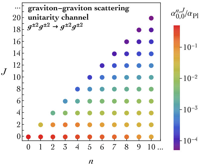 Figure 1
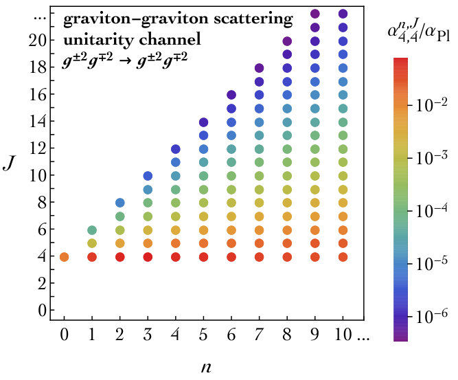 Figure 2
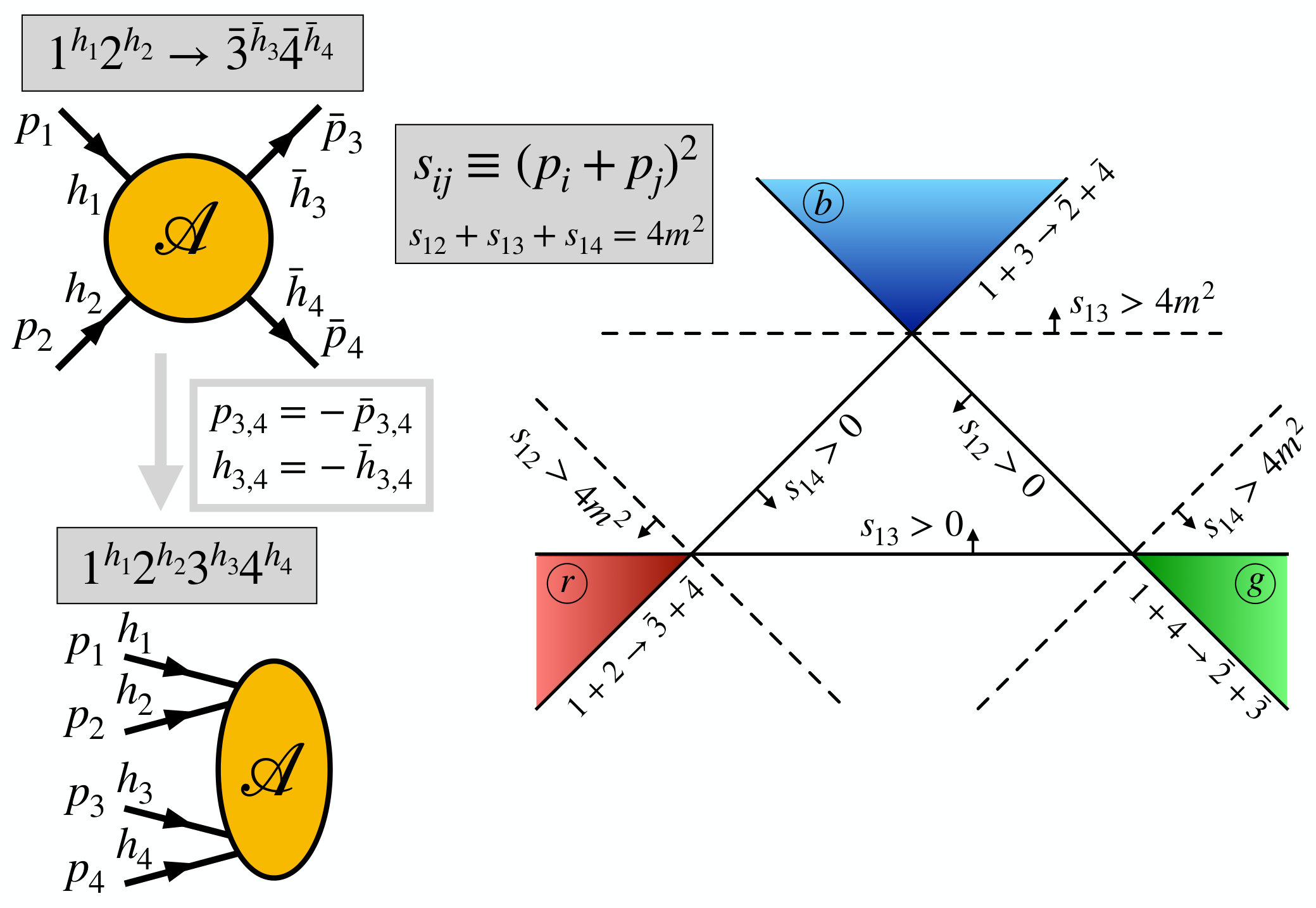 Figure 3
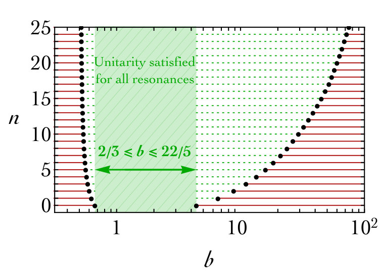 Figure 4
| Scalar | Fermion | Vector | Graviton | |
| Scalar | ||||
| Fermion | ||||
| Vector | ||||
| Graviton | ||||
| N | 1 | 2 | 3 | 4 | 5 | 6 | ||
| ✗ | ||||||||
| ✗ | ✗ | |||||||
| ✗ | ✗ | ✗ | ✗ |
| 1 | 2 | 3 | 4 | 5 | |||
| ✗ | |||||||
| ✗ | |||||||
| ✗ | |||||||
| ✗ |
| N | 1 | 2 | 3 | 4 | 5 | ||
| ✗ | |||||||
| ✗ | |||||||
| ✗ | |||||||
| ✗ |
| 3/2 | 5/2 | 7/2 | 9/2 | 11/2 | |||
| ✗ | |||||||
| ✗ | |||||||
| ✗ | |||||||
| ✗ |
Peer Reviews
No public reviews on file for this paper yet. If you reviewed it on a platform where reviews are public (OpenReview, ICLR, NeurIPS, ICML), you can paste yours below so the community can read it here.
Videos
No videos yet. Explain this paper in a talk, walkthrough, or lecture? Add one.
\usetkzobj
all
IPMU 19-0091
On amplitudes, resonances and the ultraviolet completion of gravity
Rodrigo Alonso
Kavli Institute for the Physics and Mathematics of the Universe (WPI)
University of Tokyo, Kashiwa, Chiba, 277-8583 Japan.
Alfredo Urbano
INFN, sezione di Trieste, SISSA, via Bonomea 265, 34136 Trieste, Italy;
IFPU, Institute for Fundamental Physics of the Universe, Via Beirut 2, 34014 Trieste, Italy.
Abstract
This letter constructs, making use of the on-shell spinor-helicity formalism, a possible ultraviolet completion of gravity following a “bottom-up” approach. The assumptions of locality, unitarity and causality i) require an infinite tower of resonances with increasing spin and quantized mass, ii) introduce a duality relation among crossed scattering channels, and iii) dress all gravitational amplitudes in the Standard Model with a form factor that closely resembles either the Veneziano or the Virasoro-Shapiro amplitude in string theory. As a consequence of unitarity, the theory predicts leading order deviations from General Relativity in the coupling of gravity to fermions that could be explained if space-time has torsion in addition to curvature.
I Introuduction
Prior to the Large Hadron Collider turn on, our tested theory of Nature was a gauge effective field theory (EFT) with a scale at which unitarity was lost perturbatively. Unitarity, however, is sacred and its guardian – as present data seem to indicate – is the Higgs boson. Despite all the apparent differences, the categorization above applies word for word to gravity when thought of as an EFT with scale and diffeomorphisms as gauge transformations, even though as for who its ‘Higgs(es)’ is (are), there is no experimental evidence at present. Exposing the need for a ultraviolet (UV) completion of gravity by means of its similarities with the Standard Model (SM) is preeminently a particle physicist “bottom-up” approach, and it is not to say that this is the sole issue in gravity that needs addressing (open problems range from a non-perturbative formulation to the understanding of singularities relevant in cosmology and astrophysics Woodard (2009)). It is, nonetheless, the point of view that rules the course of this letter.
One can further elaborate that the above formulation, even within particle physics and EFT, is obscured by (of course fundamental) differences in the gauge symmetry, treatment of the massless mediator, the universality of gravity etc. In order to sidestep these differences, the best suited subject of study are on-shell amplitudes; they circumvent gauge redundancies, field redefinitions and gauge fixing present at the Lagrangian level while making ostensible the high-energy behavior. Furthermore, as for practical implications, the derivation of these amplitudes with conventional Feynman rules is greatly involved (the three- and four-graviton vertex derived from the Einstein-Hilbert action have, respectively, about 100 and 2500 terms when fully expanded DeWitt (1967)) to finally collapse in a single-term remarkably simple amplitude Berends and Gastmans (1975); Grisaru et al. (1975); Sannan (1986).
This is part of the evidence that supports postulating a theory with amplitudes as the starting and building blocks. This approach is the on-shell amplitude program, see Dixon (1996); Elvang and Huang (2013); Arkani-Hamed et al. (2017) for reviews. An important part of it is the on-shell spinor-helicity formalism, which seeks to exploit helicity (little group) transformation properties to determine the shape of amplitudes while providing a common framework to formulate scattering amplitudes for all spins and, more recently, all masses Arkani-Hamed et al. (2017). Combined with a recursive method to build higher point amplitudes from lower point ones (BCFW, CSW Cachazo et al. (2004); Britto et al. (2005)), this program aims at a self-contained formulation of quantum field theories. It is not without its own challenges, as determination of off-shell contributions prevents these methods to extend to arbitrary theories.
If one is to sidestep the Lagrangian formulation, however, care should be taken to ensure that the properties that are naturally implemented in it are satisfied by the formulated amplitudes. Since they are of particular importance in this work, let us briefly review them. Locality. Interactions are either point-like or mediated by the exchange of particles propagating between two space-time points. This elementary principle dictates the non-analytic structure of scattering amplitudes: the only singularities occur when one or more intermediate particles go on-shell. Unitarity and Causality. The scattering matrix is a unitary operator as a consequence of probability conservation, and causality implies that local observables must commute outside the light-cone in position space Gell-Mann et al. (1954). Positivity, derived from unitarity, will play a central role in the analysis of this letter. These principles impose, in addition, stringent constraints on the high-energy behavior of scattering amplitudes Adams et al. (2006); of relevance in this work will be the extension of the Froissart bound Froissart (1961) to a theory with a massless graviton Camanho et al. (2016) in the forward limit and the Cerulus-Martin bound Cerulus and Martin (1964); Epstein and Martin (2019) in the hard scattering region. Furthermore, the property of causality results in analyticity of the scattering amplitude thus making possible to represent the latter by means of a dispersion relation via Cauchy’s theorem Gribov (2012).
In line with the “bottom-up” perspective mentioned above, we shall explore in this work whether it is possible to obtain a UV completion of gravity by adding massive resonances, and, if so, what are the properties required of them. To this end, we shall combine the on-shell spinor-helicity formalism with the above-mentioned fundamental properties. In addition, the discussion will be restricted to weak coupling and tree level, which is to say in typical EFT language that the new resonances should lay below .
II Amplitudes for Gravity
In this section we construct the elementary components of this study, these are three- and four-point amplitudes mediated by gravitational and massive spin resonance interactions (section II.1 and II.2, respectively). It will also serve as introduction to the formalism for the unacquainted reader.
II.1 Graviton mediated amplitudes
On-shell Dirac or Weyl spinors, polarization vectors and polarization tensors are objects that interpolate between the Lorentz group and the little group – that is for massless or for massive particles – and, as such, transform under representations of both. The on-shell spinor-helicity formalism in essence seeks to use group theory in both groups to determine the shape of amplitudes. The simplest case is that of massless fermions; denote as () an on-shell momentum left-handed (right-handed) spinor with () index () and anti-symmetric metric (), . The spinor () represents a helicity () particle and hence transforms under as . Amplitudes are Lorentz invariant quantities but they comprise little group representations, and so a valid amplitude for two left-handed fermions is . The massive case is obtained upgrading the spinor to the fundamental representation with an index which again has anti-symmetric metric . Here we will typically omit the index but use boldface to separate it from the massless case following Arkani-Hamed et al. (2017). The reader accustomed to Dirac spinors will find these variables demystified by the relation in Weyl’s basis for .
One has then that higher spin is simply built out of the fundamental representations; the familiar polarization vectors read, e.g. with an auxiliary spinor and with the Pauli matrices. Objects like polarization vectors or tensors, however, will not appear in the formalism since one rather starts from amplitudes and demands proper little group scaling; for instance an amplitude describing a particle with momentum and helicity , , scales as . As conventional in amplitude methods we will derive amplitudes with all particles coming in, and we summarize our conventions about kinematics in fig. 1. Given the scattering of particles 1,2 with momenta and helicities into particles with momenta and helicities , denoted here , the all-incoming amplitude, , is obtained changing the sign of the momenta (and with it the helicities) of the outgoing particles , . Equivalently starting from an all incoming amplitude and taking some of the legs out going, will turn into one of the three Mandelstam variables as given in fig. 1 whereas an incoming left-handed spinor will turn into representing an outgoing momentum helicity +1/2 particle (our convention for the phase is in appendix A). Here we find it useful to write amplitudes in terms of since they make clear the connection between different physical processes related by crossing transformations, symmetries under particle exchange (eg. ) and can be viewed as a function with support on 3 different disconnected regions (r), (b), (g) as shown in fig. 1. Finally, for energies close to the approximation of massless matter (i.e. SM particles), which we shall adopt in the following, is excellent.
The first step in our quest for the “bottom-up” UV completion of gravity with amplitude methods is to build the on-shell three-point amplitudes describing interactions of SM particles with gravity by means of Lorentz-invariant combinations of appropriate powers of spinor variables. As stated in the introduction, we restrict to tree-level amplitudes, and our theory of gravity is General Relativity (GR). A graviton of helicity and momentum coupling to a particle of momentum , helicity and a particle of helicity reads by little group scaling:
[TABLE]
with the same and opposite sign yielding, respectively, mass-dimension of or , and where the short-hand notation etc. is implied. Given that an -point amplitude has mass-dimension and gravity’s coupling is with mass-dimension , we find that only one of the two amplitudes is generated. Explicitly
[TABLE]
This on-shell amplitude has and is gauge invariant, as can be checked by shifting and projecting in terms of the spinors. The absence of a amplitude means that gravity conserves helicity which at this level coincides with any quantum number that the particle might have. As we shall see in the rest of our analysis, this observation plays an important role.
The four-point amplitude of order is generated by graviton exchange, and hence contains a pole. The residue of this pole factorizes into the product of two local three-point on-shell amplitudes, given above. One can, therefore, reconstruct the on-shell part of the four-point amplitude as
[TABLE]
where given that the helicity graviton with momentum enters the second vertex with momentum and helicity . Two currents of possibly different helicity with are considered for arbitrary SM external states. Manipulation of the expression above leads, using the on-shell conditions, to (for brevity let us denote )
[TABLE]
where is an integer for integer or semi-integer is so is , and , . The appearance of this parameter is related to the extension of the amplitude off-shell; whereas the dependence on spinor variables is fully fixed by the little group, one has that on-shell (i.e. when ) , and so amplitude methods alone cannot determine .111Locality bounds to range in the interval in order to avoid double poles. This is because we have the scaling , , and the condition above ensures that no negative powers of are present. From the scaling with energy of the energy-momentum tensor, we find . Furthermore when a scalar current is present () gravity has no handle to distinguish between particles and , and the amplitude must be symmetric. The ambiguity in , therefore, reduces to two cases only, each characterized by one parameter , as displayed explicitly in table 1.222Knowledge of the full amplitude in GR can be attained through a Feynman rule computation. Here however we keep the contact terms arbitrary. In this sense, note that experimentally we have only tested the pole terms, i.e. the long range interaction In this table we collect all tree-level SM scattering amplitudes mediated by gravity constructed explicitly by means of eq. (10). We also display gravitational Compton scattering (i.e. scattering among gravitons and SM particles) and graviton-graviton scattering. These cases have their helicity structure dictated by the same formula of eq. (10) but now there are poles in all three Mandelstam variables and we find the denominator (i.e. ).
What is more, one has that the formula in eq. (10), comprises all tree-level four-point amplitudes generated in GR. The amplitudes can be split into matter-matter, matter-graviton and graviton-graviton scattering (here and in the following ‘matter’ generically refers to scalars, fermions and vectors). The fact that gravity does not change the helicity of matter implies that the amplitudes in table 1 are the only non-vanishing matter-matter cases, one can see this diagrammatically and derive the helicity conservation rule . This is not clear, however, for scattering with gravity where the three point vertex with structure
[TABLE]
produces a diagram in which the helicity is exchanged thus leading to a situation where . The result of summing all diagrams, however, yields a vanishing amplitude in this case (not only for the pole terms but the full amplitude as can be obtained with Feynman diagrams). The same occurs for graviton scattering which makes table 1 complete at tree level.
II.2 Massive spin J mediated amplitudes
Consider now the exchange of a massive spin resonance. Massive spinning particles in the spinor-helicity formalism are represented by symmetric tensors on the spinor variables, i.e. for a particle with momentum , . The coupling of this spin resonance with mass to (massless) matter with helicities is given by the following three-point amplitude, completely determined by little group scaling
[TABLE]
where we introduced the coupling constant , omitted Lorentz indexes, and we note that, to avoid inverse powers of , since otherwise we would get a vanishing amplitude. We now move to construct on-shell four-point amplitudes, and we divide our analysis in three steps.
II.2.1 Legendre polynomials
In order to isolate the differences with massive mediators and for exposition purposes we consider first the case with external scalar particles. For a conventional diagrammatic derivation of the following results see, e.g. Francia et al. (2007); Caron-Huot et al. (2017). A simple manipulation of eq. (12) in this case brings the spinor structure into the form
[TABLE]
where we use matrix notation to omit Lorentz indices. We next construct the amplitude contribution from the on-shell exchange of the massive particle, which decomposes into
[TABLE]
The complication lies in performing the sum over spinor -indexes. An example of such a configuration can be depicted as (the minus sign in () can be pulled out of the spinors to contribute a factor)
[TABLE]
Where the solid green lines signal the summed little group indexes while the dotted follows the matrix multiplication in Lorentz indexes. Using the completion relations and we can reduce any of the above terms to a product of traces333Implicit in our notation for products of ’s is the proper contraction of Lorentz indices, = with over slashed momenta as with and an ordered array. For instance with one such configuration is and its coefficient is given by counting the ways to accommodate a single lasso ‘o’ and double one ‘’ in 3 slots; oo, etc; examples for are given in the appendix, eqs. (149, 150, 151). In a second step we collapse the traces into polynomials in , , using the relation in eq. (152) in the appendix.
All in all we get the following expression for the four-point amplitude
[TABLE]
where are Legendre polynomials and
[TABLE]
where we have used the on-shell condition in and .
We consider next the case with equal helicity in the three-point amplitude. The spinor structure takes the form
[TABLE]
This is the same structure we already found in the scalar case, eq. (13). This means that in the computation of the four-point amplitude the case with equal helicity reduces to the previous result in eq. (14) with Legendre polynomials, with an overall factor that takes into account the helicity of the external particles. As an important difference, however, notice that in this type of coupling the interaction with the massive spin resonance changes any quantum number that matter might have.
II.2.2 Jacobi polynomials
Consider now the case with opposite helicity which corresponds to a helicity and quantum number conserving interaction as is the case for the graviton coupling. The dependence on spinor variables reads
[TABLE]
The derivation of the four-point amplitude in this case is not a mere rescaling of the scalar case but one can follow the same steps in the computation,
[TABLE]
with . As in the computation that lead to eq. (14) one can use the completion relations for the sum in little group indices of , to obtain traces over indices. The computational difference is that traces are not just over chains of and but factors of and might replace each one of the two factors, e.g. in tr. The number of possible traces grows much steeply now so instead one can take a faster approach building on the scalar result. Take eq. (14) with ’s contracted with ’s as obtained after working out combinatorics and expanding traces in Lorentz scalar products of momenta. Then one can substitute to get the result for polarized states (note that longitudinal pieces drop out, ). This means that we need to unfold the sum in eq. (14) to insert factors of and of ; this is again a combinatorics problem that results in, denoting
[TABLE]
with as in eq. (15) and as
[TABLE]
where the sum runs over values of with non-negative-entry binomials. Although written in an unusual form, we find that the polynomial in
[TABLE]
is proportional to the Jacobi polynomials
[TABLE]
All in all, eq. (II.2.2) reads
[TABLE]
and it does contain the scalar and the same helicity cases as the Jacobi polynomials reduce to Legendre polynomials in both limits. Let us also note that the measure for Jacobi polynomials is , in our case , and it is related to the helicity scaling of the amplitude as we shall see next. The appearance of Legendre and Jacobi polynomials is indicative of an angular analysis that is, in turn, related to unitarity as we shall make explicit next.
II.2.3 Wigner -functions and unitarity
In order to touch on unitarity and angular analysis, we turn to the red region, (r), in fig. 1, that is the kinematic domain where the spin resonances are kinematically accessible. We indicate the corresponding amplitude for the generic process in red, , and we use the explicit substitutions in fig. 1 which, in terms of the center-of-mass (CM) scattering angle , read, cf. appendix A,
[TABLE]
where , . We see that, on the mass-shell of the resonance, we have the identification . To select the resonant contribution while being general we note here that, given our tree-level approximation, the imaginary part of the amplitude comes solely from poles, being explicit
[TABLE]
with the Cauchy’s principal value, and the delta function explicitly showing that the imaginary part only has support on-shell. Therefore we can write for the imaginary part
[TABLE]
where is a constant, , and are the Wigner -functions, in full generality given by Wigner (1959)
[TABLE]
with the sum taken over values such that the factorials are non-negative.
Wigner -functions offer a simple generalization for the amplitude generated by the exchange of a massive particle with spin in the scattering process with , where we recall that helicities of out-going particles are minus those of incoming . Useful and physically meaningful relations for Wigner -functions are (related to in-out exchange) and (related to () exchange). Given the relations of eq. (22), one can then work backwards to get the expression in terms of spinor variables and Jacoby polynomials for the general case. Indeed, in generality, a Wigner d-function can be expressed as a Jacobi polynomial times and overall factor of powers of ,, in the present case given by the helicity scaling factors in eq. (21), through substitutions in (22).
It is indeed in terms of the very same Wigner -functions that the general partial wave expansion is defined as Jacob and Wick (1959)
[TABLE]
with partial-wave amplitudes . The crucial difference compared to eq. (24) is that this decomposition is general, and it applies to both real and imaginary parts. In practice, this means that the exchange of a massive spin resonance contributes to the imaginary part of the partial wave only, but to the real part of partial waves with .
Finally, as anticipated, let us connect with unitarity, for completeness and reference. By means of the optical theorem, unitarity of the scattering matrix implies
[TABLE]
where on the right-hand side we take the sum over all possible intermediate states with phase-space measure . In the case of an elastic process the right-hand side is a sum of moduli squared, and we have the positivity constraint . As a simple special case it follows that in elastic scattering , as one can infer by taking the forward limit in which . Given that we have built our amplitude out of three-point amplitudes consequences of unitarity like positivity are implemented, but the unitarity relation does provide a way to rewrite our amplitude in terms of more straightforwardly observables quantities. If the initial state can convert into a single-particle state denoted , the r.h.s. of eq. (26) reads
[TABLE]
where we neglected quantum corrections. Furthermore when particles and are the same species we have a positive imaginary part that is related to the mediator partial width
[TABLE]
which in particular implies in our amplitude (21) for the exchange a spin
[TABLE]
This is to say that the factorial factors and powers of that relate the three- and four-point amplitudes disappear when rewriting in terms of the mediator width. Let us then define and write eq. (21) for as
[TABLE]
where we introduced a constant for normalization
[TABLE]
and a slight abuse of notation was committed since only for and we have that is a positive quantity with the interpretation of a decay rate. Aside from the obvious simplifications, this notation encodes explicitly the strength of the interaction in and, therefore, its range of validity.
III Completing Gravity in the UV
In the previous section we computed all four-point amplitudes generated by graviton exchange and the on-shell contribution to the amplitude due to the exchange of a massive spin particle. This section aims at putting these two results together for a consistent theory of gravity in the UV. The goal is to tame the growth with CM energy by introducing resonances while satisfying the general properties outlined in the introduction. In this road, we start with scalar particles, in particular consider the 2-to-2 scattering of distinct scalar particles.444Similar arguments in the context of the four-graviton scattering were presented in tin Huang .
III.1 Towards a “bottom-up” UV completion
The scattering amplitude for distinct scalar particles and in GR is
[TABLE]
and describes two different scattering processes that are related by crossing: ((r) in fig. 1), (b), (we have (g)=(b) from crossing symmetry). In the r.h.s. of eq. (31) the first term represents the pole contribution, the second term accounts for a possible contact term. Furthermore, given that we are scattering different particles, we assume that there is only one channel open in each one of the three scattering processes (as it happens in GR) so that all poles lie in the positive real axis (otherwise resonances with number would be present in the spectrum). Finally, notice that the amplitude is symmetric under exchange (equivalently, exchange in (r)).
In the following, we would like to emphasize the difficulties that one faces when trying to unitarize the amplitude in all the above scattering processes, and the consequences that solving these issues imply. A word of warning is pertinent before proceeding; the solutions that we shall construct and present in this section are not unique, and a number of assumptions are required to obtain them. To be pristine, we have enumerated them as (i)-(iii).
Take the annihilation process in the red region (r) of fig. 1 where, in terms of the familiar Mandelstam variables, we have , and . The GR contribution is problematic in the hard-scattering region where it grows with energy as , eventually violating perturbative unitarity. To formalize this aspect, one can compute the partial-wave amplitudes, cf. eq. (25)
[TABLE]
and impose that they must lie inside the unitarity circle in the Argand plane. One finds two non-vanishing partial-wave amplitudes
[TABLE]
where the last term corresponds to exchange, while the first corresponds to . The component arises from the coupling of the virtual graviton to the trace of the energy-momentum tensor of the scalar field which is indeed non-vanishing for a minimally coupled massless scalar field.555The partial wave vanishes if . This special value of corresponds to a conformally coupled scalar field described (in four space-time dimensions, with the Ricci scalar) by the action
(34)
which has, for , vanishing trace . In eq. (33) we see that the presence of a contact term could cancel the growth in energy of the partial wave amplitude but cannot change the bad high-energy behavior of the highest partial wave . To cure this problem, a first simple guess is the introduction of a spin resonance with mass so that the amplitude results into666The presence of the minus sign in eq. (35) can be traced back to the minus sign in eq. (23).
[TABLE]
where the notation indicates a generic polynomial of degree in the variable ( in the variable ) while and are the couplings of the two scalar fields with the spin resonance. Compared with eq. (II.2.3), the on-shell contribution is accompanied by an off-shell term (just as the GR amplitudes in table 1 and eq. (10)), and the relevant remark is that the off-shell term reduces to a polynomial of degree in and for a spin mediator. We can now compute the partial-wave amplitudes. The contact term does not contribute to the highest partial-wave amplitude while the inclusion of the pole term gives
[TABLE]
from which we see that it is possible to compensate gravity if one takes , thus implying that the sign of the couplings are opposite. However, this possibility – although not a priori incorrect – does not extend to more fields. If we introduce a third field , from the scattering we would deduce that has opposite-sign charge compared to , but if both and have opposite charge w.r.t. they must have the same sign w.r.t. each other, and the scattering is not unitarized. This discussion makes clear that a massive spin resonance alone cannot provide a viable UV completion of gravity. We turn then to introduce a spin resonance with mass . Similarly to eq. (35), it will contribute to the scattering amplitude with both an on-shell and an off-shell piece, the latter being a polynomial of order in and
[TABLE]
The contribution to the partial-wave amplitude from the pole term has the form . It means that one can compensate the graviton contribution with same sign couplings , and in particular universal , in line with the coupling of the graviton to matter and as opposed to the case. However, it is clear that a massive spin resonance cannot suffice since its contribution to has a different scaling in compared to gravity and, more worrisome, because it introduces an unbalanced contribution to the partial-wave amplitude that grows with energy as . One then faces the same problematic growth in , and iterates the procedure with a massive spin resonance which, in turn, would require a massive spin state in a domino effect that yields an infinite tower of increasing massive higher spins.
This is a sketch of the well-known result that gravity requires an infinite set of resonances, here we would like to underline that the argument was elaborated for the process in region (r) but region (b) for presents separate problems. Indeed the balance of consecutive spins with opposite sign contributions in (r) does not immediately translate to the region (b) since one has and all Legendre polynomials, , and poles, , have the same sign in the physical region . One could try to address this issue by adjusting the contact terms but here instead we attempt a summed expression for the amplitude which we write in the form
[TABLE]
where the numerator of the highest common denominator is, at this stage, a polynomial of arbitrary high degree in and . Notice that, without loss of generality, we defined it by factoring out the GR amplitude. Let us write as the product of its zeros in
[TABLE]
We can now use unitarity and locality as a guideline. Unitarity and locality, as explicitly shown in the previous section, imply that on a pole in the residue of the amplitude must be a polynomial of finite degree in corresponding to particle exchange. This is not the case if * (i) the functions in eq. (39) are assumed analytic around* , and one is forced to introduce inverse powers of
[TABLE]
such that the poles in cancel against the zeros when evaluating at , explicitly
[TABLE]
where both sets (poles and zeros) are infinite. Remarkably, even if the starting point of our construction only required -channel resonances, unitarity and our assumption (i) led us to resonances in the dual -channel. The same analysis therefore applies to residues when evaluating in , which should be polynomials in ; in particular to avoid double poles we have now that
[TABLE]
with the inverse function and which, as eq. (41), means that the set of zeroes contains the set of poles. The complication in satisfying eq. (41) is that it must hold for all . Here eq. (41) will be satisfied by simply assuming that (ii) the set of elements given by evaluated in the mass , i.e. , contains the set and more elements that is
[TABLE]
which, is worth pointing out, means that also eq. (42) is automatically satisfied as
[TABLE]
while the spectrum in is still arbitrary.777The function can be constructed explicitly given such that as . Complying with eqs. (41, 42) nevertheless only ensures the absence of double poles; one should also demand finite degree polynomials to respect unitarity and locality. Given (i), have a Taylor expansion . If there are second derivatives each function will contribute with one power of , and one has . One, therefore, is led to impose then that only a finite number of have second derivatives (of course, the same argument applies to higher derivatives). The simplest way to address this is to (iii) assume that all are linear functions, . This reduces the problem, and in particular eqs. (43, 44), to a linear system whose solution is strongly over-constrained since we have
[TABLE]
where the r.h.s. should be the same for all . This clearly is not true for a general spectrum. It is true however for linear spectrum in both
[TABLE]
where the spectrum in has no due to the pole in , as we shall see shortly. In this case in eq. (45) reduces to the ratio (independent from ) while , and the amplitude now reads
[TABLE]
where is a normalization constant. The above solution presents an interplay between resonances in the two channels with the -channel spectrum that determines the -channel couplings and vice versa. Let us make this explicit and evaluate the second line at to obtain the couplings of the -channel resonance
[TABLE]
which depends on the -channel spectrum by means of a finite-degree polynomial in , as dictated by unitarity and locality. Note in particular that there is always a power of to cancel against the pole in from graviton exchange in the first line of eq. (47), and this is the reason for the absence of the term that we anticipated before. If we evaluate eq. (47) at the product above would be on a finite number of terms of the form , with no zero at since, in this case, there is no GR pole to cancel. As for the normalization factor we can address this if we use the Euler definition of the function
[TABLE]
to write
[TABLE]
with
[TABLE]
This is the Veneziano amplitude with a linear homogeneous transformation in and a linear inhomogeneous transformation in . It is good to pause at this point, and define
[TABLE]
where , and we see the expression is not symmetric in but is compatible with locality. Let us now validate this amplitude by checking the high-energy behavior in the hard-scattering limit. Stirling’s approximation for large yields
[TABLE]
so provided there is an exponential decrease for large which makes up for the growth with of GR. One has, therefore, that the factor in eq. (52) does yield a valid UV behavior; what is more, the exponential fall-off is a faster decrease with than one can obtain with any finite number of resonances in QFT.
The non-symmetric behavior in (or ) of eq. (52) makes it suitable for the UV completion of distinguishable particle scattering. This is the case, for instance, of the fermion-vector scattering that we write as
[TABLE]
whereas if we have - symmetry enforced by the external states as in the same-fermion scattering we simply set in order to get a symmetric result
[TABLE]
For simplicity of notation, let us denote in what follows.
The scalar amplitude , on the contrary, is symmetric (this is a property of the external states and, as such, it must be respected by the full amplitude), in particular this means that there will be -poles and zeroes as well. The previous amplitude, therefore, must be modified to account for this property. Let us start again from the Veneziano factor in eq. (50)
[TABLE]
naïvely augmented by extra factors to guarantee the symmetry. To check the validity of this expression, we can use again unitarity and locality as a guideline. When evaluating at , the zeroes () cancel against the poles but those in ()= do not contain the poles so we are forced to introduce extra terms in the numerator. Furthermore, given that the factors do not cancel against terms in the denominator they will yield an infinite degree polynomial in when taking all terms in the product unless () when they reduce to a constant. Therefore we set in the following. The extra factors in the numerator can be found by noting that poles in are all simple and hence we can extend this to by symmetrizing
[TABLE]
Although the condition was enforced there is still the parameter which is unconstrained so far; let us make it explicit by writing (this will also serve as a definition for the constant in front of the amplitude in eq. (59))
[TABLE]
which is a solution symmetric in but asymmetric in for . Consequently, it is well-suited for the UV completion of the scalar-fermion scattering amplitude where we have a general factor while for scattering of identical scalars we expect
[TABLE]
Let us denote in what follows. If one is to reconstruct the scattering of indistinguishable scalars by symmetrizing the amplitude for distinct scalars as
[TABLE]
then the same factor should also appear in the case of distinct scalar, and we get to our final result for the amplitude
[TABLE]
The same factor is needed for gravitational Compton scattering this time given that there are poles in all which – as shown after eq. (48) – requires . Graviton-graviton scattering does also have infrared poles in all three channels and it reads then
[TABLE]
Notice that once the helicity structure of the scattering amplitude is factorized, the rest of the four-graviton amplitude – stripped of any knowledge about the helicity of the external particles – is completely symmetric in the three Mandelstam variables .
The construction carried out in these examples can be repeated for all the SM scattering amplitudes studied in section II. Before analyzing in detail the properties of our UV completion and its actual validity, therefore, let us summarize our results.
III.2 Generalization and emergent properties
In the previous section we have derived what are in practice deformations of Veneziano and Virasoro-Shapiro amplitudes (which reduce to these in a certain limit ) and used them to unitarize GR amplitudes by multiplication. We also provided a number of examples to illustrate which type of factor is adequate for a given scattering process. In the notation our “bottom-up” UV completion of gravity can then be summarized as
[TABLE]
As for the assignment or or we have noted that invariance under particle exchange (i.e crossing symmetry) for certain processes determines the factor, and so for identical fermion-fermion and vector-vector scattering we have whereas for identical scalar-scalar and graviton-graviton . Gravitational Compton scattering has IR poles in all channels, and this led us to choose . Scalar-fermion and scalar-vector, on the contrary, only have an IR pole in and must be symmetric in (), and provides a valid UV completion. Equivalently, fermion-vector has a factor . Finally same-spin matter scattering of distinct particles need not be symmetric under ; however, if we expect to obtain undistinguishable same-particle scattering by symmetrization of distinguishable, we also need for distinguishable fermion-fermion and vector-vector and for distinguishable scalar-scalar. All this is summarized in table 2.
The main properties that emerge from our “bottom-up” construction are the following.
Infinite resonances with quantized mass. In the “bottom-up” approach, these properties follow directly from unitarity and locality. We find that the spectrum in eq. (46) provides a consistent solution. From a “top-down” perspective, the presence of an infinite tower of states with increasing quantized mass is typically the outcome of compactification.
Veneziano or Virasoro-Shapiro form factor. The UV completion of gravity is realized by dressing the GR amplitude with either the Veneziano or the Virasoro-Shapiro form factor, as discussed in eq. (65). These factors change the UV growth with of GR into an exponential fall-off.
Resonance duality. As a consequence of unitarity, massive higher-spin resonances are always present at least in two of the three scattering regions in fig. 1, and they are therefore related by the corresponding crossing transformation. This remains true even for the processes in which the GR scattering proceeds via the exchange of gravitons in one single channel, and hence dual channel resonances will carry SM charge. One also has that an expansion in terms of resonances in a given process, e.g. (r), is not a good expansion in the dual crossing related process which has its own expansion in pole terms, {\color[rgb]{0,0,1}\definecolor[named]{pgfstrokecolor}{rgb}{0,0,1}(b)}.
Some of these properties may be familiar for readers expert in string theory. For instance, it is well known that in type-II superstring theory the scattering of four massless bosons is described by an amplitude with a -structure that matches the factor in eq. (65) Schwarz (1982). Nonetheless, let us stress that our results here are a mere consequence of the “bottom-up” approach that only obeys to the fundamental properties of unitarity, locality and causality, and is not committed to any particular model. It is, therefore, important to understand what can be learned from this complementary point of view. To this end, after outlining in this section the general structure of our result, we shall now move to analyze it in more detail.
IV
Analysis and results
We start our analysis by investigating the high-energy behavior of the amplitudes in eq. (65) that are UV-completed by the Veneziano and Virasoro-Shapiro form factors and . The asymmetric factors and are discussed in section IV.2. These amplitudes have one or at most two parameters whereas the set of constraints from unitarity are infinitely many so it is non-trivial step to satisfy them.
We consider two bounds in different kinematic regimes. For a generic elastic amplitude , at large and fixed the Froissart bound Froissart (1961) does not apply in gravitational theories with a massless graviton since there is no mass gap. However, in this limit causality still implies polynomial boundedness with the amplitude that can grow with but more slowly than Camanho et al. (2016). At large and fixed scattering angle, causality implies that the amplitude can not fall faster than (the Cerulus-Martin bound Cerulus and Martin (1964)) which recenlty has been extended to the more general case Epstein and Martin (2019). We shall start with causality examining the Regge limit with fixed (and hence forward scattering ) we find the high-energy behavior
[TABLE]
In the physical region , one has a power-law milder than and hence compatible with causality as phrased in Camanho et al. (2016). In the hard-scattering limit with fixed (and hence fixed) we find
[TABLE]
with an exponential fall-off controlled by Polchinski (2007). This is a fall-off that is much faster than in any QFT, and the amplitude indeed violates the Cerulus-Martin bound. This is due to the presence of an infinite number of resonances, and indeed the lower bound applicable in this case has been extended recently Epstein and Martin (2019) in agreement with the scaling above.
Next, we turn to inspecting the properties of the resonances. This is a process that, given the results and conventions of section II, can be made automatic. Let us sketch the generic procedure. There can be resonances in all three channels ; in order to identify them, we first turn to the domain of the amplitude where they are kinematically accessible (r), (b), (g) via the respective substitutions in eqs. (1, 2, 3), and make explicit the CM scattering angle dependence in and the spinor brackets. One then identifies the poles and evaluates the residue as a function of only. Finally, the different resonances can be extracted via a projection in the orthogonal set of Wigner -functions. This is to say, when condensed in equations
[TABLE]
where the residue R rescaled as
[TABLE]
is a function of , and with given in eq. (II.2.3) and generalized to the case. Let us note that regions (b), (g) correspond to elastic scattering and as such the resonances in variables have couplings subject to positivity; explicitly one has
[TABLE]
Wigner -functions are defined only for Max which implies in particular that the lowest spin resonance will have if resonances are present in the channel. Therefore, gravitational Compton scattering, scattering with scalars and graviton scattering have resonances of spin ; scalar resonances are to be found only for scalar scattering and graviton scattering whereas fermion resonances only for scalar-fermion scattering. The rest of the amplitudes have Venenziano-like factors and a minimum spin for fermion-fermion, fermion-vector and vector-vector.
Let us be explicit about the angle dependence of the minimum spin Wigner -function
[TABLE]
This angular dependence has to be compared with that of the amplitudes in eq. (65) which we separate in two factors, namely the GR part containing the overall and the helicity factor (cf. eq. (10) and appendix A)
[TABLE]
and the residue of either the Veneziano form factor or the Virasoro-Shapiro form factor . For both and the physically accessible resonances are located at the poles of the factor , that are , i.e. with . For brevity we denote as in the subscript of R, and we get for the Veneziano form factor
[TABLE]
while in the Virasoro-Shapiro case
[TABLE]
This means that, on top of the angular powers coming from the helicity factor in eq. (77), we expect at least another factor of or depending on whether we have the Virasoro-Shapiro or Veneziano. Take e.g. the former and restrict to (b) and where we have \mathcal{\color[rgb]{0,0,1}\definecolor[named]{pgfstrokecolor}{rgb}{0,0,1}A_{\rm VS}}\sim c_{\theta/2}^{4+2h}; for this amplitude to admit a decomposition in terms of Wigner -functions which themselves scale with at least powers of (cf. eq. (76)) one has that . In the same fashion for Veneziano, comparing eq. (76) and eq. (77), we obtain . Consequently, we have that this procedure does not apply to higher spin as external states.
Finally and before moving on, it is pertinent to discuss the quantum numbers of the resonances. This can be done by simply combining the representation of the two external states that annihilate into a resonance. It seems one would have all possible combinations of two particles but it is not always the case that we have all channels open (this is the case for all the GR amplitudes UV-completed by means of the Veneziano form factor). Is there a rule to tell when is a channel open? If we assign helicity charge to all positive helicity matter particles and to all negative ones, then we find that an inherited consequence of helicity conservation in our scenario is that there are no resonances with helicity charge . This selection rule, for instance, is responsible for the absence of massive higher spin resonances in the -channel for the process .
IV.1 Resonance analysis
After having laid out the tools to extract a resonance spin and couplings the following subsection explores the spectrum within amplitudes in all three classes of matter-matter, matter-graviton and graviton-graviton scattering. Within each category, rather than covering all possibilities we focus on representative cases the emphasis being on positivity.
IV.1.1 Graviton-graviton scattering
After the generalities let us turn to a few cases to illustrate the analysis. Consider pure gravity and the process in region (r) , which we note is the same process as in (b) due to crossing symmetry; one has
[TABLE]
We note that resonances start at . Our definition of reads now
[TABLE]
where
[TABLE]
With these rewriting of the pseudo-widths we have separated a universal coupling related to the first new resonance mass and a rational number N, which is tabulated in table 3.
Consider next the other channel; , with resonances now starting at and therefore our basis for the projection being Legendre polynomials. The very same steps lead now to
[TABLE]
and couplings
[TABLE]
where
[TABLE]
with the corresponding numerical values tabulated in table 4.
The lack of odd spins can be traced to the amplitude being even under . The positivity of all entries in this tables is in accordance with unitarity and indeed the correspond to tree-level decay widths.
For illustrative purposes, we show in fig. 2 the Chew-Frautschi plot yielding the spin of the resonances (on the -axes) versus the square of their quantized mass (on the -axes, labeled with the integer ) for the two channels (left panel) and (right panel). Each resonance is colored according to the corresponding value of tree-level decay width ( and , respectively) as indicated in the legend. Resonances are more and more weakly coupled for increasing values of spin.
IV.1.2 Matter-matter scattering
The analysis carried out in the previous section presents no difference when applied to matter as external states. There is, however, a difference in the amplitudes themselves since some of them present an independent parameter other than . These are fermion-fermion and distinguishable scalar scattering (see table 1). In the following, we shall focus on these cases to show what can the analysis reveal about these parameters.
Consider first distinct scalar in the elastic channel so that
[TABLE]
and again
[TABLE]
Positivity demands , and as table 5 shows this is not the case for all values of but only those in the interval
[TABLE]
which is compatible with 0 (that is with the case of a scalar field minimally coupled to Einstein-Hilbert gravity) and for the conformal case. It is interesting to remark that the parameter does not appear in same-scalar scattering since we symmetrize to find .
We now move to consider the 2-to-2 fermion scattering. Consider first the distinguishable case, e.g. a fermion and a lepton . Residues in the s-channel have quantum number under the SM gauge group , , , etc. or consider with more elaborate color , and baryon number 2/3. Each of these will have a residue at as
[TABLE]
with minimum spin and coefficients
[TABLE]
that are listed in table 7.
The residue for same fermion species scattering is instead
[TABLE]
with minimum spin and coefficients
[TABLE]
We remark that the coefficient affects the residues of the massive resonances whereas it does not alter the graviton pole where it enters as a free parameter. All the coefficients (as well as the coefficients ) are subject to positivity.
We show the first few values of the decomposition in table 7. Clearly, unitarity provides a non-trivial condition since not all coefficients are positive for any value of .
Numerically, we find the situation illustrated in fig. 3. For each value of on the y-axis we find an allowed range of values for (dotted green lines, while solid red lines indicate intervals excluded by unitarity). What is non-trivial is that all these constraints must be satisfied simultaneously, all the way up to . This is true in the region shaded in green, that is set by the first resonance of the spectrum with . We note, in particular, that the value is not compatible with unitarity. Hence unitarity bounds the a priori free parameter to lie in the range
[TABLE]
The bound that we get from the positivity of the coefficients is milder, . This very simple result, despite being a trivial consequence of unitarity, has profound implications for the structure of the theory. We shall discuss this important issue in section IV.3.
IV.1.3 Matter-graviton scattering
For completeness let us treat here the mixed gravity-matter case. This case is different in the sense that only in gravitational Compton scattering the intermediate state can be classified as ‘matter’ in the following sense. In all previous processes resonances had helicity charge . Furthermore, as already discussed, channels with charge are closed since no resonance has such charge. The case that is left is the one in which the exchanged resonances have charge . This situation is realized in gravitational Compton scattering, where resonances have the charge of the matter we scatter.
Let us select fermion-graviton scattering to discuss semi-integer resonances and focus on region (g) to obtain the lowest spin resonance at . We have
[TABLE]
The couplings are given by
[TABLE]
and the first few of them are listed in table 8. We find all positive coefficients, as demanded by unitarity, and we have a tower of infinite resonances with increasing half-integer spin.
IV.2 Asymmetric Veneziano and Virasoro-Shapiro form factor
We now move to investigate the special cases of the scattering amplitudes that are completed by the form factors and . The goal is to check whether the positivity constraint coming from unitarity provides non-trivial input on the free parameters and . To this end, let us consider first fermion-vector scattering in the elastic channel, in region (b), that is UV-completed by the form factor (notice the exchange w.r.t. eq. (52))
[TABLE]
The values in for which the hits the pole read
[TABLE]
We can compute the residues
[TABLE]
and couplings
[TABLE]
with minimal spin given in this case by . The first few values are listed in table 9. As clear from eqs. (98, 100), the parameters only enter the decomposition thorough the combination which we define to be .
It is easy to see that the first Regge trajectory automatically satisfies positivity since it has the form . The sub-leading trajectory however requires for positive entries that satisfy
[TABLE]
Where one can see that whereas the bound on converges onto , the value of has to be ever closer to 1. Hence one has that positivity not only restricts deformations from Veneziano in the ‘ -direction’, it forces onto the value of Veneziano amplitude, i.e.
[TABLE]
The analysis can be now repeated for again in region {\color[rgb]{0,0,1}\definecolor[named]{pgfstrokecolor}{rgb}{0,0,1}(b)} for the scalar-fermion and scalar-vector scattering. We have the Veneziano-Shapiro form factor
[TABLE]
The residues at read
[TABLE]
to be supplemented by the GR amplitudes for evaluated at
[TABLE]
The product of eq. (104) and (105) is projected onto Wigner -functions (with ) and (with ) respectively for the coefficients N. One again has that the sub-leading Regge trajectory is not guaranteed positive and it sets upper limits on the most stringent of which comes from the first term and yields, respectively
[TABLE]
where the values are the positive solution to a third degree polynomial approximated here, but with exact values as given in the appendix (cf. eqs. (153, 154)) and they imply a squared mass for the first () state lighter than and respectively.
IV.3 Low energy limit and matching to GR
In the low energy limit, , the expansion in energy yields an EFT that should naïvely reproduce the results of GR at the leading order. This limit for the amplitudes in eq. (65) is straightforward to take, and one finds that the corrections enter at order
[TABLE]
This in particular means that the entries in table 1 should match the tree-level computation of Einstein-Hilbert gravity coupled to matter to order . This is the case for most of the amplitudes but crucially not all. All the amplitudes do reproduce the on-shell contribution of the graviton pole (which is after all the only way we have tested gravity) but we recall that there are unspecified off-shell pieces in the scalar-scalar and fermion-fermion scattering, cf. table 1. Let us compare these amplitudes with the result in GR minimally coupled to matter obtained by means of Feynman rules. For the scattering of distinguishable scalars and identical fermions we find
[TABLE]
and so . The rather unexpected finding is that whereas is compatible with the positivity bounds, (89,94), in the fermion case is not. This means that the current UV completion differs from Einstein-Hilbert GR at the tree level in the infrared .
The difference is however in , a contact term, which does not modify gravity at long distance; it does nevertheless require modifying Hilbert-Einstein gravity as our IR theory. Let us put forward a possible modification.
The value in eq. (111) arises from the Lagrangian density of a right-handed fermion minimally coupled to gravity of the form
[TABLE]
where the vierbein links global coordinates with those in a locally flat space, . The torsion-free spin connection enters via the covariant derivative , with , and it can be derived in terms of vierbein and the Christoffel symbols as .
Similarly to the scalar case (in which a minimally coupled scalar field has but a non-zero value can be obtained by adding a non-minimal coupling), modifying the value requires going beyond this minimal picture. A non-minimal coupling can be obtained by generalizing eq. (112) to
[TABLE]
where is a real parameter (note that choosing a left-handed fermion makes ) and the covariant derivative is now written in terms of a modified spin connection that takes into account the presence of a non-zero torsion by means of the definition where is the torsion-free spin connection defined above and is the so called contorsion tensor Hehl et al. (1976). The effect of the real constant introduced in eq. (113) reduces to a total derivative if the theory is torsion-free but it becomes non-trivial in the presence of non-zero torsion. Torsion is encoded in the term
[TABLE]
where d and are, respectively, the external derivative (d) and product, is the Immirzi parameter (that is, in full generality, a complex number) and , . The relevant property about eq. (114) is that in the limit the torsion vanishes. To obtain the contribution of torsion to fermion scattering we integrate out the contorsion888It is indeed only in the case of fermions coupled to gravity that the effects of torsions become manifest. As all other scattering processes with fermions (fermion-scalar, fermion-vector and gravitational Compton scattering with fermions) do not leave any room for contact terms, as explained in section II. tensor (by means of the equation of motion of the connection ). This procedure generates the four-fermion effective operators Hehl et al. (1976); Perez and Rovelli (2006); Freidel et al. (2005); Magueijo et al. (2013)
[TABLE]
and the parameter becomes
[TABLE]
and the bound in eq. (94) can be now satisfied. For instance, if one takes and restricts the analysis to real and positive values of the Immirzi parameter, the bound on is satisfied if .
An equivalent way to obtain a modification of slightly more familiar to the working class particle theorist is through the introduction of a Kalb-Ramond field, a three form d with dd. This field occurs in string theory and its presence is associated with gravitational torsion Candelas et al. (1985); Shapiro (2002); Ortin (2004). Let it couple to a fermion as
[TABLE]
where we can identify as the mass scale in our UV completion and the coupling is real and dimensionless. One expects in string theory but the precise value of depends on the expectation values of the moduli fields and, therefore, on the details of the compactification procedure. Consequently, it is important to remark that the coupling in the low-energy limit of string theory is in principle computable but, on balance, a free parameter.
Integrating out the two-form one obtains a contact interaction (the equation of motion for is algebraic or, alternatively, the propagator pole of cancels against the derivative coupling) which reads
[TABLE]
and translates through eq. (116) the Immirzi parameter into a ratio of scales. In order to satisfy the unitarity bound in eq. (94) we obtain an upper and lower bound on the mass ratio
[TABLE]
This simple discussion teaches us an important prerogative of the “bottom-up” approach to the UV completion of gravity pursued in this paper. From a typical “top-down” perspective like that of string theory, it is difficult to make firm statements about what we expect in our phenomenological four-dimensional world. In this sense, the possible presence of space-time torsion is a prototypical example, with deviations from GR well motivated theoretically but difficult to compute without introducing free parameters encompassing the complicated step of compactification. Our “bottom-up” perspective, on the contrary, predicts a deviation from GR, and gives a precise indication about what we should expect for it. The above analysis exposes in plain sight the true complementarity of the two approaches.
V Grand Finale
The on-shell amplitude program has paved the road for the formulation and analysis of amplitudes featuring resonances of arbitrary spin and mass, clearing the computational obstacles of the conventional Lagrangian approach.
In this letter, this formalism was applied to study the UV completion of gravity following a “bottom-up” approach. The derivation of a viable UV completion started from the need to tame the growth with energy of the scattering amplitudes mediated by gravity, which at energies comparable to the Planck scale grow above the unitarity bound. With typical particle physicist demeanor, we approached the problem by introducing massive resonances and the solution obtained was validated against unitarity, locality and causality. In this regard, we do not put forth in this work a full quantum theory of gravity but rather a UV-complete formulation of tree-level amplitudes. These amplitudes nonetheless yield a great deal of information on the full theory, and have non-trivial implications in the infrared.
In more depth, the main results of our analysis are:
(i) After enumerating our working assumptions – locality, unitarity and causality, weak coupling limit – in section I, in section II.1 we constructed the most general tree-level scattering amplitude mediated by gravitational interactions in the context of GR with SM particles (including gravitons) on the external states, eq. (10). We considered not only the contributions to the scattering amplitudes coming from the poles but also, in full generality, the possible presence of contact (polynomial) terms compatible with our working assumptions.
(ii) In section II.2 we computed the contribution due to the exchange of a massive resonance with arbitrary spin , eq. (II.2.3). The result of this computation was already quoted in Arkani-Hamed et al. (2017) in terms of ‘spinning Gegenbauer polynomials’. Here we derived an equivalent expression in terms of Jacobi polynomials that makes more transparent the helicity structure of the amplitude. Furthermore, by combining the Jacobi polynomials with the helicity factor, we related the scattering amplitudes to Wigner -functions. Finally, the study puts in the foreground the role of unitarity that, in the case of elastic processes, relates the residue of the amplitude to the decay width of resonances.
(iii) In section III we combined the results of (i) and (ii) to obtain a valid UV completion of GR amplitudes. To this end, we only used as guidelines unitarity, locality and causality. A number of properties – i.e. quantization of the mass spectrum and duality relations among resonances exchanged in channels related by crossing transformations – elegantly arises from the mathematical consistency dictated by these three fundamental principles. The obtained solutions follow from three ansatz, clearly displayed in section III.1, put forward to solve the mathematical consistency conditions that follow from locality and unitarity. The UV completion dresses the GR amplitudes with form factors that are product of Euler functions, thus closely resembling the Veneziano and Virasoro-Shapiro amplitudes as summarized in section III.2.
(iv) Section IV is devoted to the analysis of the physical properties of the resonances. By performing an angular decomposition in terms of Wigner -functions, we extracted couplings and spin of the resonances. Unitarity enforces positivity constraints on the couplings of resonances kinematically accessible in elastic scattering processes. The “bottom-up” approach showcases the power of this basic principle. As a consequence of unitarity, for instance, we find that the proposed UV completion predicts leading order deviations from GR minimally coupled to fermions. These deviations needed to restore unitarity are present if space-time has torsion in addition to curvature. Unitarity also imposes non-trivial constraints on the contact terms introduced in point (ii) as well as on possible deformations of the Veneziano and Virasoro-Shapiro amplitudes found at point (iii).
The ambitious and overarching question lurking in the background is uniqueness: are fundamental principles like unitarity and locality so demanding as to select one theory of gravity only? We believe that the “bottom-up” approach may help in shedding light on this question, see tin Huang for a related discussion. In this regard, our findings have glaring similarities with string theory, tantalizingly yet inconclusively in line with the belief that string theory is the only consistent quantum theory of gravity. A more detailed exploration of this connection is left for future work since it would have diluted the main aim of this letter. The main aim being the model-independent “bottom-up” and unbiased approach to the UV completion of gravity with fundamental principles like unitarity and locality as sole reference. This road has been shown here to lead to relevant results in complementarity to the “top-down” prevailing trend, an outstanding example are the constraints obtained from unitarity in (iv) given that studying the same subject in the “top-down” perspective of string theory requires overcoming the obstacle of compactification to make contact with our observable four-dimensional Universe, losing predictivity along the way.
Acknowledgments:
We thank Marco Fabbrichesi and Simeon Hellerman for discussions and Yu-tin Huang for discussions and for bringing to our attention the work in tin Huang . A.U. thanks the Kavli IPMU, where this project was completed, and the city of Tokyo for the warm and kind hospitality. R.A. acknowledges Kendrick Lamar for reminding him with his lyrics of Compton scattering. A.U. acknowledges financial support from the H2020-MSCA-RISE project “InvisiblesPlus” and from the INFN grant SESAMO. This work was supported by World Premier International Research Center Initiative (WPI Initiative), MEXT, Japan.
Appendix A Basics of massless kinematics and spinor-helicity formalism
We consider the massless 2-to-2 scattering in the CM frame with four-momenta
[TABLE]
where is the scattering angle. The physical region for this process is the red region (r) in fig. 1. The four-momenta in eq. (120) describe ingoing initial-state and outgoing finale-state particles. The Mandelstam variables are given by
[TABLE]
and, consequently, we have for the scattering angle . For the on-shell production of a resonance with mass we have .
For a massless particle of momentum , , the map into a representation of the Lorentz group of the momentum can be written as the outer product of two two-component spinors (we use the mostly-minus flat Minkowski metric)
[TABLE]
given that det. For real momenta, is Hermitian and we have the reality condition . Indices are raised and lowered as and , with the Levi-Civita symbol in two dimensions .
In the main text, we used explicitly the spinor-helicity formalism following the convention according to which all momenta are ingoing. This means that, compared to eq. (120), we have (notice that these flipped momenta enter in fig. 1 in the definition of ). In this case, we find that one possible explicit choice of spinors is
[TABLE]
and
[TABLE]
One can now compute explicitly the angle/square brackets that enter in the helicity structure of the scattering amplitudes studied in the main text (see table 1) for region (r) whereas the case for regions (b) and (g) is obtained by a reshuffling of the --- indexes. In summary we have, in each of the regions,
[TABLE]
and
[TABLE]
from which it is possible to write explicitly all amplitudes in terms of conventional Mandelstam variables.
Finally, useful formulas used but not quoted in the text are the following.
In section II.2.1 an example of the contractions that give rise to the spin mediated four-point amplitude with external scalars is given by (for )
[TABLE]
Each term schematically represents a product of traces over slashed momenta, which itself one writes in terms of Lorentz scalar products as
[TABLE]
In section IV.2 we extracted in eqs. (107, 108) an upper bound on the coefficient of the modified Virasoro-Shapiro form factor as a consequence of unitarity applied to the scalar-fermion and scalar-vector scattering processes. In more detail, in the scalar-fermion case the bound follows from the positivity condition imposed on the coefficient while in the scalar-vector the same happens for . We find
[TABLE]
The reference list from the paper itself. Each links out to its DOI / PubMed record.
- 1Woodard (2009) R. P. Woodard, Rept. Prog. Phys. 72 , 126002 (2009) , ar Xiv:0907.4238 [gr-qc] . · doi ↗
- 2De Witt (1967) B. S. De Witt, Phys. Rev. 162 , 1239 (1967) . · doi ↗
- 3Berends and Gastmans (1975) F. A. Berends and R. Gastmans, Nucl. Phys. B 88 , 99 (1975) . · doi ↗
- 4Grisaru et al. (1975) M. T. Grisaru, P. van Nieuwenhuizen, and C. C. Wu, Phys. Rev. D 12 , 397 (1975) . · doi ↗
- 5Sannan (1986) S. Sannan, Phys. Rev. D 34 , 1749 (1986) . · doi ↗
- 6Dixon (1996) L. J. Dixon, in QCD and beyond. Proceedings, Theoretical Advanced Study Institute in Elementary Particle Physics, TASI-95, Boulder, USA, June 4-30, 1995 (1996) pp. 539–584, ar Xiv:hep-ph/9601359 [hep-ph] .
- 7Elvang and Huang (2013) H. Elvang and Y.-t. Huang, (2013), ar Xiv:1308.1697 [hep-th] .
- 8Arkani-Hamed et al. (2017) N. Arkani-Hamed, T.-C. Huang, and Y.-t. Huang, (2017), ar Xiv:1709.04891 [hep-th] .