k-stretchability of entanglement, and the duality of k-separability and k-producibility
Szil\'ard Szalay

TL;DR
This paper explores the duality between k-separability and k-producibility in multipartite entanglement, introducing the concept of k-stretchability and a classification scheme based on Young diagrams to analyze entanglement and correlation properties.
Contribution
It reveals a partial duality between k-separability and k-producibility, and introduces the new concept of k-stretchability within a unified classification framework.
Findings
Identifies a duality between k-separability and k-producibility.
Introduces the concept of k-stretchability as a balanced measure.
Develops a classification scheme using Young diagrams for entanglement properties.
Abstract
The notions of -separability and -producibility are useful and expressive tools for the characterization of entanglement in multipartite quantum systems, when a more detailed analysis would be infeasible or simply needless. In this work we reveal a partial duality between them, which is valid also for their correlation counterparts. This duality can be seen from a much wider perspective, when we consider the entanglement and correlation properties which are invariant under the permutations of the subsystems. These properties are labeled by Young diagrams, which we endow with a refinement-like partial order, to build up their classification scheme. This general treatment reveals a new property, which we call -stretchability, being sensitive in a balanced way to both the maximal size of correlated (or entangled) subsystems and the minimal number of subsystems uncorrelated with…
Click any figure to enlarge with its caption.
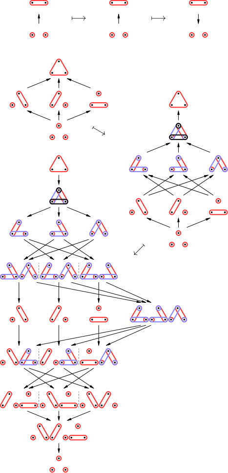 Figure 1
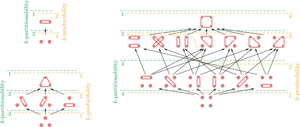 Figure 2
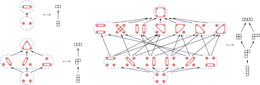 Figure 3
 Figure 4
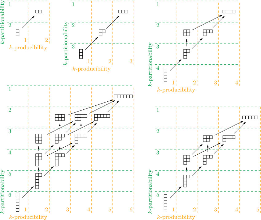 Figure 5
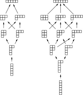 Figure 6
Peer Reviews
No public reviews on file for this paper yet. If you reviewed it on a platform where reviews are public (OpenReview, ICLR, NeurIPS, ICML), you can paste yours below so the community can read it here.
Videos
No videos yet. Explain this paper in a talk, walkthrough, or lecture? Add one.
k-stretchability of entanglement,
and the duality of k-separability and k-producibility
Szilárd Szalay
Strongly Correlated Systems “Lendület” Research Group, Wigner Research Centre for Physics, 29-33, Konkoly-Thege Miklós str., H-1121 Budapest, Hungary
Abstract
The notions of -separability and -producibility are useful and expressive tools for the characterization of entanglement in multipartite quantum systems, when a more detailed analysis would be infeasible or simply needless. In this work we reveal a partial duality between them, which is valid also for their correlation counterparts. This duality can be seen from a much wider perspective, when we consider the entanglement and correlation properties which are invariant under the permutations of the subsystems. These properties are labeled by Young diagrams, which we endow with a refinement-like partial order, to build up their classification scheme. This general treatment reveals a new property, which we call -stretchability, being sensitive in a balanced way to both the maximal size of correlated (or entangled) subsystems and the minimal number of subsystems uncorrelated with (or separable from) one another.
Contents
-
3 Multipartite correlation and entanglement: permutation invariant properties
-
5.1 -partitionability and -producibility of correlation and entanglement
-
5.4 Relations among -partitionability, -producibility and -stretchability
-
A On the structure of the classification of permutation invariant correlations
1 Introduction
The investigation of the correlations among the parts of a composite physical system is an essential tool in statistical physics. If the system is described by quantum mechanics, then nonclassical forms of correlations arise, the most notable is entanglement [1, 2, 3, 4]. It is the main resource of quantum information theory [5, 6, 7], and its nonclassical properties, playing important role also in many-body physics [8, 9, 10], make it influential in the behavior and characterization of strongly correlated systems [11, 12, 13, 14].
The correlation and entanglement between two parts of a system is relatively well-understood [15, 16, 17]. At least for pure states, the convertibility and the classification with respect to (S)LOCC ((stochastic) local operations and classical communication [17, 15, 18, 19]) shows a simple structure [20, 21], and there are basically unique correlation and entanglement measures [22, 23, 24]. The multipartite case is much more complicated [19, 25, 26, 27, 28]. Even for pure states, the nonexistence of a maximally entangled reference state [29, 30] and the involved nature of state-transformations in general [31, 32] seem to make the (S)LOCC-based classification practically unaccomplishable, and the standard (S)LOCC paradigm less enlightening so less expressive. Taking into account partial entanglement (partial separability) [33, 34, 35, 36, 37, 38, 39, 40], or partial correlations [14, 41, 42] only, leads to a combinatoric [43, 44, 45], discrete classification (based on the lattice of set partitions [44]), endowed naturally with a well-behaving set of correlation and entanglement measures, characterizing the finite number of properties [40, 14].
Even the partial correlation and partial entanglement properties are getting too involved rapidly, with the increasing of the number of subsystems. Singling out particularly expressive properties, we consider the -partitionability and -producibility of correlation and of entanglement. For subsystems, ranges from to , so the number of these properties scales linearly with the number of subsystems, moreover, their structures are the simplest possible ones, chains. (In the case of entanglement, -partitionability is called -separability [35, 37], while -producibility [46, 47, 48, 49] is also called entanglement depth [50, 51, 52]. Here we use both concepts for correlation and also for entanglement, this is why we use the naming “-partitionability of correlation” and “-producibility of correlation”, “-partitionability of entanglement” and “-producibility of entanglement” [40, 14, 41].) These characterize the strength of two different (one-parameter-) aspects of multipartite correlation and entanglement: those which cannot be restricted inside at least parts, and those which cannot be restricted inside parts of size at most , respectively. The concepts of -partitionability and -producibility of entanglement found application in spin chains [47, 48], appeared in quantum nonlocality [53], leading to device independent certification of them [54, 55], and were also demonstrated in quantum optical experiment [56]. -producibility also plays particularly important role in quantum metrology [57]. -producibly entangled states for larger lead to higher sensitivity, so better precision in phase estimation, which has been illustrated in experiments [58, 59, 60], and which also leads to -producibility entanglement criteria [61].
-partitionability and -producibility are special cases of properties invariant under the permutation of the subsystems. The permutation invariant correlation properties are based on the integer partitions [62, 45], also known (represented) as Young diagrams. For the description of the structure of these, we introduce a new order over the integer partitions, called refinement, induced by the refinement order over set partitions, used for the description of the structure of the partial correlation or entanglement properties [40]. The structure of the permutation invariant properties contains the chains of -partitionability and -producibility, and it is simpler than the structure describing all the properties. The number of these scales still rapidly with the number of subsystems, but slower than the number of all the partial correlation or entanglement properties.
The general treatment of the permutation invariant properties reveals a partial duality between -partitionability and -producibility, which is the manifestation of a duality on a deeper level, relating important properties of Young diagrams, by which -partitionability and -producibility are formulated.
The general treatment of the permutation invariant properties reveals also a particularly expressive new property, which we call -stretchability, leading to the definitions of “-stretchability of correlation” and “-stretchability of entanglement”. It combines the advantages of -partitionability and -producibility. Namely, -partitionability is about the number of subsystems uncorrelated with (or separable from) one another, and not sensitive to the size of correlated (or entangled) subsystems [47]; and -producibility is about the size of the largest correlated (or entangled) subsystem, and not sensitive to the number of subsystems uncorrelated with (or separable from) one another; while -stretchability is sensitive to both of these, in a balanced way. The price to pay for this is that we have roughly twice as many -stretchability properties, goes from to . However, -stretchability is linearly ordered with , while the relations between -partitionability and -producibility are far more complicated.
The organization of this work is as follows. In Section 2, we recall the structure of multipartite correlation and entanglement. In Section 3, we construct the parallel structure for the permutation invariant case. In Section 4, we show another introduction of the permutation invariant classification, which can although be considered simpler, but less transparent. In Section 5, we recall -partitionability and -producibility, introduce -stretchability, and show how these properties are related to each other. In Section 6, summary, remarks and open questions are listed. In Appendix A, we work out the “coarsening” step and some other tools, used in the main text. In Appendix B, we present the proofs of some further propositions given in the main text.
In the course of the presentation, the abstract mathematical structure of the correlation and entanglement properties (given in terms of lattice theoretic constructions) is well-separated from the concrete hierarchies of the state sets and measures. This leads to a transparent construction, which is easy to restrict to the permutation invariant case later. For the convenience of the reader, we provide a short summary on the notations. The abstract correlation and entanglement properties are labeled by Greek letters . On the three levels of the construction, these are typesetted as for the general case, and as for the permutation invariant case. On the first two levels of the construction, there are sets of quantum states of given correlation and entanglement properties, typesetted as , , , for the general case, and , , , for the permutation invariant case. On the first two levels of the construction, there are LO(CC)-monotonic measures of given correlation and entanglement properties, typesetted as , , , for the general case, and , , , for the permutation invariant case. On the third level of the construction, there are classes (disjoint sets) of quantum states of given correlation and entanglement properties, typesetted as , for the general case, and , for the permutation invariant case. The abstract correlation and entanglement properties are ordered, which is denoted by on the three levels of the construction in both the general and the permutation invariant cases. On the first two levels of the construction, thanks to the monotonicity properties, these manifest themselves as and for the state sets and for the measures, respectively. On the third level of the construction, these manifest themselves as LO(CC) conversion results, for which we do not introduce notation.
2 Multipartite correlation and entanglement
Here we recall the structure of the classification and quantification of multipartite correlation and entanglement [40, 14, 41]. Our goal is to do this in the way sufficient to see how the permutation invariant properties can be formulated parallel to this in the next section.
2.1 Level 0: subsystems
The classification scheme we present here is rather general. The elementary and composite subsystems can be any discrete finite systems possessing probabilistic description, supposed that the joint systems can be represented by the use of tensor products, which is the basic tool in the constructions. Such systems can be distinguishable quantum systems, second quantized bosonic systems, second quantized fermionic systems with fermion number parity superselection rule imposed, or even classical systems, with significant simplification in the structure in the latter case [41].
Let be the set of the labels of elementary subsystems. All the (possibly composite) subsystems are then labeled by the subsets , the set of which, , naturally possesses a Boolean lattice structure with respect to the inclusion , which is now denoted with . For every elementary subsystem , let the Hilbert space be associated with it, where . From these, for every subsystem , the Hilbert space associated with it is . (For the trivial subsystem , we have the one-dimensional Hilbert space [40].) The states of the subsystems are given by density operators (positive semidefinite operators of trace ) acting on , the sets of those are denoted with .
The mixedness of a state of a subsystem can be characterized by the von Neumann entropy [63, 64, 65, 7]
[TABLE]
The von Neumann entropy is monotone increasing in bistochastic quantum channels, and the relative entropy is monotone decreasing in quantum channels [67, 65, 6] and , .
2.2 Level I: set partitions
For handling the different possible splits of a composite system into subsystems, we need to use the mathematical notion of (set) partition [44] of the system . The partitions of are sets of subsystems,
[TABLE]
(For illustrations, see Figure 1.) This grabs our natural intuition of comparing splits of systems. Note that the refinement is a partial order only, there are pairs of partitions which cannot be ordered, for example, and , see Figure 1. (We use a simplified notation for the partitions, for example, , where this does not cause confusion.) Note that with the refinement is a lattice, with minimal and maximal elements and , and the least upper and greatest lower bounds, and , can be constructed [44, 45].
With respect to the partitions , we can define the partial correlation and entanglement properties, as well as the measures quantifying them.
The -uncorrelated states are those which are products with respect to the partition ,
[TABLE]
the others are -entangled states. (Here, and in the entire text, is a probability distribution, and .) The -separable states are exactly those which can be prepared from uncorrelated states by -local operations and classical communication among the parts . (This is abbreviated as -LOCC. With respect to the finest partition , we write simply LOCC.) Another point of view is that -separable states are exactly those which can be prepared from uncorrelated states by mixtures of -LOs. We also have that is closed under -LO, is closed under -LOCC [40, 41]. Clearly, if a state is product with respect to a partition, then it is also product with respect to any coarser partition, it is always free to forget about some tensor product signs. This means that these properties show the same lattice structure as the partitions [40, 41], , that is,
[TABLE]
One can define the corresponding (information-geometry based) correlation and entanglement measures [40, 14] for all -correlation and -entanglement. These are the most natural generalizations of the mutual information [6, 7], the entanglement entropy [16], and the entanglement of formation [17] for Level I of the multipartite case.
The -correlation of a state is its distinguishability by the relative entropy (1b) from the -uncorrelated states [70, 4, 40, 14],
[TABLE]
where is a pure decomposition of the state [40]. We have that is a correlation monotone (not increasing with respect to -LO, for the proof see Appendix B.1), is a strong entanglement monotone (convex and not increasing on average with respect to selective -LOCC [22, 23, 40]), and both of these are faithful, , [40], moreover, they show the same lattice structure as the partitions, , that is,
[TABLE]
which is called multipartite monotonicity [40, 14].
Note that, for two subsystems, for the only nontrivial partition , we have that is just two times the usual entanglement entropy. However, we have a way of derivation completely different than the usual, based on asymptotic LOCC convertibility from Bell-pairs [16]. The usual way cannot be generalized to the multipartite scenario (there is no “reference state”, which was the Bell-pair in the bipartite scenario), while our correlational, or statistical physical approach above could straightforwardly be generalized to the multipartite scenario not only here, but also for the Level II properties in the next subsystem.
2.3 Level II: multiple set partitions
In multipartite entanglement theory, it is necessary to handle mixtures of states uncorrelated with respect to different partitions [35, 37, 40]. For example, there are tripartite states which cannot be written as a mixture of a given kind of, e.g., -uncorrelated states, that is, not -separable, while can be written as a mixture of -uncorrelated and -uncorrelated states. Such states should not be considered fully tripartite-entangled, since there is no need for genuine tripartite entangled states in the mixture [35, 37, 39, 40]. Also, if a state is -separable and also -separable, it is not necessarily -separable. On the other hand, the order isomorphisms (4a)-(4b) tell us that if we consider states uncorrelated (or separable) with respect to a partition, then we automatically consider states uncorrelated (or separable) with respect to all finer partitions.
To embed these requirements in the labeling of the multipartite correlation and entanglement properties, we use the nonempty down-sets (nonempty ideals) of partitions [40], which are sets of partitions
[TABLE]
(For illustrations, see Figure 1.) The least upper and greatest lower bounds, and , are then the union and the intersection, and .
With respect to the partition ideals , we can define the partial correlation and entanglement properties, as well as the measures quantifying these.
The -uncorrelated states are those which are -uncorrelated (3a) with respect to a ,
[TABLE]
the others are -entangled states. The -separable states are exactly those which can be prepared from uncorrelated states by mixtures of -LOs for different partitions . (Note that such transformations do not form a semigroup.) We also have that is closed under LO, is closed under LOCC [40, 41]. It follows from (4) that these properties show the same lattice structure as the partition ideals [40], , that is,
[TABLE]
One can define the corresponding (information-geometry based) correlation and entanglement measures [40, 14] for all -correlation and -entanglement. These are the most natural generalizations of the mutual information [6, 7], the entanglement entropy [16], and the entanglement of formation [17] for Level II of the multipartite case.
The -correlation of a state is its distinguishability by the relative entropy (1b) from the -uncorrelated states [40, 14],
[TABLE]
We have that is a correlation monotone (for the proof, see Appendix B.1), is a strong entanglement monotone [40], and both of these are faithful, , [40], moreover, they show the same lattice structure as the partition ideals, , that is,
[TABLE]
which is called multipartite monotonicity for Level II [40, 14].
2.4 Level III: classes
The partial correlation and entanglement properties form an inclusion hierarchy (9a)-(9b), for example, if a state is -separable, then it is also -separable. We are interested in the labeling of the strict, or exclusive properties, for example, those states which are -separable and not -separable. In general, we would like to determine all the possible nonempty intersections of the state sets and . We call these intersections partial correlation and partial entanglement classes, containing states of well-defined partial correlation and partial entanglement properties.
To embed these requirements in the labeling of the strict properties of multipartite correlation and entanglement, we use the nonempty up-sets (nonempty filters) of nonempty down-sets (nonempty ideals) of partitions [40], which are sets of down-sets of partitions
[TABLE]
(For illustrations, see Figure 1.) Note that here, contrary to Level I and II, we call finer and coarser. In the generic case, if the inclusion of sets is described by a poset , then the possible intersections can be described by (for the proof, see appendix A.2 in [41]). One may make the classification coarser by selecting a subposet , with respect to which the classification is done, [40, 41].
With respect to the partition ideal filters , we can define the strict partial correlation and entanglement properties.
The strictly -uncorrelated states are those which are uncorrelated with respect to all , and correlated with respect to all , so the class of these (partial correlation class) is
[TABLE]
The meaning of the Level III hierarchy could also be clarified. If there exists a and an LO mapping it into , then [41, 40]; and if there exists a and an LOCC mapping it into , then [40]. In this sense, the Level III hierarchy compares the strength of correlation and entanglement among the classes.
The filters are sufficient for the description of the nontrivial classes (nonempty intersections) of the correlation and entanglement properties, but they are not necessary in general. For the strictly -uncorrelated states, the structure simplifies significantly [41]. (For example, for the finest classification , we have that the structure of the partial correlation classes is , as the unique labeling of the nontrivial partial correlation classes is given as for the partitions [41].) On the other hand, it is still a conjecture that -separability is nontrivial for all [40]. The conjecture holds for three subsystems, for which explicit examples were constructed [39, 73].
3 Multipartite correlation and entanglement: permutation invariant properties
Here we build up the structure of the classification and quantification of the permutation invariant multipartite correlation and entanglement properties. We do this from the point of view of the general properties in the previous section. To give a quick guidance on the construction, we show the diagram
[TABLE]
in advance. This might not seem to be obvious, for the proof, see Corollary 17 in Appendix A.4.
In Section 2, for the description of the structure of multipartite correlations [40, 14, 41], the natural language was that of set partitions [44]. For the permutation-invariant case, particularly -partitionability and -producibility, it is natural to use the simpler language of integer partitions [62, 45].
3.1 Level 0: subsystem sizes
Let us have the map, simply measuring the sizes of the subsystems ,
[TABLE]
mapping , which is simply
[TABLE]
This possesses the natural order , which is now denoted with , with respect to which is monotone, . We note for the sake of the analogy with the construction in the subsequent levels that one could define on as if there exist and such that , from which the monotonicity of follows automatically (see (64) in Appendix A.1).
3.2 Level I: integer partitions
Let the map in (15) act elementwisely on the partitions ,
[TABLE]
where on the right-hand side a multiset stays, that is, a set, which allows multiple instances of its elements. (For example, for , .) We call the integer partition the type of the set partition . This is then an integer partition of [62, 45], which is denoted as
[TABLE]
(For illustrations, see Figures 2 and 3. The integer partitions are represented by their Young diagrams, where the rows of boxes are ordered decreasingly.) This is a proper partial order (for the proof, see Appendix A.4). Note that the refinement is a partial order only, there are pairs of partitions which cannot be ordered, for example, and , see Figure 2. Note that with this partial order is not a lattice, since there are no unique least upper and greatest lower bounds with respect to that. (The first example is for , where , and there is no integer partition between them, see Figure 3.) The refinement also admits a minimal and a maximal element and . By construction, is monotone with respect to these partial orders, (see (64) in Appendix A.1).
With respect to the integer partitions , we can define the partial correlation and entanglement properties, as well as the measures quantifying them.
The -uncorrelated states are those which are -uncorrelated (3a) with respect to a partition of type , which is actually a Level II state set (8a) labeled by the ideal ,
[TABLE]
the others are -entangled states. The -separable states are exactly those which can be prepared from uncorrelated states by mixtures of -LOs for different partitions of type . We also have that is closed under LO, is closed under LOCC, because these hold for the general Level II state sets and , see in Section 2.3. It also follows that these properties show the same partially ordered structure as the integer partitions, , that is,
[TABLE]
(These come by using (74a) and (73a) in Appendix A.4, then (9) and (19).)
In accordance with the general case in Section 2.2, one can define the corresponding (information-geometry based) correlation and entanglement measures for all -correlation and -entanglement. These are the most natural generalizations of the mutual information [6, 7], the entanglement entropy [16], and the entanglement of formation [17] for Level I of the permutation invariant multipartite case.
The -correlation of a state is its distinguishability by the relative entropy (1b) from the -uncorrelated states, which is actually a Level II measure (10a) labeled by the ideal ,
[TABLE]
These inherit the properties of the general case in Section 2.3. So we have that is a correlation monotone, is a strong entanglement monotone, and both of these are faithful, , , moreover, they show the same partially ordered structure as the integer partitions, , that is,
[TABLE]
which we call multipartite monotonicity for Level I of the permutation invariant case. (These come by using (74a) and (73a) in Appendix A.4, then (11) and (21).)
3.3 Level II: multiple integer partitions
Let the map in (17) act elementwisely on the partition ideals ,
[TABLE]
where on the right-hand side a set stays. We call the type of the set partition ideal . This is a set of integer partitions, which is denoted as
[TABLE]
which turns out to be the inclusion, being the natural partial order for ideals. This might not seem to be obvious, this is given in (14), proven in Corollary 17 in Appendix A.4. (For illustrations, see Figure 4.) Because of these, with this partial order is a lattice. By construction, is monotone with respect to these partial orders, (see (64) in Appendix A.1).
With respect to the integer partition ideals , we can define the partial correlation and entanglement properties, as well as the measures quantifying these.
The -uncorrelated states are those which are -uncorrelated (3a) with respect to a partition of type for a , which is actually a Level II state set (8a) labeled by the ideal ,
[TABLE]
the others are -entangled states. The -separable states are exactly those which can be prepared from uncorrelated states by mixtures of -LOs for different partitions of different types . We also have that is closed under LO, is closed under LOCC, because these hold for the general Level II state sets and , see in Section 2.3. It also follows that these properties show the same lattice structure as the integer partition ideals, , that is,
[TABLE]
(These come by using (74b) and (73b) in Appendix A.4, then (9) and (25).)
In accordance with the general case in Section 2.3, one can define the corresponding (information-geometry based) correlation and entanglement measures for all -correlation and -entanglement. These are the most natural generalizations of the mutual information [6, 7], the entanglement entropy [16], and the entanglement of formation [17] for Level II of the permutation invariant multipartite case.
The -correlation of a state is its distinguishability by the relative entropy (1b) from the -uncorrelated states, which is actually a Level II measure (10a) labeled by the ideal ,
[TABLE]
These inherit the properties of of the general case in Section 2.3. So we have that is a correlation monotone, is a strong entanglement monotone, and both of these are faithful, , , moreover, they show the same lattice structure as the integer partition ideals, , that is,
[TABLE]
which we call multipartite monotonicity for Level II of the permutation invariant case. (These come by using (74b) and (73b) in Appendix A.4, then (11) and (27).)
3.4 Level III: classes
Let the map in (23) act elementwisely on the partition ideal filters ,
[TABLE]
where on the right-hand side a set stays. We call the type of the set partition ideal filter . This is a set of integer partition filters, which is denoted as
[TABLE]
which turns out to be the inclusion, being the natural partial order for filters. This might not seem to be obvious, this is given in (14), proven in Corollary 17 in Appendix A.4. (For illustrations, see Figure 4.) Note that here, contrary to Level I and II, we call finer and coarser. Because of these, with this partial order is a lattice. By construction, is monotone with respect to these partial orders, (see (64) in Appendix A.1).
With respect to the integer partition ideal filters , we can define the strict partial correlation and entanglement properties.
The strictly -uncorrelated states are those which are uncorrelated with respect to all , and correlated with respect to all , so the class of these (permutation invariant partial correlation class) is
[TABLE]
The meaning of the permutation invariant Level III hierarchy can also be clarified. If there exists a and an LO mapping it into , then ; and if there exists a and an LOCC mapping it into , then . In this sense, the permutation invariant Level III hierarchy compares the strength of correlation and entanglement among the permutation invariant classes. (These come by the analogue result for the general case in Section 2.4, for the coarsened classification based on the permutation invariant properties , see in the next section.)
4 An alternative way of introducing permutation invariance
The Level II structure encodes the different partial correlation and entanglement properties. In Sections 2 and 3, we have built up the structure of the classification, parallel for the general, and for the permutation invariant cases. Here we show a more compact, but less transparent treatment of the same structure, by embedding both constructions into .
The three-level building of the correlation and entanglement classification was given by the construction
[TABLE]
in Section 2. Because of (4), one may embed into , using the principal ideals in ,
[TABLE]
In this way, is a sublattice of .
The same can be done for the permutation invariant correlation and entanglement classification given by the construction
[TABLE]
in Section 3. In the same way, because of (20), one may embed into , using the principal ideals in ,
[TABLE]
In this way, is a sublattice of .
The third point here is that, noting that (for the proof, see (73a) in Appendix A.4), one may also embed (thus also ) into , using
[TABLE]
(For the proof, see (74a) and (74b) in Appendix A.4.) In this way, and are sublattices of .
A is permutation invariant, if and only if . (Then describes the same property as .) So can be given directly as
[TABLE]
and the permutation invariant classification can be described as a coarsened classification with respect to the permutation invariant properties .
We note that could also be embedded into by principal filters (and similarly into ), however, the construction has led to a different direction.
5 -partitionability, -producibility and -stretchability
In this section, we consider -partitionability and -producibility as particular cases of permutation invariant properties of partial correlation and entanglement, and elaborate a duality between them. Our point of view makes possible to reveal a new property, which we call -stretchability, combining some advantages of -partitionability and -producibility. We also investigate the relations among these three properties.
5.1 -partitionability and -producibility of correlation and entanglement
-partitionability and -producibility are permutation invariant Level II properties. A partition is -partitionable, if the number of its parts is at least , while it is -producible, if the sizes of its parts are at most . (For illustration, see Figure 5.) These are encoded by the ideals of -partitionable and -producible partitions,
[TABLE]
for , forming chains in the lattice ,
[TABLE]
Since -partitionability and -producibility are permutation invariant properties, it is enough to consider their types (23)
[TABLE]
forming chains in the lattice ,
[TABLE]
The corresponding -partitionably uncorrelated and -producibly uncorrelated states (25a) are
[TABLE]
which can be decomposed into -partitionably, or -producibly uncorrelated states, respectively. Because of (26a), these properties show the same chain structure as the chains of the corresponding partition ideals (39), that is,
[TABLE]
that is, if a state is -partitionably uncorrelated (separable) then it is also -partitionably uncorrelated (separable) for all , and if a state is -producibly uncorrelated (separable) then it is also -producibly uncorrelated (separable) for all .
The corresponding -partitionability correlation and -producibility correlation (27a) are [14]
[TABLE]
Because of (28), these measures show the same chain structure as the chains of the corresponding partition ideals (39), that is,
[TABLE]
that is, -partitionability correlation (entanglement) is always stronger than -partitionability correlation (entanglement) for all , and -producibility correlation (entanglement) is always stronger than -producibility correlation (entanglement) for all , which is the multipartite monotonicity of these measures.
For the labeling of the strict partitionability and producibility properties, we have the ideal filters
[TABLE]
by (36) and (37). The corresponding strictly -partitionably uncorrelated and strictly -producibly uncorrelated states (31a) are
[TABLE]
which can be decomposed into -partitionably but not -partitionably, and -producibly but not -producibly uncorrelated states, respectively. ( and are understood.)
5.2 Duality by conjugation
Looking at the -partitionability and -producibility properties in Figure 5, and also at their definitions (36a) and (36b), it is not clear how these are related to each other.
In Section 3, the permutation invariant correlation properties were described by the use of integer partitions, represented by Young diagrams in the figures. Important properties of Young diagrams are their height, width and rank, given for an integer partition as
[TABLE]
and also for set partition as , , . It is enlightening now to arrange the poset according to the height and width of the partitions, in the way as can be seen in Figure 6, i.e., the height is increasing downwards, the width is increasing to the right, then the rank is increasing up-right. It is easy to see that the height is strictly decreasing, the width is increasing, and the rank is strictly increasing monotone with respect to the refinement (18c),
[TABLE]
(For illustration, see Figure 6: the arrows point always upwards, and possibly to the up-right, never to the up-left, horizontally or downwards.)
Now the partitionability and producibility properties (36a) and (36b) can be formulated with the height and width as
[TABLE]
On the set of Young diagrams, an involution arises naturally, called conjugation, being the reflection of the diagram with respect to its “diagonal” [45]. Considering the integer partitions themselves, the conjugation is given as follows. For decreasingly ordered values of the elements of , the number of elements that equal to is in the conjugated partition (setting for ). With multisets, the conjugation is given as the map ,
[TABLE]
where both sets on the right-hand side are multisets.
The partial order (18c) does not show nice properties with respect to the conjugation. (For illustration, see the height-width based arrangement in Figure 6.) The conjugation is not an anti-automorphism, if then it does not follow that (the first example is for , where we have and ). The conjugation is neither an automorphism of course, if then it does not follow that (the first example is for , where we have and ). An integer partition and its conjugate cannot be ordered by refinement (the first example is for , where we have and , which are conjugates of each other, and cannot be ordered).
The conjugation interchanges the height and width, and multiplies the rank with ,
[TABLE]
(For illustration, see the height-width based arrangement in Figure 6: the conjugation brings to the position mirrored with respect to the diagonal .) Note that, although the conjugation interchanges the height and width, it does not interchange the partitionability (48a) and producibility (48b) properties, since these are given in different ways by height and width, namely, by lower and upper bounds.
5.3 -stretchability of correlation and entanglement
In Section 5.2, we introduced the permutation invariant property -stretchability (48c) for . Because of the third inequality in (47), these form a chain in the lattice ,
[TABLE]
(For illustration, see the height-width based arrangement in Figure 6.)
The corresponding -stretchably uncorrelated states (25a) are
[TABLE]
which can be decomposed into -stretchably uncorrelated states. Because of (26a), these properties show the same chain structure as the chains of the corresponding partition ideals (51), that is,
[TABLE]
that is, if a state is -stretchably uncorrelated (separable) then it is also -stretchably uncorrelated (separable) for all .
The corresponding -stretchability correlation (27a) is
[TABLE]
Because of (28), these measures show the same chain structure as the chain of the corresponding partition ideals (51), that is,
[TABLE]
that is, -stretchability correlation (entanglement) is always stronger than -stretchability correlation (entanglement) for all , which is the multipartite monotonicity of these measures.
For the labeling of the strict stretchability properties, we have the ideal filters
[TABLE]
by (48c) and (51). The corresponding strictly -stretchably uncorrelated states (31a) are
[TABLE]
which can be decomposed into -stretchably but not -stretchably uncorrelated states. ( is understood.)
-partitionability (48a), -producibility (48b) and -stretchability (48c) give, of course, a rather coarsened description of permutation invariant correlation or entanglement properties. Because of this, they must show some disadvantages. First, -partitionability (48a) takes into account only the number of subsystems uncorrelated with (or separable from) one another, and does not distinguish between the cases when subsystems of roughly equal sizes are uncorrelated (or separable), and when some elementary subsystems are uncorrelated with (or separable from) the rest of a large system, although these two cases represent highly different situations form a resource-theoretical point of view. (For illustration, see the rows in Figure 6.) Second, -producibility (48b) takes into account only the size of the largest subsystem uncorrelated with (or separable from) the other part of the system, and does not distinguish between the cases when a large subsystem is uncorrelated with (or separable from) a slightly smaller subsystem, or many elementary subsystems, although these two cases represent again highly different situations form a resource-theoretical point of view. (For illustration, see the columns in Figure 6.) Third, -stretchability (48c) combines the advantages of the previous two properties in a balanced way, it takes into account a kind of “difference” of them, and does not distinguish among cases with rather different types. (For illustration, see the lines parallel to the diagonal in Figure 6.)
5.4 Relations among -partitionability, -producibility and -stretchability
The height , width and rank (46) of the integer partitions of are bounded by one another as
[TABLE]
The first inequality in (58a) can be seen by noting that , because the right-hand side is the area of the smallest rectangle into which the Young diagram of boxes fits. The second inequality in (58a) can be seen by noting that , because the left-hand side is the half circumference of the smallest rectangle into which the Young diagram of boxes fits. The inequalities in (58b) come by the same reasoning, or by conjugation (50) in (58a). The inequalities in (58c) come by subtracting from (58b). The inequalities in (58d) come by an analogous reasoning, or by conjugation (50) in (58c). The inequalities in (58e) come by solving the respective inequalities in (58c) for . The inequalities in (58f) come by an analogous reasoning, or by conjugation (50) in (58e).
The first inequality in (58d) and the second inequalities in the others in (58) are saturated for the partition , where the integer occurs times. The second inequality in (58d) and the first inequalities in the others in (58) are saturated for the partition , where the integer occurs times. In the cases where noninteger value stays on one side of an inequality, saturation is understood for the inequality strengthened by the ceiling or floor functions or ; that is, if , then also , and if , then also . (For illustration, see Figure 6. The second inequalities in (58a) and (58b) express that the arrangement of Young diagrams in Figure 6 is “skew upper triangular”, while the first inequalities in (58a) and (58b) describe the “hyperbolic” shape of the upper boundary. The other inequalities in (58) give the boundaries in the rank-height or width-rank plane.)
Since the partitionability is related to lower-bounding the height (48a), the producibility is related to upper-bounding the width (48b), and the stretchability is related to their difference (48c), the bounds in (58) lead to the following relations between these properties
[TABLE]
The relations in (59a) and (59b) can be seen by using the second inequality in (58b) and the second inequality in (58c), respectively, with (48a). The relations in (59c) and (59d) can be seen by using the first inequality in (58a) and the second inequality in (58d), respectively, with (48b). (For noninteger values, strengthening by the ceiling function was also exploited, as before.) The relations in (59e) and (59f) can be seen by using the first inequality in (58e) and the second inequality in (58f), respectively, with (48c).
From the relations (59), for the inclusion of the state spaces (40), we have
[TABLE]
by the order isomorphisms (26); and for the bounds of the measures (42), we have
[TABLE]
by the multipartite monotonicity (28).
6 Summary, remarks and open questions
In this work we investigated the partial correlation and entanglement properties which are invariant under the permutations of the subsystems. The set partition based three-level structure, describing the classification of partial correlation and entanglement (Section 2) was mapped to a parallel, integer partition based three-level structure, describing the permutation invariant case (Section 3). This mapping is easy to understand on Level I of the construction, however, to see that it is working well through the whole construction, a formal proof was given (Appendix A). The construction can be made more compact, although less transparent (Section 4), which can be used as a starting point of more advanced investigations.
We also investigated -partitionability and -producibility, fitting naturally into the structure of permutation invariant properties. A kind of combination of these two gives -stretchability, which is sensitive in a balanced way to both the maximal size of correlated (or entangled) subsystems and the minimal number of subsystems uncorrelated with (or separable from) one another. We studied their relations, and a duality, connecting the former two (Section 5).
In the following, we list some remarks and open questions.
The first point to note is that we have followed a treatment of entanglement, which is somewhat different than the standard LOCC paradigm [15]. The LOCC paradigm grabs the essence of entanglement as a correlation which cannot be created or increased by classical communication (classical interaction). This point of view leads to a classification too detailed and practically unaccomplishable for the multipartite scenario. Our treatment is rooted more in statistics, by noticing that (i) pure states of classical systems are always uncorrelated, so in pure states, correlations are of quantum origin, and this is what we call entanglement [1]; and (ii) mixed states of classical systems can always be formed by forgetting about the identity of pure (hence uncorrelated) states, so in mixed states, correlations which cannot be described in this way are of quantum origin, and this is what we call entanglement. These principles are working painlessly in the multipartite scenario, entangled states and correlation based definitions of entanglement measures were defined based on these in the first two levels of the structure of multipartite entanglement. In particular, from (i) it follows that entanglement in pure states should be measured by correlation (see (5b) and (10b), and the corresponding quantities for the permutation invariant case, and the notes in the end of Section 2.2). We emphasize that this statistical point of view is fully compatible with LOCC, and has led to a much coarser, finite classification.
Being uncertain (or forgetting) about the identity of the state of the system is a guiding principle in the definition of the different aspects of multipartite entanglement in Section 2 (see also in point (ii) in Section VII.A. in [40]).
States in : We are uncertain about the (pure) state, by which the system is described (Section 2.1).
States in (): We are uncertain about the pure state, by which the system is described, but we are certain about the partition with respect to which the state is uncorrelated (separable) (Section 2.2).
States in (): We are uncertain about the pure state, by which the system is described, and we are also uncertain about the partition with respect to which the state is uncorrelated (separable), but we are certain about the possible partitions with respect to which the state is uncorrelated (separable) (Section 2.3).
States in (): We are uncertain about the pure state, by which the system is described, and we are also uncertain about the partition with respect to which the state is uncorrelated (separable), but we are certain about the possible partitions with respect to which the state is uncorrelated (separable), and we are also certain about the possible partitions with respect to which the state is correlated (entangled) (Section 2.4).
We also mention here that for the state sets of given multipartite correlation (entanglement) properties (), except from the fully uncorrelated (or fully separable) case , we cannot formulate semigroups of quantum channels which could play the role of “free operations” for these “free state” sets in a usual resource-theoretical scenario [75]. Instead of this, being uncertain (or forgetting) about the identity of the maps is the guiding principle here (see the characterizations in Sections 2.2 and 2.3, as well as in the permutation invariant case in Sections 3.2 and 3.3). Note that this is physical: only the fully uncorrelated (fully separable) states are for free, the others are resource states, possibly of different “value.”
Note that, after the general case (Section 2), we considered the permutation invariant (correlation or entanglement) properties (from Section 3). The use of these is not restricted to permutation invariant states: these are simply the permutation invariant properties of also non-permutation-invariant states. If the states considered are permutation invariant (for example, in the first quantization of bosonic or fermionic systems), then these are the only relevant properties.
The permutation invariant properties were described by the use of integer partitions, for which a refinement-like order was given, which is just the coarsening of the refinement order of set partitions. In the literature, there are several partial orders constructed for integer partitions, such as the dominance order [76] (based on majorization, leading to a lattice), the Young order [62, 45] (based on diagram containment, given for partitions of all integers, leading to Young’s lattice, here partitions of the same integer cannot be ordered, and the order is invariant to the conjugation), or the reverse lexicographic order (leading to a chain). The refinement order for integer partitions, introduced in (18c) through the refinement order for set partitions (2c), is different from the above orders, and, to our knowledge [62, 45], was not considered upon its merits in the literature before. Although Birkhoff mentioned this partial order in his book [77] as an example, it was not used for any reasonable purpose. The reason for this might be that the resulting poset shows properties not so nice or powerful as those shown by the others. However, this order is what needed is in the classification problem of permutation invariant properties, that is reflected also by the monotonicities (47).
-partitionability is about the natural gradation of the lattice of set partitions or of the poset of integer partitions , but it was not clear, how -producibility can be understood. The conjugation of integer partitions has explained the role of the latter, by establishing a kind of duality between the two properties. Note, however, that this duality is only partial: although the conjugation of integer partitions (49) interchanges the height and the width (50), by which the -partitionability and -producibility properties are given, but the latter properties are given in an opposite way by height and width, see (48a) and (48b). So the conjugation does not interchange -partitionability and -producibility, it establishes a connection on the deeper level of integer partitions only. This is also reflected in the relations among the different -partitionability and -producibility properties, given in (59a) and (59c).
For , the height and width determine uniquely. For , we have and , being of height and width . Note that two different integer partitions of the same height and width can never be ordered. (Ordered pairs are of different height, because of the strict monotonicity of the height (47).)
The property of -stretchability (48c) was introduced by the rank of the partition. We note that the rank of an integer partition (46c) was defined and used originally in a very different context in number theory and combinatorics. It was introduced by Freeman Dyson [78] in his investigations of Ramanujan’s congruences in the partition function [74].
For subsystems, the number of nontrivial -partitionability and -producibility properties is in both cases (-partitionability and -producibility are trivial), while the number of nontrivial -stretchability properties is (-stretchability is trivial). All of these three properties form chains, see (39a), (39b) and (51), and the relations among them are given in (59). Note that -stretchability combines the advantages of -partitionability and -producibility, in the sense that it rewards large correlated (or entangled) subsystems, while it punishes the larger number of subsystems uncorrelated (or separable) with one another. Also, while the relations between -partitionability and -producibility are highly nontrivial (59a), (59c), the -stretchability properties form a chain (51). The price to pay for this is that sometimes there are rather different properties not distinguished by stretchability, for example, and are both -stretchable. Taking stretchability seriously leads to a highly nontrivial, balanced comparison of permutation invariant multipartite correlation or entanglement properties.
Discussions with Géza Tóth and Mihály Máté are gratefully acknowledged. This research was financially supported by the National Research, Development and Innovation Fund of Hungary within the Researcher-initiated Research Program (project Nr: NKFIH-K120569) and within the Quantum Technology National Excellence Program (project Nr: 2017-1.2.1-NKP-2017-00001), the Ministry for Innovation and Technology within the ÚNKP-19-4 New National Excellence Program, and the Hungarian Academy of Sciences within the János Bolyai Research Scholarship and the “Lendület” Program.
Appendix A On the structure of the classification of permutation invariant correlations
A.1 Coarsening a poset
Let us have a finite set endowed with a binary relation , and a function , mapping to . (In the appendix we consider finite sets only, even if it is not mentioned explicitly.) The same function transforms also the relation naturally as follows. A binary relation can be considered as a set of ordered pairs in , written as , then by the elementwise action of . We use the shorthand notation for this. The meaning of this is that
[TABLE]
(Here denotes the inverse image of the singleton .)
If the binary relation is a partial order [43, 45], the transformed one is not necessarily that. To make it a partial order, we need some constraints imposed on . Let us introduce the following three conditions:
[TABLE]
These conditions, although being rather strong, hold in the construction in which we need them (see Appendix A.4, and Lemma 16). They turn out to be sufficient for to be a partial order, as the following lemma states.
Lemma 1**.**
Let be a poset, then is a poset if (63a) and (63c) hold, or if (63b) and (63c) hold.
Proof.
We need to prove that is a partial order in these cases.
(i) Reflexivity (, ): for all we have , since is surjective, and we need and for which by (LABEL:eq:relp); this holds for the choice , since the partial order is reflexive, . (This proof does not use any of the constraints (63).)
(ii) Antisymmetry (, if and , then ): let , which means that there exist and such that , by (LABEL:eq:relp). Fix such a pair and . Also, let , applying (63a) for , we have that there exists , such that . Then, applying (63c) to , we have that . (This proof uses (63a) and (63c). A similar proof can be given by using (63b) and (63c).)
(iii) Transitivity (, if and , then ): let , which means that there exist and such that , by (LABEL:eq:relp). Fix such a pair and . Also, let , applying (63a) for , we have that there exists , such that . Then, since the partial order is transitive, we have that for an and , which means that by (LABEL:eq:relp). (This proof uses (63a). A similar proof can be given by using (63b).) ∎
The following construction would be much simpler if the conditions (63) would also be necessary. Note that this is not the case: if is a partial order, then (63c) holds, but (63a) and (63b) do not hold. For example, for the poset with the only arrow , and the function given as , we have , but (63a) does not hold.
If (63a) or (63b), and (63c) hold, then the new poset can be considered as a coarsening of by . ( is surjective by definition. If it is also injective, then and are isomorphic, and the coarsening is trivial.) Note that, because of the construction, is automatically monotone,
[TABLE]
(Indeed, and , so (LABEL:eq:relp) holds.) Note also that, if the poset is a lattice, the transformed one is not necessarily that. To make it a lattice, further conditions have to be imposed; this problem is not addressed here.
A.2 Down-sets and up-sets
In a poset , a down-set (order ideal) is a subset , which is closed downwards [43, 45],
[TABLE]
These form lattices with respect to the inclusion , with the join (least upper bound), being the union , and the meet (greatest lower bound), being the intersection .
As in the previous section, let us have the poset , the function , by which , and for which (63a) or (63b), and (63c) hold. Additionally, let have bottom and top elements. (Then also has bottom and top elements. Indeed, this is because the bottom and top elements in are mapped to the bottom and top elements in , because of the (64) monotonicity of .) Now let us form from the posets and the lattices of nonempty down-sets
[TABLE]
(The existence of the bottom elements in and ensures that not only the down-sets but also the nonempty down-sets form lattices in both cases [40].) Then, by denoting the elementwise action of with , that is, , in the following lemmas we will show that , that is, the diagram
[TABLE]
commutes. Here is the partial order transformed by in the same way as was transformed by in (LABEL:eq:relp), and we also have automatically that is monotone for and , in the same way as in (64).
The following two technical lemmas concerning the sets will be used several times later.
Lemma 2**.**
In the above setting (and assuming (63)), for all , we have g\bigl{(}\bigcup_{a^{\prime}\in\mathbf{a}^{\prime}}f^{-1}(a^{\prime})\bigr{)}=\mathbf{a}^{\prime}.
Proof.
This is because is the elementwise action of , so g\bigl{(}\bigcup_{a^{\prime}\in\mathbf{a}^{\prime}}f^{-1}(a^{\prime})\bigr{)}=g\bigl{(}\bigcup_{a^{\prime}\in\mathbf{a}^{\prime}}\{a\in P\;|\;f(a)=a^{\prime}\}\bigr{)}=\bigcup_{a^{\prime}\in\mathbf{a}^{\prime}}g\bigl{(}\{a\in P\;|\;f(a)=a^{\prime}\}\bigr{)}=\bigcup_{a^{\prime}\in\mathbf{a}^{\prime}}\{a^{\prime}\}=\mathbf{a}^{\prime}. ∎
Lemma 3**.**
In the above setting (and assuming (63)), for all , we have , that is, it is a nonempty down-set.
Proof.
First, denote . On the one hand, , since and is surjective. On the other hand, if for an , then because of the monotonicity (64). Since by the construction of , and is a down-set (65a), we have that . Then by the construction of , and then , so is a down-set. Altogether we have that . ∎
The following two lemmas show (67).
Lemma 4**.**
In the above setting (and assuming (63)), we have .
Proof.
We need to prove both inclusions.
(i) We need that . Let and . Then for all let us have . (Note that by construction.) Then let , and applying (63a) for , we have that there exists such that . Since , and is a down-set (65a), we have that , and then , so is a down-set.
(ii) We also need that . Let , then we construct an , for which . The element fulfills these criteria, we have by Lemma 2, and by Lemma 3. ∎
Lemma 5**.**
In the above setting (and assuming (63)), we have .
Proof.
We need to prove both directions.
(i) We need that for all , if then . means that and such that . (Again, is the inverse image of the singleton .) In this case, , so .
(ii) We also need that for all , if then . From and , let us form and . We have that and (they are nonempty down-sets) by Lemma 3, also and by Lemma 2, and if then by construction. That is, we have constructed and , for which , so we have . ∎
Summing up, Lemma 4 and Lemma 5 together state that (67) commutes. Later we also need that the properties (63a), (63b) and (63c) are inherited.
Lemma 6**.**
In the above setting (and assuming (63)), we have
[TABLE]
Proof.
(68a) can be proven by the explicit construction of . Let , and , then \mathbf{b}:=\bigl{(}\bigcup_{b^{\prime}\in\mathbf{b}^{\prime}}f^{-1}(b^{\prime})\bigr{)}\cap\mathbf{a}. By construction, . Also, , that is, it is a nonempty down-set, since it is the intersection (meet) of two nonempty down-sets: , and by Lemma 3, and is a lattice. In addition, we need that , that is, . Since , we have that , such that . Then also , such that , that is, , and also , so by construction of .
(68b) can be proven analogously.
(68c) is a simple consequence of the properties of . Let , then by the monotonicity of , so by the transitivity and antisymmetry of the partial order , if then .
Note that the conditions (63) were not used explicitly in these proofs, they are assumed only for establishing the partial order for the set , see Lemma 1. ∎
Lemma 7**.**
Lemmas 2, 3, 4, 5 and 6, hold also if up-sets are used instead of down-sets in the construction (67).
Proof.
All the proofs can be repeated with slight modifications, as interchanging the roles of (63a) and (63b), down-closures and up-closures, and reversing orders. ∎
Thanks to Lemma 4, Lemma 5, Lemma 6 and Lemma 7, the construction (67) can be repeated arbitrary times, with either up- or down-sets, if the conditions (63) hold for the first level. Note that and are partial orders by construction anyway. The inheritance of (63), shown in Lemma 6 is needed not for that, but also for, e.g., Lemma 4, when applied for the next level.
A.3 Embedding
Now, with the definition (66), let the function be given as
[TABLE]
and its image . We will show that this is a subposet, and , and is an embedding of into . (We use the notation for any subset of a lattice.)
The following two technical lemmas concerning the images will be used several times later.
Lemma 8**.**
In the above setting (and assuming (63)), for all , we have
[TABLE]
Proof.
(70a) is by definition , and we need to prove both inclusions. First, holds, since is the elementwise action of . Second, for , we need to see that for all such that there exists an for which , while . The element fulfills these criteria, we have by Lemma 2, and by Lemma 3; while , since , so it appears in the union .
(70b) can be proven by noting that for the left-hand side, we have by (70a) that g^{\prime}(\mathbf{a}^{\prime})=\bigl{\{}a\in P\;\big{|}\;f(a)\in\mathbf{a}^{\prime}\bigr{\}}\equiv\{a\in P\;|\;\exists a^{\prime}\in\mathbf{a}^{\prime}\;\;\text{s.t.}\;\;f(a)=a^{\prime}\}, which is the same as the right-hand side . ∎
Lemma 9**.**
In the above setting (and assuming (63)), for all , we have .
Proof.
Using (70b), we have that g(g^{\prime}(\mathbf{a}^{\prime}))=g\bigl{(}\bigcup_{a^{\prime}\in\mathbf{a}^{\prime}}f^{-1}(a^{\prime})\bigr{)}, then Lemma 2 leads to the claim. ∎
The following lemma shows that is an embedding of into .
Lemma 10**.**
In the above setting (and assuming (63)), .
Proof.
We need to prove that for all , , then, from the antisymmetry of the partial order, we have that is bijective.
To see the “if” direction, we have then by the monotonicity of , similarly to (64), then by Lemma 9.
To see the “only if” direction, we have , then , then by (70a). ∎
In the following four lemmas, we provide some simple tools, concerning principal ideals.
Lemma 11**.**
In the above setting (and assuming (63)), for all , we have .
Proof.
For the left-hand side we have , while for the right-hand side we have , by definitions. So we need that for all and , .
To see the “if” direction, we have that if then for there exists such that by (63a).
To see the “only if” direction, we have that if such that , then by the monotonicity (64) of , then , since by the assumption . ∎
Lemma 12**.**
In the above setting (and assuming (63)), for all , we have .
Proof.
For the left-hand side we have by applying (70a), while for the right-hand side we have , by definitions. So we need that for all and .
To see the “if” direction, we have that if then for there exists such that by (63b).
To see the “only if” direction, we have that if such that , then by the monotonicity (64) of , then , since by the assumption . ∎
Lemma 13**.**
In the above setting (and assuming (63)), for all , we have .
Proof.
First, we have obviously. Second, we have , which is a special case of Lemma 10, for principal ideals in . ∎
Lemma 14**.**
In the above setting (and assuming (63)), for all , we have
[TABLE]
Proof.
We have , by using Lemma 12, (70b), exploiting that is a down-set (65a), then (70b) again, respectively. ∎
Although it will not be used, the following lemma shows that the whole construction in this section works also if up-sets are used instead of down-sets.
Lemma 15**.**
Lemmas 8, 9, 10, 11, 12, 13 and 14 hold also if up-sets are used instead of down-sets in the construction (67).
Proof.
All the proofs can be repeated with slight modifications. ∎
A.4 Application to the set and integer partitions
Now we turn to the case of the main text, for which the machinery developed in the previous sections is applied. That is, for the roles of and we have the poset of set partitions (2b) with the refinement relation (2c), and the poset of integer partitions (18b) with the refinement relation (18c).
First, we have the permutations of the elementary subsystems , acting naturally on the partitions as \sigma(\xi)=\bigl{\{}\{\sigma(i)\;|\;i\in X\}\;\big{|}\;X\in\xi\bigr{\}}\in P_{\text{I}}. We will make use of the obvious observations that all the permutations of a partition are of the same type, ; and all partitions of a given type can be transformed into one another by suitable permutations, that is, for all , there exists at least one by which . Also, for all permutations, if and only if . Using these, we can show that (63)-like conditions hold for this case.
Lemma 16**.**
In the setting of the main text, the following conditions hold
[TABLE]
Proof.
Recall that by definition if there exist and , such that , see (18c), in accordance with (LABEL:eq:relp). Then, for all we can construct which is , simply as by any of the permutations implementing , leading to (72a).
(72b) can be proven analogously.
(72c) can be proven by noting that for all we have that if then , by (2c); and , by (17). Then and lead to with , form which we have . Now we need that and lead to (then ), which holds, because (2c) must be fulfilled with the same number of parts: let us number them accordingly as for and , with the constraints of being disjoint and , which leads to . ∎
Recall that Lemma 1 states that if a poset is transformed by a function as given in (LABEL:eq:relp), then is a poset if the conditions (63) hold. Now Lemma 16 shows that for the poset , if transformed by as given in (18b) and (18c) in the main text, the corresponding conditions (72) hold, so is a poset.
Recall also that if we form the down-set lattices (66), then Lemma 4 and Lemma 5 together state that (67) commutes, Lemma 6 states that the conditions in (63) are inherited. Then with Lemma 7, we have that in the main text, the three-level construction is well-defined as follows.
Corollary 17**.**
The diagram (14) in the main text commutes.
With Lemma 12 and (71), we also have that for the first two levels of the construction in the main text, the following identities concerning the principal ideals hold.
Corollary 18**.**
In the setting of the main text, for all and , we have
[TABLE]
With Lemma 13 and Lemma 10, we also have that for the first two levels of the construction in the main text, the following order isomorphisms hold.
Corollary 19**.**
In the setting of the main text, for all and , we have
[TABLE]
Appendix B Miscellaneous proofs
B.1 Monotonicity of correlation measures
Here we show the -LO monotonicity of the -correlation (5a), from which the LO monotonicity of the -correlation (10a) follows, because the latter one is a minimum of some of the former ones. A quantum channel (completely positive trace preserving map [6, 7]) is -LO, if it can be written as with quantum channels for all . With this,
[TABLE]
where the first inequality comes from
[TABLE]
which holds for -LOs; and the second inequality comes from the monotonicity of the relative entropy (1b),
[TABLE]
which holds for all quantum channels [6, 7].
Note that the monotonicity shown here is a particular case of a much more general property of monotone distance based geometric measures [65] in resource theories [75]: the monotonicity with respect to free maps, by which the set of free states is mapped onto itself.
The reference list from the paper itself. Each links out to its DOI / PubMed record.
- 1Schrödinger [1935 a] Ervin Schrödinger. Die gegenwärtige Situation in der Quantenmechanik. Naturwissenschaften , 23:807, 1935 a. doi: 10.1007/BF 01491987 .
- 2Schrödinger [1935 b] Ervin Schrödinger. Discussion of probability relations between separated systems. Math. Proc. Camb. Phil. Soc. , 31:555, 1935 b. doi: 10.1017/S 0305004100013554 .
- 3Horodecki et al. [2009] Ryszard Horodecki, Paweł Horodecki, Michał Horodecki, and Karol Horodecki. Quantum entanglement. Rev. Mod. Phys. , 81(2):865–942, Jun 2009. doi: 10.1103/Rev Mod Phys.81.865 .
- 4Modi et al. [2010] Kavan Modi, Tomasz Paterek, Wonmin Son, Vlatko Vedral, and Mark Williamson. Unified view of quantum and classical correlations. Phys. Rev. Lett. , 104:080501, Feb 2010. doi: 10.1103/Phys Rev Lett.104.080501 .
- 5Nielsen and Chuang [2000] Michael A. Nielsen and Isaac L. Chuang. Quantum Computation and Quantum Information . Cambridge University Press, 1 edition, October 2000. ISBN 0521635039. doi: 10.1017/CBO 9780511976667 .
- 6Petz [2008] Dénes Petz. Quantum Information Theory and Quantum Statistics . Springer, 2008. doi: 10.1007/978-3-540-74636-2 .
- 7Wilde [2013] Mark M. Wilde. Quantum Information Theory . Cambridge University Press, 2013. doi: 10.1017/CBO 9781139525343 .
- 8Coffman et al. [2000] Valerie Coffman, Joydip Kundu, and William K. Wootters. Distributed entanglement. Phys. Rev. A , 61:052306, Apr 2000. doi: 10.1103/Phys Rev A.61.052306 .