TL;DR
This paper develops methods to quantify uncertainty in patient-specific survival curves generated by individual survival distribution models, enhancing their clinical utility with accurate prediction intervals.
Contribution
It adapts existing sampling-based methods and introduces new techniques for estimating simultaneous prediction intervals for survival curves, applicable beyond survival analysis.
Findings
Existing method adapted for survival curve intervals
New methods provide competitive interval estimation performance
Applicable to any context with tractable sampling of the distribution
Abstract
Accurate models of patient survival probabilities provide important information to clinicians prescribing care for life-threatening and terminal ailments. A recently developed class of models - known as individual survival distributions (ISDs) - produces patient-specific survival functions that offer greater descriptive power of patient outcomes than was previously possible. Unfortunately, at the time of writing, ISD models almost universally lack uncertainty quantification. In this paper, we demonstrate that an existing method for estimating simultaneous prediction intervals from samples can easily be adapted for patient-specific survival curve analysis and yields accurate results. Furthermore, we introduce both a modification to the existing method and a novel method for estimating simultaneous prediction intervals and show that they offer competitive performance. It is worth…
Click any figure to enlarge with its caption.
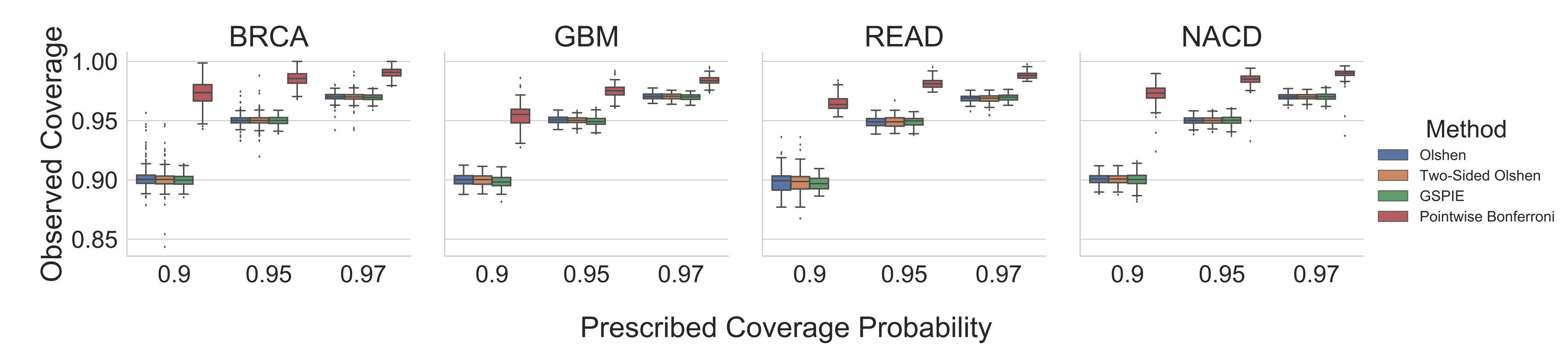 Figure 1
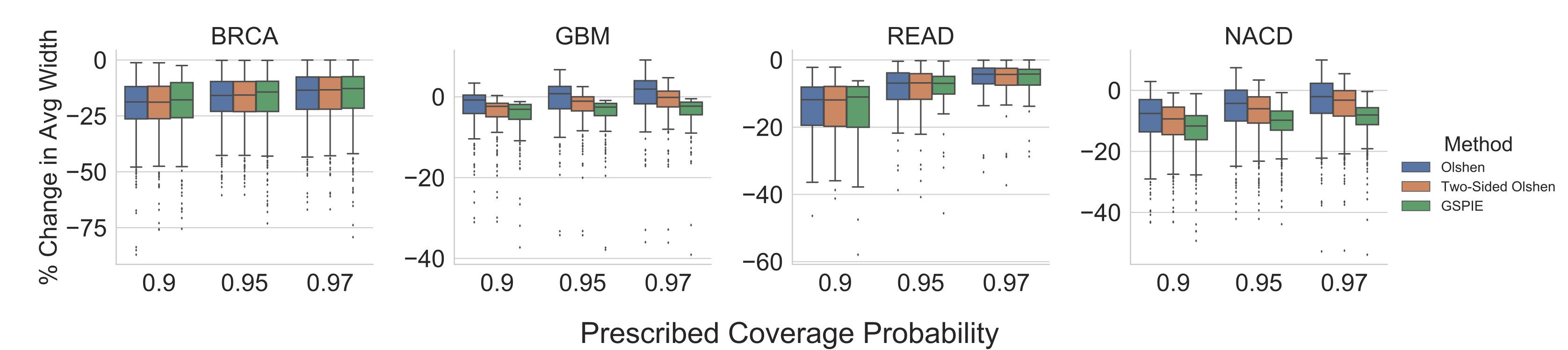 Figure 2
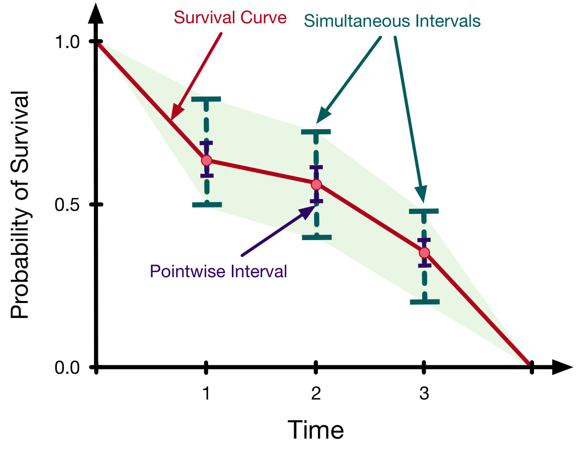 Figure 1
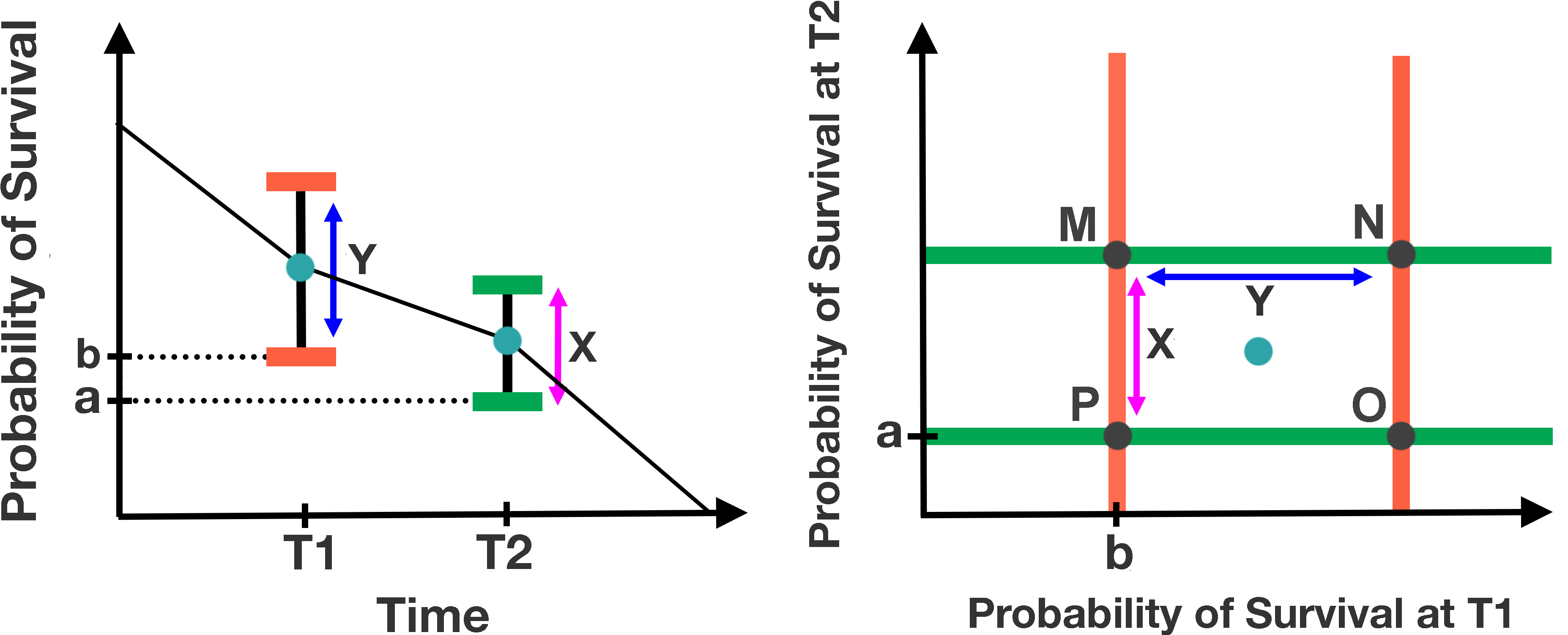 Figure 2
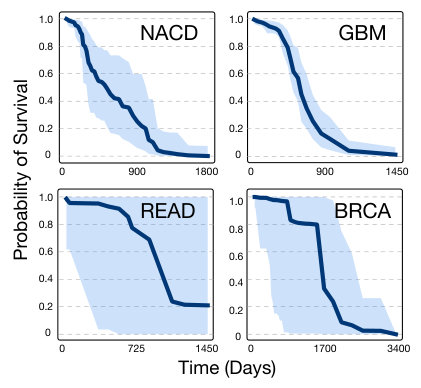 Figure 4
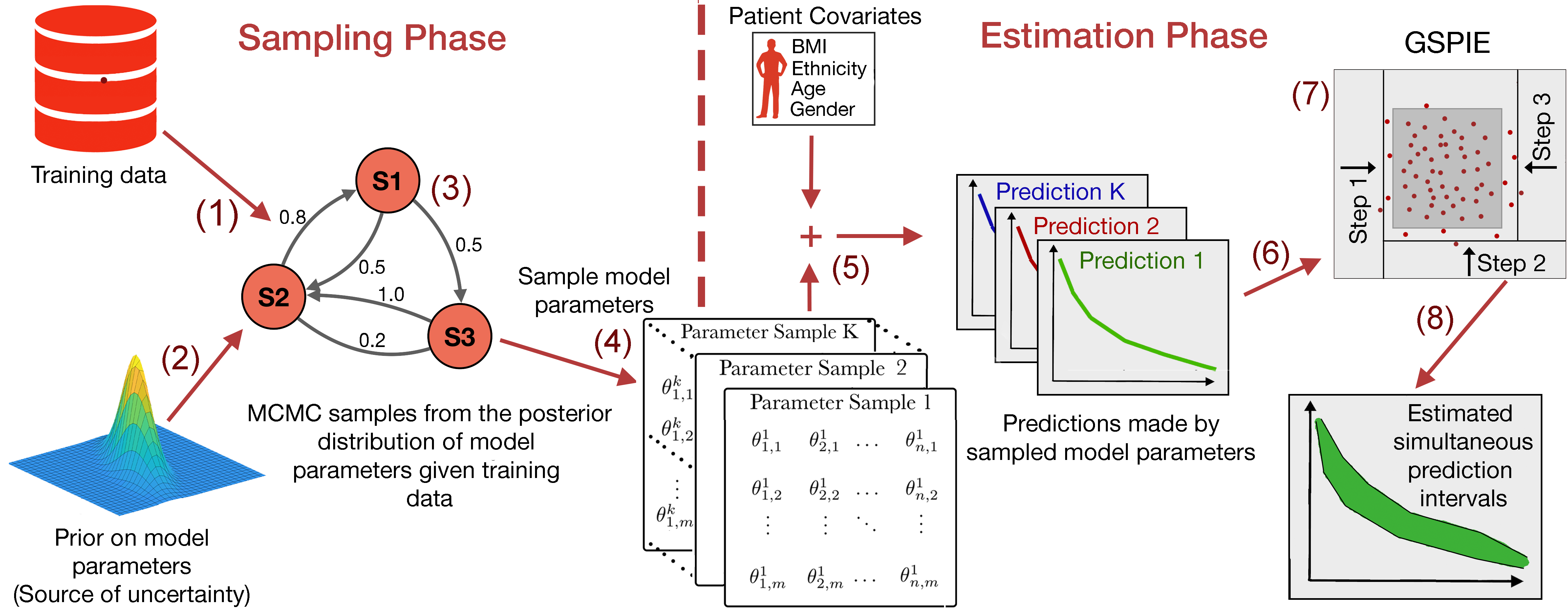 Figure 6
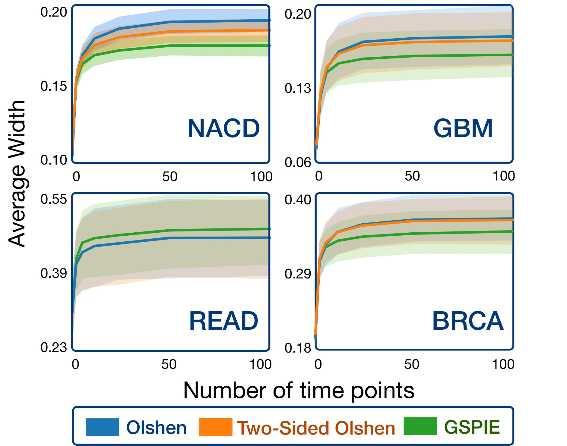 Figure 7
Peer Reviews
No public reviews on file for this paper yet. If you reviewed it on a platform where reviews are public (OpenReview, ICLR, NeurIPS, ICML), you can paste yours below so the community can read it here.
Code & Models
Videos
No videos yet. Explain this paper in a talk, walkthrough, or lecture? Add one.
Simultaneous Prediction Intervals for Patient-Specific Survival Curves
Samuel Sokota111These authors contributed equally to this work.
Ryan D’Orazio*∗*
Khurram Javed
Humza Haider
Russell Greiner
Department of Computing Science, University of Alberta {sokota, rdorazio, kjaved, hshaider, rgreiner}@ualberta.ca
Abstract
Accurate models of patient survival probabilities provide important information to clinicians prescribing care for life-threatening and terminal ailments. A recently developed class of models – known as individual survival distributions (ISDs) – produces patient-specific survival functions that offer greater descriptive power of patient outcomes than was previously possible. Unfortunately, at the time of writing, ISD models almost universally lack uncertainty quantification. In this paper we demonstrate that an existing method for estimating simultaneous prediction intervals from samples can easily be adapted for patient-specific survival curve analysis and yields accurate results. Furthermore, we introduce both a modification to the existing method and a novel method for estimating simultaneous prediction intervals and show that they offer competitive performance. It is worth emphasizing that these methods are not limited to survival analysis and can be applied in any context in which sampling the distribution of interest is tractable. Code is available at https://github.com/ssokota/spie.
1 Introduction
Understanding a patient’s probability of survival is critical for patient care – predicting survival outcomes both facilitates better treatment decisions and more informed time management. While learning survival times resembles standard regression, it is more challenging in that many training instances are censored – only a lower bound of the survival time is known. Survival analysis, a field of statistics concerned with analyzing the time until an event of interest occurs, offers a natural language for studying patient survival times. Unfortunately, most standard survival analysis tools cannot answer comprehensive questions about individual patients’ survival probabilities. Risk scores, such as those given by the Cox proportional hazards model Cox (1972), produce patient-specific hazard scores, which predict the order of patient deaths rather than survival probabilities. Single-time probabilistic models, such as the Gail model Colditz and Rosner (2000), produce a probability of survival for each patient, but only for one point in time. Population-based survival curves, such as Kaplan-Meier Kaplan and Meier (1958), offer probability values for each point in time but for populations rather than individual patients.
These limitations have motivated a class of models that learn an individual survival distribution (ISD) – a function that gives the probability that a patient with feature vector will survive to at least time Haider et al. (2018). In other words, an ISD model produces a survival curve (see Figure 1; red line) specific to each patient. This class of models includes classical systems such as the the Cox model with the Kalbfleisch-Prentice extension (Cox-KP) Kalbfleisch and Prentice (2002), and the Accelerated Failure Time model (AFT) Kalbfleisch and Prentice (2002), but also more recent models such as Random Survival Forests Ishwaran and Lu (2008), Multi-Task Logistic Regression (MTLR) Yu et al. (2011), and a host of deep learning models Luck et al. (2017); Katzman et al. (2016); Ranganath et al. (2016).
Unfortunately, while the greater complexity of ISD models allows for greater expressive power, it makes analytical uncertainty quantification difficult or impossible. This is problematic because, to make an intelligent decision based on an agglomeration of sources, it is essential that a clinician be able to understand the trustworthiness of each piece of information. If clinicians cannot judge the reliability of patient-specific survival curves, the applicability of ISD models in clinical settings is limited.
In this work we seek to remedy this situation by showcasing an easily implementable pipeline for estimating the uncertainty of patient-specific survival curves. This pipeline has two phases. First, in the sampling phase, we acquire model samples using either bootstrapping or posterior sampling. Second, in the estimation phase, we use the model samples to estimate uncertainty for specific patients. Whereas analytical methods for estimating uncertainty are typically model specific, this pipeline is largely model agnostic – it is applicable to any model for which it is feasible to acquire bootstrap or posterior samples. Many modern ISD models meet this condition and stand to benefit from the advent of flexible, efficient, and accurate uncertainty quantification.
2 Related Work
There is a large body of literature regarding the construction of confidence intervals for population-based models. The Kaplan-Meier (KM) estimator is an example of a model possessing both pointwise confidence intervals (see Figure 1; blue lines), which can be derived with Greenwood’s approximation coupled with the normal approximation Greenwood and others (1926), and confidence regions (see Figure 1; light green area), which can be derived with an adaptation of Greenwood’s formula Nair (1984) or using Brownian bridge limits Hall and Wellner (1980). Approximate confidence regions also exist for the Cox model Lin et al. (1994), and a large class of semi-parametric transform models Cheng et al. (1997) via approximations with a Gaussian process. The transformation models allow for a non-parametric baseline hazard and relax the proportional hazard assumption, making them more flexible than the Cox model. However, these transformation models assume that a predetermined function of the survival curve varies linearly with patient features. Additionally, these approximations tend to be poor at extreme time points, yielding useful confidence regions only between the smallest and largest observed event times.
Individual survival distribution models are more expressive than population-based models but in general lack uncertainty quantification. In this work we address this shortcoming by proposing a sampled-based pipeline for finding simultaneous prediction intervals over a discrete sequence of time points for patient-specific survival curves produced by ISD models. The discretization of time is less of an issue than it might seem, as many of the top performing ISD models already discretize time to facilitate learning Yu et al. (2011); Giunchiglia et al. (2018); Luck et al. (2017). Moreover, for ISD models that produce a continuous prediction, simultaneous prediction intervals can be estimated over a very large number of time points.
Closest to the present work, Olshen et al. introduced methodology to estimate simultaneous prediction intervals for gaits of normal children. The methodology, henceforth Olshen’s method, is an instance of what we refer to as a simultaneous prediction intervals estimator (SPIE). In this work we show that Olshen’s method can easily be applied to patient-specific survival analysis and offers strong performance. We also introduce both a modification to Olshen’s method and a novel SPIE which offer competitive performance.
3 Background
An ISD is a function inducing a survival curve for each patient with feature vector . In practice, many algorithms model an ISD over a discretized set of time points – i.e., each survival curve is a member of the -discretized survival space
[TABLE]
A learned ISD model of yields survival curves given by
[TABLE]
where
[TABLE]
For brevity, we will omit the superscript.
From a Bayesian perspective, has prior distribution . Because a patient’s learned survival vector is a function of , it is a random vector. This uncertainty is reflected by the predictive posterior distribution for observed training data . Usually, the posterior distribution over models does not exist in closed form. However, if the posterior can be computed up to a normalization constant – as is often the case – it can be sampled using Markov chain Monte Carlo (MCMC) methods, as is shown in the sampling phase of Figure 2. Furthermore, if the gradient of the log posterior is available, modern MCMC methods Hoffman and Gelman (2014) can efficiently sample high-dimensional parameter spaces with minimal tuning Salvatier et al. (2016). For many models, this gradient exists and can be computed with little effort using open source packages and automatic differentiation Griewank and Walther (2008).
From a frequentist perspective, uncertainty arises from the distribution over possible training datasets, each of which may induce a different instance of the model. Since the empirical distribution of data approximates the underlying distribution from which it was drawn, sampling from the empirical distribution – bootstrapping – approximates sampling possible training datasets from the underlying distribution. For models with efficient fitting procedures, an instance can be fit to each bootstrapped dataset, yielding a set of models analogous to Bayesian posterior samples collected from MCMC methods.
Ultimately, we are interested in using these sampled models to estimate simultaneous prediction intervals for the survival curves of specific patients. In the context of this work, a prediction interval is an interval within which, with a certain probability, the patient’s likelihood of survival falls at a certain time point given the observed information. Prediction intervals arise in both Bayesian and frequentist frameworks.
When dealing with -discretized survival space, we can view simultaneous prediction intervals as an orthotope222An orthotope is a Cartesian product of intervals. in . We display the visual relationship between simultaneous prediction intervals as viewed on a survival graph and as viewed as a subset of for a two-discretized survival curve in Figure 3. SPIEs can be viewed as estimating an n-dimensional orthotope that, with the prescribed probability, contains a point sampled from the appropriate n-dimensional distribution. From this perspective, given samples , Olshen’s method yields orthotopes of the form
[TABLE]
where gives the sample mean, gives the sample standard deviation, and subscript gives the th component. In our context is a set of survival curves specific to a patient with features (as shown by the green, red and blue curves in the estimation phase of Figure 2) and is the values of these survival curves at time . Ideally is chosen such that the orthotope contains a sample from the underlying distribution with probability . To approximate this choice, Olshen’s method bootstraps the samples to construct a collection of sample sets . Letting denote the proportion of elements of that are elements of , Olshen’s method chooses the smallest such that
[TABLE]
4 Methodology
The pipeline examined in this paper has two phases. In the sampling phase (see Figure 2; left) bootstrap or posterior samples of the model are acquired. These model samples approximate the uncertainty that is present in the system and are used to quantify uncertainty of predictions for new patients. In the estimation phase (see Figure 2; right), given a new patient, these model samples are used for simultaneous prediction interval estimation. In addition to investigating this framework in the context of patient-specific survival analysis, this paper also introduces two alternative SPIEs to that used by Olshen. One is a small modification to Olshen’s method that can produce asymmetric intervals; the other takes a simple but effective greedy hill climbing approach.
4.1 Two-Sided Olshen’s Method
One disadvantage of Olshen’s original method is that the prediction intervals are constrained to be symmetric about the mean. In the case of a highly asymmetric sample distribution, this could be a costly restriction. To address this, two-sided Olshen’s method replaces by , for both orthotope construction and the computation of , where is given by
[TABLE]
where gives the median, gives the sample root mean squared difference between the median and the values greater than or equal to the median, and gives the sample root mean squared difference between the median and the values less than or equal to the median. We think of and as capturing information about the variance of each side of the distribution.
4.2 Greedy Hill Climbing
A simple alternative to Olshen’s method is to do greedy optimization over the landscape of orthotopes. We call this approach greedy simultaneous prediction intervals estimator (GSPIE). GSPIE begins with an orthotope containing all samples . At each time step, GSPIE retracts one “wall” of the orthotope from its current position inwards such that it lies on the nearest sample in in the interior of (see Figure 2; (7)). GSPIE makes this decision greedily – at each time step it considers retracting each wall, selecting the retraction corresponding to the greatest reduction in interval width per sample excluded. For example, if exactly one sample lies on each wall, GSPIE takes a step that reduces the sum over interval widths of by the value
[TABLE]
where is the retraction operator discussed above moving “wall” inwards. The hill climbing procedure ends when the next retraction would leave containing less than of a validation set .
5 Experiments
In our experiments, we consider four survival datasets. The Northern Alberta Cancer Dataset (NACD; 2402 patients, 53 features, 36% censorship), includes patients with many types of cancer: including lung, colorectal, head and neck, esophagus, stomach, etc. The other three datasets are from The Cancer Genome Atlas (TCGA) Research Network Broad Institute TCGA Genome Data Analysis Center (2016): Glioblastoma multiforme (GBM; 592 patients, 12 features, 18% censorship), Rectum adenocarcinoma (READ; 170 patients, 18 features, 84% censorship), and Breast invasive carcinoma (BRCA; 1095 patients, 61 features, 86% censorship). These datasets contain “right-censored patients” – patients for whom the dataset specifies only a lower-bound on survival time.
For each dataset, we converted categorical variables into one-hot labels and imputed the mean for missing real-valued features. Each feature was normalized to mean zero and unit variance. Each dataset was shuffled and divided into a training set and a testing set with a 75/25 split. For its greedy hill climbing procedure, GSPIE divided each test patient’s survival curve samples into an optimization set and a validation set with a 50/50 split. Since our experiments are in the context of survival analysis, we project the upper and lower bounds of each estimated SPI into .
In Figure 4 we show an example of 95% simultaneous prediction intervals (with linear interpolation) of a patient’s survival function for each dataset. We attempted to select representative examples for each dataset. As might be expected, models trained on datasets with high censorship rates (READ and BRCA) yield highly uncertain survival functions.
5.1 Evaluating Performance
In evaluating SPIEs, there are two metrics of concern. First, an estimator should be accurate – prescribing a coverage probability should yield simultaneous intervals that include a random sample with probability . Second, an estimator should produce tight prediction intervals – i.e., simultaneous prediction intervals with small average width. However, note that these two metrics are not independently meaningful. It is neither useful to have loose, accurate intervals, nor to have tight inaccurate intervals.333Though in many contexts we may not mind a method producing conservative simultaneous intervals, insofar as conservatism does not come at the cost of tightness. Unfortunately, as far we are aware, there exists no established metric that unifies accuracy and tightness in a manner that is robust to different tradeoff preferences. Therefore, while we present these metrics separately, we encourage readers to take a holistic perspective.
To examine the performance of these methods, we used multi-task logistic regression (MTLR), which had the strongest performance of the methods examined in Haider et al. (2018), as our ISD model. We trained MTLR using a regularization factor of 1/2, which was tuned with five-fold cross-validation and time points (where is the size of the training set), such that an equal number of events occurs between each two time points, as is recommended by Yu et al. (2011). We considered a Bayesian approach – we collected 10,000 posterior samples from the posterior using NUTS Hoffman and Gelman (2014) and estimated joint prediction intervals for the predictive posterior distribution of test set patients. We used an isotropic Gaussian prior for MTLR’s model parameters with a variance corresponding with the tuned regularization factor. While not strictly necessary, enforcing this correspondence causes the predictions from the fitted MTLR model to coincide with the maximum a posteriori (MAP) estimate.
5.1.1 Accuracy
To evaluate the accuracy of the prediction orthotopes, we ran a second chain and collected 10,000 test samples from the predictive posterior distribution for each test set patient. Accurate simultaneous prediction intervals should contain roughly of these samples. Figure 5 displays the results of the analysis on each patient in the test set. We include Olshen’s method, two-sided Olshen’s method, GSPIE, and also a pointwise interval baseline444Pointwise intervals were obtained from percentile estimates via the ogive (i.e., the empirical distribution with linear interpolation). with a Bonferroni correction. The most significant takeaway from the results is that the former three methods are much more accurate than the conservative Bonferroni correction, which guarantees a lower bound on the coverage probability of the simultaneous intervals. Of course, the accuracy of all of the methods is highly dependent on the number of model samples that are available.
5.1.2 Tightness
To evaluate the tightness of the prediction intervals we measure the average interval width. On a survival graph, this metric is proportional to Lebesgue measure in the case that intervals exist for every time point, but extends more sensibly to our circumstance, in which intervals exist for only a finite number of time points. Figure 6 displays the result of the analysis. For each patient in the test set and for each SPIE, we measured the percentage change in the average interval width compared to pointwise intervals with a Bonferroni correction – lower is better. For BRCA and READ, all three methods appear to have perform similarly, notably exceeding the baseline. For GBM and NACD, there seems to be a clearer distinction between the methods – GSPIE generally gave tighter intervals than two-sided Olshen’s method, which itself generally gave tighter intervals than Olshen’s method.
5.2 Discretization of Continuous Time Curves
Although the methods discussed in this paper are limited to a finite number of time points, there is no reason they cannot be applied to ISD models that produce continuous time curves. However, one might worry that using a very large number of time points (i.e., a fine discretization) might cause SPIEs to produce trivially large prediction intervals. To investigate this possibility, we used the Weibull accelerated failure time model Kalbfleisch and Prentice (2002), which produces continuous time patient-specific survival curves, on each of the four datasets. We considered a Bayesian perspective, assuming an isotropic Gaussian prior for the model parameters and a Gumbel distribution with a half-normal hyperprior for the noise. We show the results in Figure 7, where mean average width with 95% pointwise confidence intervals is plotted as a function of the discretization for each of the different datasets. We observe that all three methods were able to find highly nontrivial simultaneous prediction intervals for finely discretized curves. We expect this result to hold generally across other continuous models and datasets.
5.3 Discussion
Our experiments suggest that Olshen’s method, two-sided Olshen’s method, and GSPIE all perform well as SPIEs. All three are accurate, efficient, find relatively tight intervals, and can be applied to continuous time models with fine discretizations. The right choice of estimator appears to be context dependent. For example, with MTLR, on NACD and GBM, GSPIE may offer the best compromise between accuracy and tightness, whereas on READ and BRCA, it is less clear. Luckily, given that all three methods are efficient and can make use of the same model samples, it is relatively easy to try and test555One can simply take more model samples to verify that estimated intervals meet their prescription, as was done in our experiments. all of them.
6 Conclusion
In this work we promote a framework for quantifying the uncertainty of patient-specific survival curves. The methods examined here are easily-implementable and applicable to a large class of ISD models. We hope this framework will allow clinicians to more comfortably consider ISD models as a source of information for patient-specific decisions.
Lastly, although the focus of this paper is patient-specific survival analysis, the SPIEs we examined are general purpose tools for estimating SPI from samples. We anticipate that these methods could prove useful in many contexts outside of survival analysis, such as time series analysis, trigonometric regression, and quantile regression.
The reference list from the paper itself. Each links out to its DOI / PubMed record.
- 1Broad Institute TCGA Genome Data Analysis Center (2016) Broad Institute TCGA Genome Data Analysis Center. Analysis-ready standardized tcga data from broad gdac firehose 2016_01_28 run, 2016.
- 2Cheng et al. (1997) SC Cheng, LJ Wei, and Z Ying. Predicting survival probabilities with semiparametric transformation models. Journal of the American Statistical Association , 1997.
- 3Colditz and Rosner (2000) Graham A. Colditz and Bernard A Rosner. Cumulative risk of breast cancer to age 70 years according to risk factor status: data from the nurses’ health study. American journal of epidemiology , 2000.
- 4Cox (1972) David R Cox. Regression models and life-tables. Journal of the Royal Statistical Society: Series B (Methodological) , 34(2):187–202, 1972.
- 5Giunchiglia et al. (2018) Eleonora Giunchiglia, Anton Nemchenko, and Mihaela van der Schaar. Rnn-surv: A deep recurrent model for survival analysis. In International Conference on Artificial Neural Networks . Springer, 2018.
- 6Greenwood and others (1926) Major Greenwood et al. A report on the natural duration of cancer. A Report on the Natural Duration of Cancer. , 1926.
- 7Griewank and Walther (2008) Andreas Griewank and Andrea Walther. Evaluating derivatives: principles and techniques of algorithmic differentiation , volume 105. Siam, 2008.
- 8Haider et al. (2018) Humza Haider, Bret Hoehn, Sarah Davis, and Russell Greiner. Effective ways to build and evaluate individual survival distributions. ar Xiv:1811.11347 , 2018.
