Construction of anti-de Sitter-like spacetimes using the metric conformal Einstein field equations: the tracefree matter case
Diego A. Carranza, Juan A. Valiente Kroon

TL;DR
This paper develops a method to construct anti-de Sitter-like spacetimes with tracefree matter using conformal Einstein equations, ensuring local existence and uniqueness of solutions through a wave equation approach.
Contribution
It introduces a systematic procedure for initial-boundary value problems in conformal Einstein equations with tracefree matter, including explicit models like scalar, Maxwell, and Yang-Mills fields.
Findings
Established local existence and uniqueness of solutions.
Analyzed conformal constraints for initial and boundary data.
Identified data requirements for coupling matter models.
Abstract
Using a metric conformal formulation of the Einstein equations, we develop a construction of 4-dimensional anti-de Sitter-like spacetimes coupled to tracefree matter models. Our strategy relies on the formulation of an initial-boundary problem for a system of quasilinear wave equations for various conformal fields by exploiting the conformal and coordinate gauges. By analysing the conformal constraints we show a systematic procedure to prescribe initial and boundary data. This analysis is complemented by the propagation of the constraints, showing that a solution to the wave equations implies a solution to the Einstein field equations. In addition, we study three explicit tracefree matter models: the conformally invariant scalar field, the Maxwell field and the Yang-Mills field. For each one of these we identify the basic data required to couple them to the system of wave equations. As…
Click any figure to enlarge with its caption.
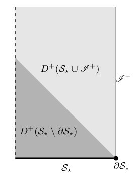 Figure 1
Peer Reviews
No public reviews on file for this paper yet. If you reviewed it on a platform where reviews are public (OpenReview, ICLR, NeurIPS, ICML), you can paste yours below so the community can read it here.
Videos
No videos yet. Explain this paper in a talk, walkthrough, or lecture? Add one.
Construction of anti-de Sitter-like spacetimes using the metric
conformal Einstein field equations: the tracefree matter case
Diego A. Carranza111E-mail address:[email protected]
School of Mathematical Sciences, Queen Mary University of London, Mile End Road, London E1 4NS, United Kingdom.
Juan A. Valiente Kroon222E-mail address:[email protected]
School of Mathematical Sciences, Queen Mary University of London, Mile End Road, London E1 4NS, United Kingdom.
Abstract
Using a metric conformal formulation of the Einstein equations, we develop a construction of 4-dimensional anti-de Sitter-like spacetimes coupled to tracefree matter models. Our strategy relies on the formulation of an initial-boundary problem for a system of quasilinear wave equations for various conformal fields by exploiting the conformal and coordinate gauges. By analysing the conformal constraints we show a systematic procedure to prescribe initial and boundary data. This analysis is complemented by the propagation of the constraints, showing that a solution to the wave equations implies a solution to the Einstein field equations. In addition, we study three explicit tracefree matter models: the conformally invariant scalar field, the Maxwell field and the Yang-Mills field. For each one of these we identify the basic data required to couple them to the system of wave equations. As our main result, we establish the local existence and uniqueness of solutions for the evolution system in a neighbourhood around the corner, provided compatibility conditions for the initial and boundary data are imposed up to a certain order.
1 Introduction
The study of solutions to the Einstein equations with negative Cosmological constant, the so-called anti-de Sitter-like spacetimes, results particularly challenging due to the presence of a timelike conformal boundary located at spatial infinity. This boundary makes the spacetime non-globally hyperbolic and, thus, it cannot be fully reconstructed from an initial value problem. Accordingly, information on the conformal boundary must also be provided. In this scenario, the methods of conformal geometry offer a natural approach to face this challenge by providing an (unphysical) auxiliary spacetime where the boundary is located at a finite distance.
Although the use of conformal methods into General Relativity can be traced back to Penrose’s seminal work [27], a satisfactory conformal formulation of the Einstein field equations from the point of view of the theory of partial differential equations was first obtained by Friedrich [15]. The latter enabled a systematic study of asymptotically simple solutions to Einstein equations. In particular, it made possible a construction of vacuum anti-de Sitter-like spacetimes where a non-metric formulation of conformal Einstein field equations is employed [18, 19]. At the heart of this approach is a first order symmetric hyperbolic system for a set of conformal fields obtained by exploiting the properties of certain conformal invariants —the so-called conformal geodesics. For this evolution system, maximally dissipative boundary conditions are considered in order to establish a result of local existence of solutions. Despite identifying some boundary data in a covariant manner, the type of equations used in this construction, in conjunction with the gauge choice, makes it difficult to implement this scheme in numerical codes.
The latter issue becomes particularly relevant in view of the growing interest in the conjectured instability of the anti-de Sitter spacetime —see [5] for an entry point into the subject. A considerable amount of effort has been directed to understand the dynamics of this class of solutions via numerical methods —see, for example, [4, 6, 14, 13, 1, 11]. Also, alternative hyperbolic formulations coupling the scalar field have been discussed in [28, 29] and a proof of this conjecture has been obtained for the Einstein-Vlasov system with spherical symmetry [25].
As an alternative to solving first order systems, Paetz [26] showed that, in the vacuum case, it is possible to construct a second order evolution system from the conformal Einstein equations. Based on this result, in [7] an alternative construction for vacuum anti-de Sitter-like spacetimes has recently been given. Using a metric version of the conformal Einstein fields equations, a suitable choice of coordinates makes it possible to obtain a quasilinear system of wave equations for a set of conformal fields. Moreover, the identified free boundary data consist of a Lorentzian 3-metric on this hypersurface together with a linear combination of the incoming and outgoing gravitational radiation. Due to the manifestly hyperbolic nature of the system under consideration, it is expected that this scheme can be more easily adapted to current numerical codes.
The study of the Einstein field equations coupled to some suitable matter model is generally carried out on a case-by-case manner. Remarkably, in the context of conformal methods, tracefree matter models are amenable to a more systematic study. This class of matter models contains several cases of interest such as the electromagnetic and Yang-Mills fields. In [17], Friedrich has provided a suitable conformal formulation of the Einstein field equations under the assumption of a tracefree energy-momentum tensor, which, in turn, has been exploited to establish stability results for the Einstein-Yang-Mills system with positive and zero Cosmological constant. Motivated by this investigation, a local existence and uniqueness result for the same system has been presented in [24] under the assumption of spherical symmetry. Despite the complications from considering non-trivial matter fields, advances have been made in a variety of scenarios using different approaches —see, for example, [22, 20, 21]. Nevertheless, a satisfactory conformal formulation allowing a methodical study of general matter models remains elusive.
In the present article we generalise the analysis in [7] and consider the construction of anti-de Sitter-like spacetimes coupled to tracefree matter models. Exploiting the conformal freedom we set an appropriate gauge yielding a system of geometric wave equations for the relevant conformal fields [8]. A suitable coordinate choice allows us to cast it as a system of quasilinear of wave equations, provided the matter field has good properties. For this type of hyperbolic evolution equations there are available results concerning the local existence and uniqueness of solutions —see e.g. [9, 12]. The conformal constraints supply the system with adequate initial and boundary data. In this work three models of tracefree matter are considered: the conformally invariant scalar field, the Maxwell field and the Yang-Mills field. Initial and boundary data have been identified for each one of them, as well as an analysis of the corresponding propagation of the constraints. Given the amount of heavy calculations some parts of this work require, the suite xAct of Mathematica for tensorial computations has been employed —see [31].
The main result of the article can be stated as follows:
Theorem 1**.**
Let be a 3-dimensional spacelike hypersurface with boundary and on it smooth tracefree anti-de Sitter-like initial data for the Einstein field equations coupled to either: (i) the conformally invariant scalar field, (ii) the Maxwell field or (iii) the Yang-Mills field. Consider the cylinder for some endowed with a set of smooth fields satisfying the conformal Einstein constraints on . Assume suitable basic boundary data for the tracefree matter fields. If, in addition, the data on and on satisfy, up to some order, compatibility (i.e. corner) conditions at , then there exists a smooth solution to the Einstein field equations with coupled to any of the aforementioned tracefree matter fields in a neighbourhood of .
The proof of this theorem follows from the analysis of the various sections of the article. The detailed boundary conditions for the geometric fields are detailed in Proposition 4 while those for the matter fields are detailed in Lemmas 5, 6 and 7. To the best of our knowledge, the results in Theorem 1 are the first results regarding the local existence of non-vacuum anti-de Sitter-like spacetimes in the absence of symmetries available in the literature.
1.1 Outline of the article
This article builds on the theory developed in [7] and [8]. In order to ease the presentation we make direct use of the relevant results of these references and refer the reader to them for full details. Accordingly, in this article we emphasise the novel aspects of the analysis and how the ideas of the above references fit together.
In Section 2 the basic definitions related to the conformal formulation of the Einstein equations used throughout this work are introduced. Section 3 is devoted to the discussion of the evolution system for the conformal fields and the role the gauge choice plays in its successful recasting as a hyperbolic system; also, the set of zero-quantities are defined. Section 4 presents some results about the conformal constraint equations on spacelike and timelike hypersurfaces. In Section 5 we focus on analysing the boundary data required to establish a well-posed problem for the system of wave equations and their relation to the zero-quantities. In Section 6 we provide a brief discussion of how the boundary data enables us to propagate the constraints on the conformal boundary. In Section 7 several explicit matter models are studied in detail, focusing on the basic data necessary to couple them to the evolution system. Finally, Section 8 provides some final remarks.
Conventions
Throughout this work, will denote a 4-dimensional Lorentzian spacetime satisfying the Einstein equations with Cosmological constant . The signature of the metric in this article will be . Lowercase Latin letters are used as abstract spacetime tensor indices while the indices are abstract indices on the tensor bundle of hypersurfaces of . Greek letters will be used as coordinate indices on either spacelike or timelike hypersurfaces. Our conventions for the curvature are
[TABLE]
2 The tracefree metric conformal Einstein field equations
This section discusses some properties of the tracefree conformal Einstein field equations, the basic tool to be used in the remainder of this article. The system of geometric wave equations resulting from the conformal Einstein field equations is briefly analysed. Finally, it is also discussed how a suitable gauge choice enables us to cast these evolution equations as a quasilinear hyperbolic system.
2.1 Basic definitions
Let denote a physical spacetime satisfying the Einstein field equations
[TABLE]
where is the Ricci tensor of the metric , the energy-momentum tensor and its trace. Let be a spacetime conformally related to via a conformal embedding
[TABLE]
with the so-called conformal factor. Abusing of the notation we write
[TABLE]
We will refer to as the unphysical spacetime. The set of points of for which vanishes define the conformal boundary. We use the notation to denote the parts of the conformal boundary which are a hypersurface of .
In what follows let and denote, respectively, the Riemann tensor, the Ricci tensor, the Ricci scalar and the (conformally invariant) Weyl tensor of the metric . For the discussion of the metric conformal Einstein field equations we conveniently introduce the fields
[TABLE]
known, respectively, as the Schouten tensor, the Friedrich scalar and the rescaled Weyl tensor.
2.2 The energy-momentum tensor
Unlike the various geometrical objects associated to the metric , the rescaling (2) does not determine the transformation rule for the energy-momentum tensor. Then, for simplicity, let define its unphysical counterpart as
[TABLE]
In terms of the Levi-Civita connection of the unphysical metric , this rescaling implies that
[TABLE]
where it has been used that is divergencefree and . From here we have that
[TABLE]
Remark 1**.**
From equation (4) it can be checked that if . In view of this it will be assumed hereafter that the physical matter model is tracefree.**
Due to the presence of a non-vanishing tracefree matter component it results convenient to introduce the rescaled Cotton tensor
[TABLE]
From this definition it follows that it possesses the symmetries and .
2.3 Basic properties
In terms of the objects defined above, the tracefree metric conformal Einstein field equations are given by [17]:
[TABLE]
A detailed derivation and discussion of this system of equations can be found in [30]. Additionally, as a consequence of imposing the tracefree condition on the matter sector, the system is supplemented by the conservation law
[TABLE]
Remark 2**.**
Equations (6a)-(6d) are read as differential conditions for the fields and subject to the condition . Equation (6e) plays the role of an algebraic constraint which is satisfied if it holds at a single point by virtue of the other equations —see Lemma 8.1 in [30]. Equation (6f) establishes the irreducible decomposition of the Riemann tensor. Moreover, it also provides an equation for .**
Remark 3**.**
Direct evaluation of (6e) on the conformal boundary shows that the causal character of is completely determined by the sign of the Cosmological constant . In particular, for anti de Sitter-like spacetimes () is timelike —see e.g. Theorem 10.1 in [30].**
By a solution to the tracefree metric conformal Einstein field equations it is understood a collection satisfying equations (6a)-(6e) and (7). The relation between the metric conformal Einstein field equations and the Einstein field equations is given by the following statement:
Proposition 1**.**
Let denote a solution to the metric tracefree conformal Einstein field equations such that on an open set . If, in addition, equation (6e) is satisfied at a point , then the metric
[TABLE]
is a solution to the Einstein field equations (1) on .
A proof of this proposition is given in [30] —see Proposition 8.1.
3 The evolution system
In [26] Paetz has proved that if it is possible to obtain a system of geometric wave equations for the collection of conformal fields . This has been generalised to the tracefree matter case in [8], resulting in the following:
Proposition 2**.**
Any solution to the tracefree metric conformal Einstein field equations (6a)-(6d) satisfies the equations
[TABLE]
Remark 4**.**
The system (8a)-(8d) needs to be supplemented with a wave equation for the unphysical metric. Taking the trace of (6f) we obtain
[TABLE]
Here, encodes the derivatives of once a system of coordinates has been adopted, while is an independent field satisfying the system (8a)-(8d). The last equation can be viewed as an Einstein field equation for coupled to some unphysical matter fields. In view of this, equation (9) be known as the unphysical Einstein equation.**
Remark 5**.**
Equations (8a)-(8d) and (9) are not completely satisfactory wave equations for a number of reasons: (i) the appearance of second order derivatives of ; (ii) once coordinates are introduced, undesired second order derivatives of the components of appear in the principal part of equations (8c), (8d) and (9); (iii) when a particular matter model is considered, second (and higher) order derivatives of the corresponding field will emerge in the coupled system. In order to apply results from the theory of partial differential equations, these problems must be addressed. Issues (i) and (ii) have been discussed in [7] and will be briefly presented in the next subsection, while (iii) has been analysed in [8] for some particular models.**
3.1 Gauge considerations
The conformal Einstein field equations possess both a coordinate and a conformal freedom which can be exploited to recast the geometric wave equations (8a)-(8d) as satisfactory hyperbolic evolution equations. This subsection is based on [7], Section 2.3, where a more detailed presentation and the motivation behind the relevant definitions can be found.
3.1.1 Conformal gauge source function
Given two conformally related metrics and , the relation between their corresponding Ricci scalars can be read as a differential equation for their conformal factor . Then, prescribing the Ricci scalar is equivalent to the specification of the representative of the conformal class . Accordingly, the Ricci scalar associated to the unphysical metric will be specified by the gauge function —that is
[TABLE]
3.1.2 Generalised harmonic coordinates and the reduced Ricci operator
The other piece of the gauge freedom is contained in the coordinate choice. Let be coordinates satisfying the generalised wave condition
[TABLE]
where are the so-called coordinate gauge source functions. A simple calculation shows that these are related to the contracted Christoffel symbols via
[TABLE]
In this context, we introduced the reduced Ricci operator
[TABLE]
Here, is given explicitly in terms of first and second order partial derivatives of . Thus, by choosing coordinates satisfying condition (10), the unphysical Einstein equations (9) takes the form
[TABLE]
By choosing generalised wave coordinates, this equation does correspond to a quasilinear wave equation for the components of .
3.1.3 The reduced wave operator
As remarked before, when the operator for an arbitrary coordinates choice is applied on a tensorial field, undesired second derivatives of appear. In this sense this operator is not suitable if one wants to preserve the hyperbolicity of the system. Making use of the generalised wave coordinate condition, a suitable operator can be defined as follows:
Definition 1**.**
Let be a tensor field. The action of the reduced wave operator, , on it is given by:
[TABLE]
where . The action of on a scalar field is simply given by
[TABLE]
As shown in [7], if generalised wave coordinates are chosen then represents a suitable second order hyperbolic operator for the system (8a)-(8d). In this sense, we will say that a system of wave equations expressed in terms of is proper.
3.1.4 Summary: gauge reduced evolution equations
In view of the previous discussion, and as presented in [8], when generalised wave coordinates are adopted, the system of wave equations for the components of the conformal geometric fields to be considered is the following:
[TABLE]
Remark 6**.**
Since the operator enables us to remove all the undesired second order partial derivatives of , the reduced system (13a)-(13e) constitutes a system of quasilinear wave equations for the fields , , , and . Strictly speaking though, this is a system of wave equations only if is known to be Lorentzian. Precise statements concerning the local existence and uniqueness results for this type of systems can be found in [9, 12].**
Remark 7**.**
One has to prove that the gauge introduced in this section is consistent with the field equations. In [8] it has been shown how to construct a system of homogeneous wave equations for an additional set of subsidiary fields under the assumption of a tracefree energy-momentum tensor. The conditions required to establish vanishing initial and boundary data for these fields have been described in [7], from where the propagation of the gauge follows.**
3.2 The subsidiary evolution equations
Once a suitable system of wave equations for the conformal fields has been obtained, it is necessary to prove that any solution to this system corresponds to a solution to the metric tracefree conformal Einstein field equations (6a)-(6d). This can be achieved by first defining the set of geometric zero-quantities
[TABLE]
In terms of these fields, the metric tracefree conformal Einstein field equations can be expressed as
[TABLE]
In [8] it has been shown that the evolution of these quantities can be encoded in a system of homogeneous geometric wave equations. This result can be enunciated as follows:
Lemma 1**.**
Assume that the conformal fields , , and satisfy the geometric wave equations (8a)-(8d). Then the geometric zero-quantities satisfy a system of geometric wave equations of the form
[TABLE]
where , , , , and are homogeneous expressions of their arguments.
Remark 8**.**
In order to cast equations (16a)-(16f) as a proper quasilinear system of wave equations, the operator must be replaced by the reduced wave operator once generalised wave coordinates have been chosen.**
4 The conformal constraint equations
This section will be devoted to the discussion of the constraint equations implied by the metric tracefree conformal Einstein field equations. This system, first discussed in [16], will serve to construct the initial and boundary data sets required to establish a well-posed initial-boundary problem for the wave equations (13a)-(13e). A detailed discussion of their derivation and properties in the general matter case can be found in [30], Chapter 11.
4.1 Basic definitions
Let denote a (spacelike or timelike) hypersurface of the unphysical spacetime with unit normal vector . Then, we define the norm of as:
[TABLE]
so that take the values 1 or -1 for timelike or spacelike hypersurfaces , respectively. The normal vector induces a decomposition via the projector to
[TABLE]
The intrinsic derivative on is defined in the following way: let be a scalar function and be a tensor field on , then
[TABLE]
Expressions involving higher rank tensors follow an analogous rule. The derivative in the direction of (simply called the normal derivative) is given by
[TABLE]
The extrinsic curvature of is defined as
[TABLE]
In the following let
[TABLE]
denote, respectively, the pull-backs of the following geometric objects
[TABLE]
to . In order to take into account the contributions from the matter fields, let and stand, respectively, for the pull-backs of the projections
[TABLE]
Remark 9**.**
The tensor corresponds to the 3-metric induced by on and it will be either Lorentzian if is timelike or Riemannian if it is spacelike. Similarly, we will denote by the pull-back of and by its trace.**
Remark 10**.**
The fields and encode, respectively, the electric and magnetic parts of the rescaled Weyl tensor with respect to the normal . It can be verified that
[TABLE]
From this point onwards, the restriction of the conformal factor to the conformal boundary will be denoted by —that is,
[TABLE]
Next, we define the Schouten tensor of the intrinsic 3-metric ,
[TABLE]
where and are the corresponding intrinsic Ricci tensor and scalar. In terms of these fields, a number of constraints are obtained from the different projections of equations (6a)-(6e) to . This results in the intrinsic equations
[TABLE]
This system is supplemented by two geometric constraints arising from (6f), namely, the conformal Codazzi-Mainardi and Gauss-Codazzi equations:
[TABLE]
Relations (17a)-(17h), (18a) and (18b) are called the metric tracefree conformal constraint equations. A full derivation of this system can be found in [30] along with an extensive discussion of their properties.
4.1.1 The conformal constraints on the conformal boundary
Let be the intrinsic Lorentzian 3-metric associated to the conformal boundary with normal vector . In the following, objects and operators crossed by a line will represent projections obtained via and . Also, will denote an equality valid on . Evaluating the conformal constraints on the conformal boundary () we obtain the following simplified system:
[TABLE]
A procedure to solve these equations in the vacuum case has been discussed in [18] where the solution is given in terms of a gauge quantity related to the Friedrich scalar and the rescaled Cotton tensor of . The latter is defined as
[TABLE]
Adopting this approach, the following result can be enunciated:
Proposition 3**.**
Let be a 4-dimensional manifold and a timelike conformal boundary with intrinsic 3-dimensional Lorentzian metric and normal . Consider a tracefree energy-momentum tensor with its orthogonal-normal projection with respect to . Let be a smooth scalar gauge function defined on . Then a solution to the tracefree conformal constraint equations (19a)-(19j) on is given by the fields
[TABLE]
along with a tracefree symmetric tensor field satisfying
[TABLE]
Proof.
Firstly, is given by (19h). As mentioned before, is a gauge quantity on and expressed by equation . Direct substitution into constraints (19a), (19c), (19j) and (19d) readily leads to the solutions for and , respectively. Using these, equations (19b), (19e) and (19i) are trivially satisfied. Regarding the equations with matter terms, when the fields and are written explicitly in terms of the energy-momentum tensor via equation (5), a straightforward calculation yields
[TABLE]
On the other hand, by virtue of the definition of , it follows that that . Using this and the expressions for and stated above, it is found that (19f) is trivially satisfied and (19g) corresponds to equation (21). ∎
Having obtained the solutions for the constraint equations on the conformal boundary, a converse-like result can be formulated with the addition of an auxiliary assumption:
Lemma 2**.**
Let be a timelike hypersurface such that conditions (20a)-(20e) hold. If on some fiduciary spacelike hypersurface of , then one has that on
Proof.
Consider the case when on . Using equations (20b), (20c) and (20e), the trace of the conformal constraint (17a) provides with the following wave equation for to be satisfied on :
[TABLE]
where it has been used that for a tracefree unphysical energy-momentum tensor . On the other hand, when (20a), (20c) and are substituted into constraint we have
[TABLE]
As and on , it follows from the last equation that on , which represents a first order initial condition for . Due to the homogeneity of (22), along with the uniqueness of its solutions, we conclude then that on , that is to say, it corresponds to the conformal boundary. Regarding the case , it has been showed in [7] how the conformal gauge freedom can be exploited to render this case into the one. ∎
4.1.2 Solutions to the conformal constraints on a spacelike hypersurface
Constraint equations (17a)-(18b) enable us to obtain the conformal version of the so-called Hamiltonian and Momentum constraints on a spacelike hypersurface . A straightforward calculation shows that for a tracefree matter field these take the form:
[TABLE]
It follows that under a conformal approach, the collection of fields satisfying the previous equations must be prescribed as the basic initial data, i.e. they determine the remaining fields on a spacelike hypersurface. Together with the boundary data, this set will serve to evolve the wave equations for the conformal fields. Directly from the conformal constraints one obtains the following expressions for the initial data:
[TABLE]
The fact that these expressions are singular at leads to the following:
Definition 2** **(**anti-de Sitter-like initial data with
tracefree matter**).
For a tracefree anti-de Sitter-like initial data set it is understood a 3-manifold with boundary together with a collection of smooth fields such that:
- (i)
* on ;*
- (ii)
* and on ;*
- (iii)
the fields , , , and computed from relations (25a)-(25e) extend smoothly to .
Remark 11**.**
Anti-de Sitter-like initial data sets are closely related to so-called hyperboloidal data sets for Minkowski-like spacetimes —see [23]. By means of this correspondence it is possible to adapt the existence results for hyperboloidal initial data sets in [2, 3] to the anti-de Sitter-like setting. In particular, this shows the existence of a large class of time symmetric data, i.e. data for which .**
5 General set-up
In this section we identify the relevant boundary data required for the formulation of the initial-boundary problem for anti-de Sitter-like spacetimes with tracefree matter. Except for the data corresponding to the electric part of the Weyl tensor, the rest of the construction is identical to the one for the vacuum case analysed in [7] where a more detailed discussion is presented.
Let be a conformal extension of an anti-de Sitter-like spacetime where and are conformally related metrics. Let be a smooth, compact and oriented spacelike hypersurface with boundary . Furthermore, is the so-called corner. The portion of in the future of will be denoted by . In addition, it will be assumed that the causal future coincides with the future domain of dependence and that so that, in particular, —see Figure 1.
5.1 Coordinates
Let us introduce adapted coordinates such that and are given as
[TABLE]
so the corner is defined by the condition . Coordinates are propagated off via the generalised wave coordinated condition (10). Observe that this can always be locally solved: the expression above provides the value of the coordinates on while their normal derivatives are obtained from the coordinates are are independent, that is to say, the coordinate differentials must be linearly independent.
5.2 Boundary conditions for the conformal evolution equations
In order to formulate an initial-boundary problem for anti-de Sitter-like spacetimes we must provide Dirichlet boundary data for the wave equations (13a)-(13e) on the conformal boundary. Next we summarise the results found in [7] which directly extend to the tracefree case.
Adopting a Gaussian gauge on the conformal boundary, the metric can be written as
[TABLE]
with the components of the Lorentzian 3-metric . In terms of this the boundary data are
[TABLE]
where is given by . However, the data for the electric part of the Weyl tensor differs from the one in the vacuum case, so it will be analysed in the next subsection.
5.2.1 Boundary data for
As showed in Proposition 3, the electric part of the rescaled Weyl tensor is determined by equation (21). In order to analyse this differential equation it is convenient to perform a decomposition on the conformal boundary. For this purpose consider a foliation of given by a family of spacelike hypersurfaces with normal vector . This induces the projector
[TABLE]
In an analogous manner to Section 4, we define the intrinsic derivative operator satisfying along with a normal derivative . The projector allows us to further decompose tensors and with respect to as
[TABLE]
where the different components are defined as:
[TABLE]
From this it follows that . Assuming that the acceleration locally vanishes, we introduce the extrinsic curvature associated to the foliation, as well as its trace . A calculation shows that equation (21) implies the system
[TABLE]
with being the -tracefree part of .
Remark 12**.**
If and are given, then equations (26a)-(26b) constitute a symmetric hyperbolic system for and . In this sense, these fields constitute additional pieces of basic boundary data. The particular tracefree matter model in consideration will determine and in an explicit way. On the other hand, as noticed in [7], the two independent components of can be related to the notions of incoming and outgoing radiation. By exploiting the Newman-Penrose formalism, this can be expressed in terms of two complex-valued scalar fields and .
The above discussion leads to:
Lemma 3**.**
Let be endowed with the following smooth fields:
- (i)
a 3-dimensional Lorentzian metric ;
- (ii)
a set of coordinate gauge source functions and the gauge function ;
- (iii)
a symmetric tensor which is spatial with respect to the foliation induced on by the functions and tracefree with respect to the metric induced on the leaves of the foliation;
- (iv)
a spatial (in the same sense as in (iii)) vector , and scalars and ;
- (v)
a choice of fields and on a fiduciary hypersurface of .
Then there exists such that on the cylinder the fields and are uniquely determined and, together with the fields prescribed in (iii) and (iv), satisfy the constraint (21).
5.3 Summary
The analysis of this section can be summarised in the following:
Proposition 4**.**
Let be a collection of smooth fields defined on as in Lemma 3 and be the fields constructed according to the procedure described in the previous subsection. Then, the zero-quantities defined by relations (14a)-(14f) satisfy
[TABLE]
at least on .
Remark 13**.**
Notice that the boundary data discussed throughout this section is not necessarily consistent with the initial data at the corner. Demanding the compatibility of these two sets of data requires to impose so-called corner conditions. If one considers asymptotically hyperbolic initial data, a gluing construction allows to satisfy these conditions to any arbitrary order [10]. In the present construction, this issue can be addressed by exploiting the conformal constraint equations and the conformal Einstein field equations leading to a recursive procedure where the -th order conditions are dependent on the ones at -th order for . For a more detailed discussion see [24, 7].**
6 Boundary data for the zero-quantities
Proposition 4 establishes that the boundary conditions discussed in Section 5.2 represent the vanishing of a number of components of the zero-quantities on —specifically, the ones involving intrinsic derivatives. In order to show that these, in turn, imply the vanishing of the remaining ones, we make use of their properties along with the geometric wave equations (8a)-(8d) and (9) —see [8] for further details. In particular, the relevant expressions are:
[TABLE]
where .
Boundary data for . By definition, the field inherits the symmetries of the Riemann tensor. This makes possible to decompose it into three main components:
[TABLE]
The first two vanish by virtue of the constraints (19i) and (19j), while a calculation shows that . From equation it follows that .
Boundary data for . The zero-quantity can be decomposed with respect to by defining the projections and . Accordingly, we can write
[TABLE]
The prescription of the boundary data discussed in the previous section implies that and . On the other hand, writing equation (27b) in terms of these projections one has that .
Boundary data for . Consider the projections and . Then we have that
[TABLE]
The boundary data prescription for is equivalent to . In order to prove the vanishing of we use the identity (27c). Since , a short calculation yields
[TABLE]
Without loss of generality, it is always possible, under a further conformal rescaling of the form , to choose a conformal representation for which —see Lemma 2— meaning that . Last equation then implies that ; nevertheless, thanks to the conformally invariance, this result is valid in general. If , the above rescaling enables us to find a representation for which leading, in any case, to conclude that .
Boundary data for . Consider the system of wave equations for the geometric fields (13a)-(13e). As initial and boundary data sets for the system have already been established, a solution can then be locally obtained in a neighbourhood of . In particular, and its derivatives are well-defined, which means that all the components of are regular. Moreover, it can be checked that the trivial data for imply that . Thus, from equation (27d) we conclude that .
Boundary data for . In the case of we introduce the independent components , , and . In terms of these we have that
[TABLE]
The boundary data for the electric and magnetic parts of are equivalent to and . Next, we proceed to prove that the two remaining components vanish as well. First, consider the normal derivative of the identity (27d) and project all its free indices onto . This results in
[TABLE]
where . Furthermore, projecting the identity (27f) with and using the vanishing of , and on , a calculation yields
[TABLE]
which then implies that .
To complete the proof, define two further components of : and . Observe that multiplying (27e) by , one readily finds that . This, in turn, can be used to obtain expressions for the normal derivative of by means of equations (27d) and (27e), namely
[TABLE]
From here we have that . On the other hand, by exploiting the identity , a simple calculation shows that , which proves that .
The above results can be summarised as:
Lemma 4**.**
Assume that the wave equations (8a)-(8d) and (9) are valid. If the boundary data for the geometric fields are given as in Proposition 4, then the geometric zero-quantities vanish on .
Remark 14**.**
The components of the zero-quantities on corresponding to projections on this hypersurface vanish by the way the anti-de Sitter-like initial data has been constructed. Components with a transversal (i.e., timelike) projection can be read as a first order evolution system for the geometric conformal fields. Thus, in order to ensure the vanishing of the zero-quantities on , one needs, firstly, to produce a solution to the conformal constraint equations. Secondly, one reads the transversal components of the zero-quantities as definitions for the normal derivatives of the conformal fields which can be readily computed from the solution to the conformal constraints. In this sense, the transversal components of the zero-quantities vanish a fortiori. Furthermore, as a consequence of this procedure, the normal derivatives of the zero-quantities trivially vanish on .**
7 Matter models
In this section several specific tracefree models of interest are studied. Namely, the conformally invariant scalar field, the Maxwell field and the Yang-Mills field. The problem of the coupling of these matter models to the system (13a)-(13e) has been addressed in [8]. In particular, a system of wave equations has been obtained in conjunction with an analysis for the respective subsidiary variables. The aim of this section is to identify the basic boundary data corresponding to each matter model required by the systems (13a)-(13e) and (26a)-(26b). An investigation of their relation to the propagation of the constraints on is also provided.
7.1 The conformally invariant scalar field
The conformally invariant scalar field is a first example of an explicit tracefree matter model of interest. Let be a scalar field on governed by the equation
[TABLE]
Defining the unphysical scalar field , it is this equation remains invariant under the conformal rescaling (2). This means that satisfies
[TABLE]
Furthermore, the energy-momentum tensor associated to this field is
[TABLE]
Due to the second order derivatives of in the last expression, the coupling of this matter model to the wave equations (13a)-(13e) will result in the appearance of up to fourth order derivatives of in the evolution system. This can be remedied by first noticing that the third order derivatives are of the form —see equation (5)— so using the commutator of covariant derivatives they can be expressed in terms of . First and second derivatives, on the other hand, can be removed by introducing the auxiliary fields
[TABLE]
satisfying the system of wave equations
[TABLE]
Writing them in terms of the reduced wave operator, these equations together with (30) must be coupled to the system (13a)-(13e).
7.1.1 Basic boundary data
Next, we analyse the data one must prescribe on . As the fields and satisfy wave equations, it is necessary to prescribe suitable Dirichlet boundary data for them. First observe that can be freely prescribed as its value is not constrained by any equation intrinsic to . Furthermore, as is governed by the second order equation (30), then first order derivatives also constitute a piece of basic data. More specifically, it is only necessary to establish the values of the normal derivative on the conformal boundary.
7.1.2 Boundary data for the evolution systems
In order to analyse the Dirichlet boundary data for the auxiliary fields it is convenient to introduce the projections
[TABLE]
From the discussion above, and can be obtained directly once the basic data have been imposed; these represent the boundary data for . On the other hand, observing that we can write
[TABLE]
Since and can, via commutation of covariant derivatives, be determined from on the conformal boundary it follows that the boundary data for is completely determined from the basic data.
Finally, we focus on the boundary data and required for the system (26a)-(26b). From the decompositions for and , along with expression (31) one has that
[TABLE]
This shows that can be expressed in terms of the basic boundary data and, in consequence, the fields and are computable.
7.1.3 Boundary data for the subsidiary fields
In the same spirit of Lemma 1, it is now necessary to prove the consistency of the definitions (32). To this end we introduce the subsidiary fields
[TABLE]
where is symmetric and tracefree. From the previous discussion, it can be easily checked that the prescription of boundary data for is equivalent to
[TABLE]
Exploiting the fact that , it readily follows that , implying the vanishing of and on .
Remark 15**.**
Similarly, we prescribe initial data consisting of and on in an analogous manner as it was done on . In consequence, vanishing initial data for and are obtained, which in turn implies that their intrinsic first derivatives vanish. Furthermore, it can be directly that their normal derivatives vanish too. Hence, and on .**
On the other hand, assuming the validity of wave equations for , and the subsidiary fields satisfy geometric wave equations. Denoting and as and , respectively, we have
[TABLE]
where and are homogeneous functions of their arguments. From the discussion above, along with Lemma 4 and Remark 14, this system can be supplemented with suitable vanishing initial-boundary data. In consequence, the unique solution on the spacetime is the trivial one, i.e. , proving the consistency of definitions (32).
7.1.4 Summary
The material of this subsection can be summed up as:
Lemma 5**.**
Let be the conformally invariant scalar field satisfying equation (30) with energy-momentum tensor given by (31). If and its normal derivative are prescribed on and , then the system (13e)-(13e) coupled to (30), (33a) and (33b), written in terms of the reduced wave operator, constitute a proper system of quasilinear wave equations for the Einstein-conformally invariant scalar field system.
7.2 The Maxwell field
The next example under consideration is the electromagnetic field. In the physical spacetime the information is encoded in the antisymmetric Faraday tensor which satisfies Maxwell equations
[TABLE]
Defining the rescaling , the unphysical Maxwell equations have the same form, namely
[TABLE]
In terms of the Hodge dual , equation (35b) can be written, alternatively, as
[TABLE]
Also, the energy-momentum tensor of the Maxwell field takes the form
[TABLE]
in agreement with conservation law (7).
From equation (37) is clear that the coupling of the Maxwell field to the system (13a)-(13e) results in the appearance of second order derivatives of . The hyperbolicity of the system can be restored adopting a similar strategy as for the conformally invariant scalar field. For this purpose we introduce the fully tracefree tensor field
[TABLE]
Formulae (35a)-(35b) imply that and satisfy the following system of geometric wave equations:
[TABLE]
Replacing by the reduced wave operator, these are cast as hyperbolic wave equations and can be coupled to the system (13a)-(13e).
7.2.1 Basic boundary data
The Faraday tensor accepts a simple decomposition with respect to in terms of its electric and magnetic parts defined, respectively, as and , namely
[TABLE]
where is the 3-volume form induced on . Unlike the conformally invariant scalar field, these components cannot be freely prescribed, but Maxwell equations impose a set of constraints on :
[TABLE]
In order to identify the basic data for the Maxwell field we perform a further decomposition with respect to . Introducing the projections and , these take the form
[TABLE]
which represent an evolution system for and . Observe that the data required to establish a well-posed problem for this system correspond to the fields and on along with initial conditions for and at .
7.2.2 Boundary data for the evolution systems
Having identified the basic data for the Maxwell field, we now proceed to verify that can be determined in terms of the basic data. A calculation using equation (37) yields
[TABLE]
Directly from the definitions of and it follows that
[TABLE]
where is the 2-dimensional volume form on the foliation satisfying . Here and can be obtained from evolving equations (42a)-(42b). Therefore, the boundary data for the system (26a)-(26b) are completely determined.
Next we show that the basic data also provides data for . For this purpose, we introduce a number of components with respect to :
[TABLE]
As possesses the same symmetries as —see equation (28)— we can write
[TABLE]
From their definitions, a series of straightforward calculations result in
[TABLE]
On the other hand, one can exploit the symmetries of to obtain expressions for the remaining components. In particular, using that and , along with decomposition (45), we obtain
[TABLE]
Thus, once basic data for and have been provided on , all the boundary data for the field are computable.
7.2.3 Boundary data for the subsidiary fields
In the next step of the analysis, we are now required to prove that any solution to the wave equations (39a)-(39b) is also a solution to the unphysical Maxwell Equations. Accordingly, we define the subsidiary fields
[TABLE]
Boundary data for the fields obtained from the constraints (41a)-(41b) is equivalent to
[TABLE]
Additionally, we also have that as a consequence from the way the data for were constructed. The vanishing of the remaining boundary data for the subsidiary fields follows from observing that
[TABLE]
Remark 16**.**
Following a similar argument, the constraints on establish basic initial data which implies the vanishing of the subsidiary variables involving intrinsic derivatives, as well as of . In the same vein as in Remark 14, Maxwell equations additionally provide evolution equations for the corresponding electric and magnetic fields. Taking these as definitions for the normal derivatives, the remaining components of and trivially vanish on . In this regard, a solution to the Maxwell equations must first be obtained. Under this construction, the first derivatives of the subsidiary fields vanish on .**
The propagation of the constraints is proven with the help of the system of geometric wave equations the subsidiary variables satisfy. Using an analogous notation as in the previous subsection, and representing and by and , respectively, we have that
[TABLE]
As conditions for the vanishing of the initial and boundary data for the subsidiary fields have already been established, Lemma 4 and Remark 14 help us to show that the homogeneity of the above system implies that the only solution on the spacetime corresponds to , and . In other words, the Maxwell equations are satisfied.
The discussion of this subsection can be summarised in the following statement:
Lemma 6**.**
Let be the Faraday tensor satisfying the Maxwell equations (35a)-(35b) with energy-momentum tensor given by (37). If the fields are prescribed on together with and at , then the system (13a)-(13e) coupled to (39a)-(39b), written in terms of the reduced wave operator, constitute a proper system of quasilinear wave equations for the Einstein-Maxwell system.
7.3 The Yang-Mills field
As a third and last example of a tracefree matter field we consider the Yang-Mills field. Due to its similarities with the Maxwell field, the analysis is, in great measure, analogous to the one in the previous section. Let be the Lie algebra of a group . The physical Yang-Mills field consists of a set of fields and gauge potentials , where the indices take values in . Let be the structure constants of . The physical Yang-Mills equations are
[TABLE]
Defining the rescaled fields and , the unphysical Yang-Mills equations are:
[TABLE]
By defining the Hodge dual of the strength field , relation (50c) can be equivalently expressed as
[TABLE]
As the associated energy-momentum tensor is given by
[TABLE]
undesired second order derivatives of will emerge in the system (13a)-(13d). Inspired by the analysis of the Maxwell field, we can deal with this problem by defining the auxiliary field
[TABLE]
The motivation behind the addition of the term containing the structure constants will become apparent when the boundary data for the subsidiary variables are computed.
Remark 17**.**
One key aspect that characterises the coupling of the Yang-Mills to the main system of geometric fields is the fact that, in order to carry out a hyperbolic reduction, we require to incorporate a set of gauge source functions
[TABLE]
In terms of this gauge quantity, the fields and satisfy a system of geometric wave equations, namely
[TABLE]
Again, one must express these equations in terms of the reduced wave operator when they are coupled the system (13a)-(13e).
7.3.1 Basic boundary data
Due to the presence of the gauge potentials in the Yang-Mills equations, which are coupled to the strength potentials, the identification of its basic data will require a bit more of work. Nevertheless, the approach to be adopted will be the same as for the Maxwell field. First, introducing the projections and , the fields and accept decompositions that are completely analogous to the ones in (40). On the other hand, for the gauge potentials we define and . Accordingly, we have
[TABLE]
Equations (50a)-(50c), provide a set of relations that are intrinsic to the conformal boundary. The projections defined above enable us to write them as follows:
[TABLE]
This system is supplemented with the corresponding decomposition of equation (53), namely
[TABLE]
The last expression makes evident that the derivatives of the components of are not independent of each other. In particular, this suggests that is a piece of the basic data to be prescribed on .
Next, a further decomposition on with respect to the timelike vector can be carried out. For this purpose we define a number of objects: , , and . It turns out that after suitable contractions, equations (56a)-(56c) and (57) produce the intrinsic relations
[TABLE]
Prescribing the fields , , , and on the conformal boundary, this constitutes a symmetric hyperbolic system for the fields , , and provided that initial values for them are given at .
7.3.2 Boundary data for the evolution equations
In view of the fact that has the same symmetries as its counterpart , it is clear that the energy flux can be calculated in an analogous fashion. This results in the relation
[TABLE]
from where the boundary data and can be directly computed. The data for , on the other hand, can be extracted from solving the system (58a)-(58d) Regarding , its symmetries make it possible to perform a decomposition similar to the one carried out in (45). Ultimately, this shows that the basic data on allow us to determine .
7.3.3 Data for the subsidiary fields
The final piece in the analysis of this matter field corresponds to proving that the basic data on implies vanishing data for the relevant subsidiary fields. The system (56a)-(56c) represents the relations
[TABLE]
Analogous to the Maxwell field, the construction of the data for implies that . The parallelism between the Yang-Mills and Maxwell fields makes clear that the components and vanish on the conformal boundary. Concerning , it is possible to show that it satisfies the identity
[TABLE]
As it has been argued that , then it follows that for an arbitrary field the condition must be satisfied. For completeness, the consistency of the gauge can be proved by defining a further subsidiary field: . Trivially, equation (57) implies that .
Remark 18**.**
Vanishing data for the subsidiary variables and their first derivatives on follow from an argument similar to the one in Remark 16.**
The subsidiary variables associated to the Yang-Mills field satisfy a set of homogeneous geometric wave equations. Adopting similar notation for function which are for homogeneous in their arguments as in the two previous sections, one can write
[TABLE]
where , , stand, respectively, for , and . Again, Lemma 4 and Remark 14 allow us to establish the existence and uniqueness of the trivial solution for this system, which proves that the Yang-Mills equations are satisfied.
7.3.4 Summary
Next, we summarise the above discussion:
Lemma 7**.**
Let and be fields satisfying the Yang-Mills equations (50a)-(50c) with energy-momentum tensor given by (51), and subject to a set of gauge source functions given by (53). If the fields , , , and are prescribed on together with values for , , and at , then the system (13a)-(13e) coupled to (54a)-(54c), written in terms of the reduced wave operator constitute a proper system of quasilinear wave equations for the Einstein-Yang-Mills system.
8 Final remarks
The construction presented in this work depends crucially on the existence of a quasilinear system of wave equations for the conformal fields coupled to tracefree matter. Remarkably, the construction of a homogeneous system of geometric wave equations for the geometric zero-quantities only assumes a tracefree matter field, without the specification of the particular model being necessary. Nevertheless, if a different tracefree matter model is examined, one must proceed to couple it by constructing suitable quasilinear wave equations as well as initial and boundary data, not to mention this may require the propagation of a set of subsidiary variables. The construction of anti-de Sitter-like spacetimes with an arbitrary matter component under conformal methods still remains as an open problem.
Based on the structural properties of the system of wave equations, we expect that his scheme can be implemented in a straightforward manner in current numerical codes. In this respect, a key ingredient of the boundary data is the prescription of the electric part of the Weyl tensor, which is determined through the solution of a symmetric hyperbolic system. However, neither the properties of suitable data for this system nor their implications for the stability of the system are clear. A possible approach consists in exploiting the theory of symmetric hyperbolic systems to identify the conditions leading to a well-posed Cauchy problem. This, potentially, might shed further light on the effect of particular choices of boundary conditions on the stability/instability of the anti-de Sitter spacetime.
8.1 Acknowledgments
DAC thanks support granted by CONACyT (480147), Mexico.
The reference list from the paper itself. Each links out to its DOI / PubMed record.
- 1[1] J. Abajo-Arrastia, E. da Silva, E. Lopez, J. Mas, & A. Serantes, Holographic Relaxation of Finite Size Isolated Quantum Systems , J. High E. Phys. 1405 , 126 (2014).
- 2[2] L. Andersson, P. T. Chruściel, & H. Friedrich, On the regularity of solutions to the Yamabe equation and the existence of smooth hyperboloidal initial data for Einstein’s field equations , Comm. Math. Phys. 149 , 587 (1992).
- 3[3] L. Andersson & P. T. Chruściel, On “hyperboloidal” Cauchy data for vacuum Einstein equations and obstructions to smoothness of scri , Comm. Math. Phys. 161 , 533 (1994).
- 4[4] P. Bizon & A. Rostworowski, Weakly turbulent instability of anti-de Sitter spacetime , Phys. Rev. Lett. 107 , 031102 (2011).
- 5[5] P. Bizon, Is Ad S Stable? , Gen. Rel. Grav. 46 , 1724 (2014).
- 6[6] P. Bizon, M. Maliborski, & A. Rostworowski, Resonant dynamics and the instability of anti-de Sitter spacetime , Phys. Rev. Lett. 115 , 081103 (2015).
- 7[7] D. A. Carranza & J. A. Valiente Kroon, Construction of anti-de Sitter-like spacetimes using the metric conformal Einstein field equations: the vacuum case , Class. Quantum Grav. 35 , 245006 (2018).
- 8[8] D. A. Carranza, A. E. Hursit, & J. A. Valiente Kroon, Conformal wave equations for the Einstein-tracefree matter system , ar Xiv:1902.01816.