TL;DR
This paper introduces a new importance estimation method for neural network pruning using Taylor expansions, enabling effective layer-agnostic pruning that improves efficiency with minimal accuracy loss.
Contribution
The paper presents a novel Taylor expansion-based importance estimation method for neural network pruning that scales across layers and types, outperforming previous techniques.
Findings
High correlation (>93%) between importance scores and true importance.
Achieved 40% FLOPS reduction on ResNet-101 with only 0.02% accuracy loss.
Method outperforms state-of-the-art pruning techniques.
Abstract
Structural pruning of neural network parameters reduces computation, energy, and memory transfer costs during inference. We propose a novel method that estimates the contribution of a neuron (filter) to the final loss and iteratively removes those with smaller scores. We describe two variations of our method using the first and second-order Taylor expansions to approximate a filter's contribution. Both methods scale consistently across any network layer without requiring per-layer sensitivity analysis and can be applied to any kind of layer, including skip connections. For modern networks trained on ImageNet, we measured experimentally a high (>93%) correlation between the contribution computed by our methods and a reliable estimate of the true importance. Pruning with the proposed methods leads to an improvement over state-of-the-art in terms of accuracy, FLOPs, and parameter…
Click any figure to enlarge with its caption.
 Figure 1
 Figure 2
 Figure 3
 Figure 4
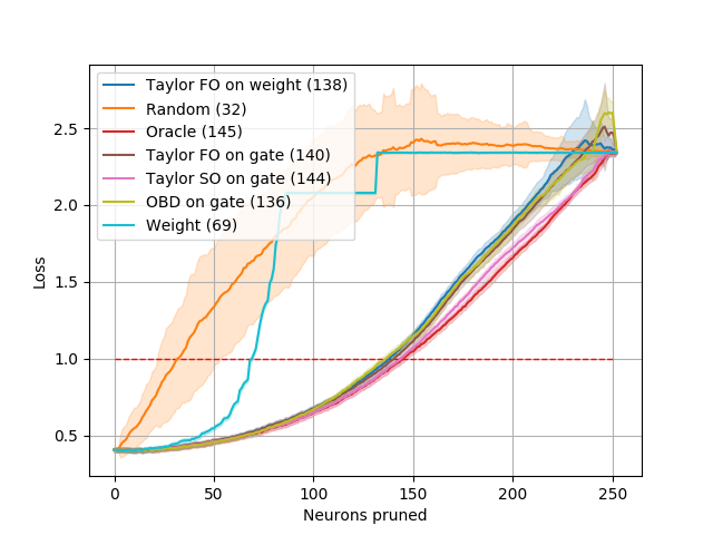 Figure 5
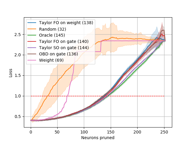 Figure 6
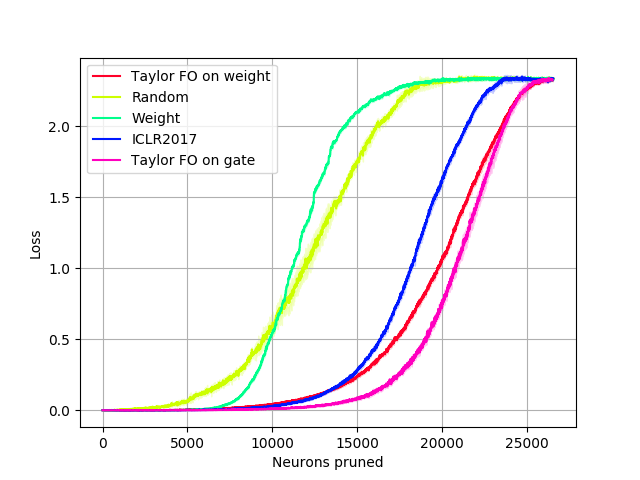 Figure 7
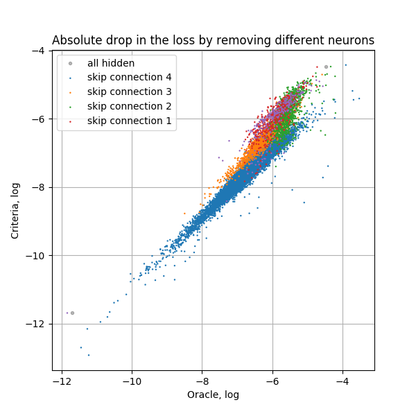 Figure 8
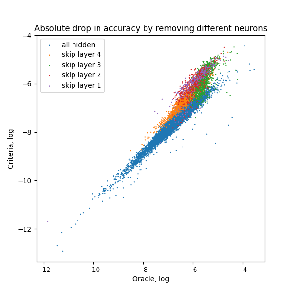 Figure 9
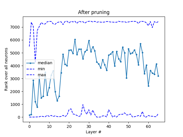 Figure 10
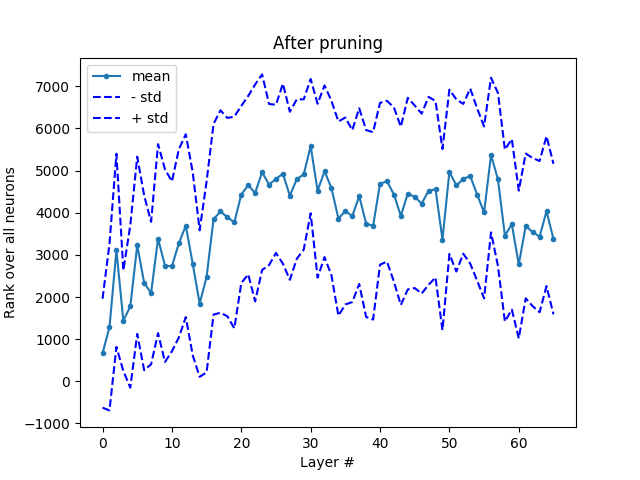 Figure 11
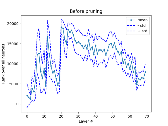 Figure 12
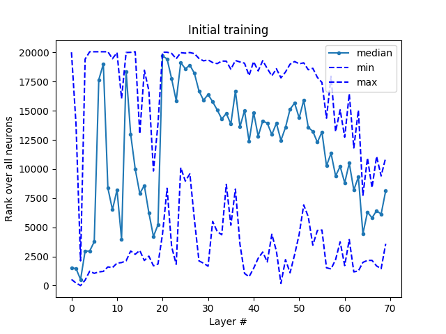 Figure 13
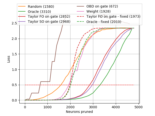 Figure 14
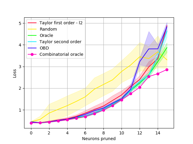 Figure 15
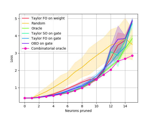 Figure 16
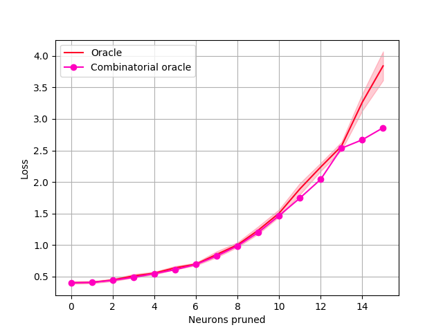 Figure 17
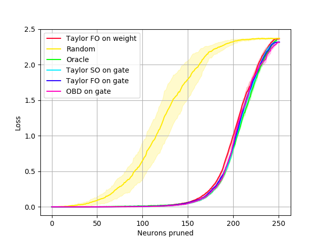 Figure 18
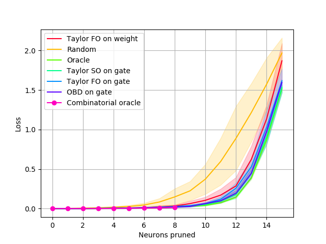 Figure 19
 Figure 20
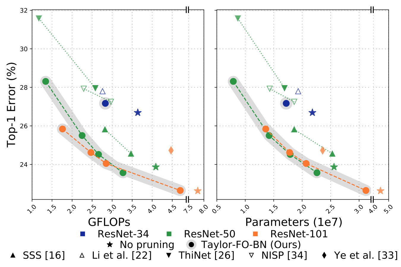 Figure 21
 Figure 22
 Figure 23
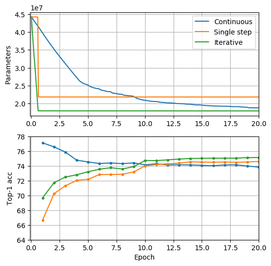 Figure 24
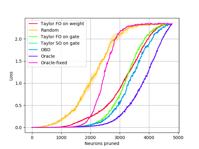 Figure 25
| Method | Residual block | All layers | |
|---|---|---|---|
| conv1 | conv2 | ||
| Taylor FO on conv weight | |||
| Weight magnitude | |||
| Gate after BN2 | |||
| Taylor FO | |||
| Taylor SO | |||
| OBD | |||
| Taylor FO - FG | |||
| Gate before BN2 | |||
| Taylor FO | |||
| Taylor SO | |||
| OBD | |||
| Taylor FO - FG | |||
| Method | Ours | Averaged per layer | All layers | ||||
|---|---|---|---|---|---|---|---|
| Taylor FO | Pearson | Spearman | Kendall | Pearson | Spearman | Kendall | |
| ResNet-101 | |||||||
| Gate after BN | ✓ | ||||||
| Gate after BN - FG | ✓ | ||||||
| Conv weight | ✓ | ||||||
| BN scale | ✓ | ||||||
| BN scale | |||||||
| Weight magnitude | |||||||
| Taylor-output [27] | |||||||
| Including skip connections | |||||||
| Gate after BN | ✓ | ||||||
| Gate after BN - FG | ✓ | ||||||
| VGG11-BN | |||||||
| Gate after BN | ✓ | ||||||
| Conv/Linear weight | ✓ | ||||||
| Gate after BN - FG | ✓ | ||||||
| BN scale | ✓ | ||||||
| BN scale | |||||||
| Weight magnitude | |||||||
| Taylor-output [27] | |||||||
| DenseNet-201 | |||||||
| Gate after BN | ✓ | ||||||
| Gate after BN - FG | ✓ | ||||||
| Conv weight | ✓ | ||||||
| BN scale | ✓ | ||||||
| BN scale | |||||||
| Weight magnitude | |||||||
| Taylor-output [27] | |||||||
| Pruning Method | GFLOPs | Params() | Error, |
| ResNet-101 | |||
| Taylor-FO-BN-40% (Ours) | |||
| Taylor-FO-BN-50% (Ours) | |||
| BN-ISTA v2 [33] | |||
| Taylor-FO-BN-55% (Ours) | |||
| BN-ISTA v1 [33] | |||
| No pruning | |||
| Taylor-FO-BN-75% (Ours) | |||
| pruning only skip connections | |||
| Taylor-FO-BN-52% (Ours) | |||
| Taylor-FO-BN-22% (Ours) | |||
| ResNet-50 | |||
| Taylor-FO-BN-56% (Ours) | |||
| Taylor-FO-BN-56% (No skip) | |||
| ThiNet-30 [26] | |||
| Taylor-FO-BN-72% (Ours) | |||
| NISP-50-B [34] | |||
| ThiNet-70 [26] | |||
| Taylor-FO-BN-81% (Ours) | |||
| SSS [16], ResNet-32 | |||
| NISP-50-A [34] | |||
| Taylor-FO-BN-91% (Ours) | |||
| No pruning | |||
| SSS [16], ResNet-41 | |||
| ResNet-34 | |||
| No pruning | |||
| Taylor-FO-BN-82% (Ours) | |||
| Li et al. [22] | |||
| VGG11-BN | |||
| No pruning | |||
| Taylor-FO-BN-50% (Ours) | |||
| From scratch [24] | |||
| Slimming [23], from [24] | |||
| DenseNet-201 | |||
| No pruning | |||
| Taylor-FO-BN-60% (Ours) | |||
| Taylor-FO-BN-36% (Ours) | |||
| No pruning | |||
| Strategy | Neurons | BN-ISTA [33] | Random | Oracle | Weight magnitude | OBD [21] | Taylor FO (Ours) | Taylor SO (Ours) |
|---|---|---|---|---|---|---|---|---|
| Prune A | 223() | 90.9% | 88.22(0.51) | 91.61(0.10) | 86.93(0.25) | 91.57 (0.15) | 91.52 (0.11) | 91.56 (0.14) |
| Prune A - train from scratch | 223() | 86.28(3.59) | 89.55(0.22) | 80.97(4.07) | 89.62(0.24) | 89.56(0.19) | 89.63(0.20) | |
| Prune B | 119() | 88.8% | 71.49(2.35) | 89.72(0.10) | 62.03(1.36) | 89.78 (0.16) | 89.78 (0.18) | 89.76 (0.17) |
| Prune B - train from scratch | 119() | 77.90(7.01) | 88.25(0.28) | 62.08(1.08) | 88.14(0.22) | 88.17(0.22) | 88.29(0.19) |
| Pruning Method | GFLOPs | Params() | Error, | Time, B16 | Time, B256 |
| No pruning | 7.80 | 4.47 | 22.63 | 29.0 | 379.8 |
| Taylor-FO-BN-75% | 4.70 | 3.12 | 22.65 | 24.1 | 313.5 |
| Taylor-FO-BN-55% | 2.85 | 2.07 | 24.05 | 21.6 | 261.7 |
| Taylor-FO-BN-50% | 2.47 | 1.78 | 24.62 | 20.9 | 251.4 |
| Taylor-FO-BN-40% | 1.76 | 1.36 | 25.84 | 21.0 | 223.4 |
| pruning only skip connections | |||||
| Taylor-FO-BN-52% | 6.57 | 3.60 | 22.94 | 25.3 | 326.7 |
| Taylor-FO-BN-22% | 5.19 | 2.86 | 24.77 | 19.5 | 239.3 |
Peer Reviews
No public reviews on file for this paper yet. If you reviewed it on a platform where reviews are public (OpenReview, ICLR, NeurIPS, ICML), you can paste yours below so the community can read it here.
Code & Models
Videos
No videos yet. Explain this paper in a talk, walkthrough, or lecture? Add one.
Taxonomy
MethodsPruning
Importance Estimation for Neural Network Pruning
Pavlo Molchanov, Arun Mallya, Stephen Tyree, Iuri Frosio, Jan Kautz
NVIDIA
{pmolchanov, amallya, styree, ifrosio, jkautz}@nvidia.com
Abstract
Structural pruning of neural network parameters reduces computation, energy, and memory transfer costs during inference. We propose a novel method that estimates the contribution of a neuron (filter) to the final loss and iteratively removes those with smaller scores. We describe two variations of our method using the first and second-order Taylor expansions to approximate a filter’s contribution. Both methods scale consistently across any network layer without requiring per-layer sensitivity analysis and can be applied to any kind of layer, including skip connections. For modern networks trained on ImageNet, we measured experimentally a high () correlation between the contribution computed by our methods and a reliable estimate of the true importance. Pruning with the proposed methods leads to an improvement over state-of-the-art in terms of accuracy, FLOPs, and parameter reduction. On ResNet-101, we achieve a 40% FLOPS reduction by removing 30% of the parameters, with a loss of 0.02% in the top-1 accuracy on ImageNet. Code is available at https://github.com/NVlabs/Taylor_pruning.
1 Introduction
Convolutional neural networks (CNNs) are widely used in today’s computer vision applications. Scaling up the size of datasets as well as the models trained on them has been responsible for the successes of deep learning. The dramatic increase in number of layers, from 8 in AlexNet [19], to over 100 in ResNet-152 [10], has enabled deep networks to achieve better-than-human performance on the ImageNet [31] classification task. Empirically, while larger networks have exhibited better performance, possibly due to the lottery ticket hypothesis [4], they have also been known to be heavily over-parameterized [35].
The growing size of CNNs may be incompatible with their deployment on mobile or embedded devices, with limited computational resources. Even in the case of cloud services, prediction latency and energy consumption are important considerations. All of these use cases will benefit greatly from the availability of more compact networks. Pruning is a common method to derive a compact network – after training, some structural portion of the parameters is removed, along with its associated computations.
A variety of pruning methods have been proposed, based on greedy algorithms [26, 34], sparse regularization [20, 22, 33], and reinforcement learning [12]. Many of them rely on the belief that the magnitude of a weight and its importance are strongly correlated. We question this belief and observe a significant gap in correlation between weight-based pruning decisions and empirically optimal one-step decisions – a gap which our greedy criterion aims to fill.
We focus our attention on extending previously proposed methods [1, 21, 27] with a new pruning criterion and a method that iteratively removes the least important set of neurons (typically filters) from the trained model. We define the importance as the squared change in loss induced by removing a specific filter from the network. Since computing the exact importance is extremely expensive for large networks, we approximate it with a Taylor expansion (akin to [27]), resulting in a criterion computed from parameter gradients readily available during standard training. Our method is easy to implement in existing frameworks with minimal overhead.
Additional benefits of our novel criterion include: a) no hyperparameters to set, other than providing the desired number of neurons to prune; b) globally consistent scale of our criterion across network layers without the need for per-layer sensitivity analysis; c) a simple way of computing the criterion in parallel for all neurons without greedy layer-by-layer computation; and d) the ability to apply the method to any layer in the network, including skip connections. We highlight our main contributions below:
- •
We propose a new method for estimating, with a little computational overhead over training, the contribution of a neuron (filter) to the final loss. To do so, we use averaged gradients and weight values that are readily available during training.
- •
We compare two variants of our method using the first and second-order Taylor expansions, respectively, against a greedy search (“oracle”), and show that both variants achieve state-of-the-art results, with our first-order criteria being significantly faster to compute with slightly worse accuracy.
We also find that using a squared loss as a measure for contribution leads to better correlations with the oracle and better accuracy when compared to signed difference [21].
Estimated Spearman correlation with the oracle on ResNets and DenseNets trained on ImageNet show significant agreement (>), a large improvement over previous methods [16, 21, 22, 27, 33], leading to improved pruning.
- •
Pruning results on a wide variety of networks trained on CIFAR-10 and ImageNet, including those with skip connections, show improvement over state-of-the-art.
2 Related work
One of the ways to reduce the computational complexity of a neural network is to train a smaller model that can mimic the output of the larger model. Such an approach, termed network distillation, was proposed by Hinton et al. [14].
The biggest drawback of this approach is the need to define the architecture of the smaller distilled model beforehand.
Pruning – which removes entire filters, or neurons, that make little or no contribution to the output of a trained network – is another way to make a network smaller and faster. There are two forms in which structural pruning is commonly applied: a) with a predefined per-layer pruning ratio, or b) simultaneously over all layers. The second form allows pruning to automatically find a better architecture, as demonstrated in [24]. An exact solution for pruning will be to minimize the norm of all neurons and remove those that are zeroed-out. However, minimization is impractical as it is non-convex, NP-hard, and requires combinatorial search. Therefore, prior work has tried to relax the optimization using Bayesian methods [25, 29] or regularization terms.
One of the first works that used regularization, by Hanson and Pratt [8], used weight decay along with other energy minimization functions to reduce the complexity of the neural network. At the same time, Chauvin [1] discovered that augmenting the loss with a positive monotonic function of the energy term can lead to learning a sparse solution.
Motivated by the success of sparse coding, several methods relax minimization with or regularization, followed by soft thresholding of parameters with a predefined threshold. These methods belong to the family of Iterative Shrinkage and Thresholding Algorithms (ISTA) [3]. Han et al. [7] applied a similar approach for removing individual weights of a neural network to obtain sparse non-regular convolutional kernels. Li et al. [22] extended this approach to remove filters with small norms.
Due to the popularity of batch-normalization [17] layers in recent networks [10, 15], several approaches have been proposed for filter pruning based on batch-norm parameters [23, 33]. These works regularize the scaling term () of batch-norm layers and apply soft thresholding when value fell below a predefined threshold. Further, FLOPS-based penalties can also be included to directly reduce computational costs [5]. A more general scheme that uses an ISTA-like method on scaling factors was proposed by [16] and can be applied to any layer.
All of the above methods explicitly rely on the belief that the magnitude of the weight or neuron is strongly correlated with its importance. This belief was investigated as early as 1988 by Mozer [28] who proposed adding a gating function after each layer to be pruned. With gate values initialized to , the expectation of the negative gradient is used as an approximation for importance. Mozer noted that weights magnitude merely reflect the statistics of importance. LeCun et al. [21] also questioned whether magnitude is a reasonable measure of neuron importance. The authors suggested using a product of the Hessian’s diagonal and the squared weight as a measure of individual parameter importance, and demonstrated improvement over magnitude-only pruning.
This approach assumes that after convergence, the Hessian is a positive definite matrix, meaning that removing any neuron will only increase the loss. However, due to stochasticity in training with minibatches under a limited observation set and in the presence of saddle points, there do exist neurons whose removal will decrease the loss.
Our method does not assume that the contribution of all neurons is strictly positive. Therefore, we approximate the squared difference of the loss when a neuron is removed and can do so with a first-order or second-order approximation, if the Hessian is available.
A few works have estimated neuron importance empirically. Luo et al. [26] propose to use a greedy per-layer procedure to find the subset of neurons that minimize a reconstruction loss, at a significant computational cost. Yu et al. [34] estimate the importance of input features to a linear classifier and propagate their importance assuming Lipschitz continuity, requiring additional computational costs and non-trivial implementation of the feature score computation. Our proposed method is able to outperform these methods while requiring little additional computation and engineering.
Pruning methods such as [12, 13, 22, 26, 34] require sensitivity analysis in order to estimate the pruning ratio that should be applied to particular layers. Molchanov et al. [27] assumed all layers have the same importance in feed-forward networks and proposed a normalization heuristic for global scaling. However, this method fails in networks with skip connections. Further, it computes the criterion using network activations, which increases memory requirements. Conversely, pruning methods operating on batch-normalization [5, 16, 23, 33] do not require sensitivity analysis and can be applied globally. Our criterion has globally-comparable scaling by design and does not require sensitivity analysis. It can be efficiently applied to any layer in the network, including skip connections, and not only to batch-norm layers.
A few prior works have utilized pruning as a network training regularizer. Han et al. [6] re-initialize weights after pruning and finetune them to achieve even better accuracy than the initial model. He et al. [11] extend this idea by training filters even after they were zeroed-out. While our work focuses only on removing filters from networks, it might be possible to extend it as a regularizer.
3 Method
Given neural network parameters and a dataset composed of input () and output () pairs, the task of training is to minimize error by solving:
[TABLE]
In the case of pruning we can include a sparsification term in the cost function to minimize the size of the model:
[TABLE]
where is a scaling coefficient and is the norm which represents the number of non-zero elements. Unfortunately there is no efficient way to minimize the norm as it is non-convex, NP-hard, and requires combinatorial search.
An alternative approach starts with the full set of parameters upon convergence of the original optimization (1) and gradually reduces this set by a few parameters at a time. In this incremental setting, the decision of which parameters to remove can be made by considering the importance of each parameter individually, assuming independence of parameters. We refer to this simplified approximation to full combinatorial search as greedy first-order search.
The importance of a parameter can be quantified by the error induced by removing it. Under an i.i.d. assumption, this induced error can be measured as a squared difference of prediction errors with and without the parameter ():
[TABLE]
Computing for each parameter, as in (3), is computationally expensive since it requires evaluating versions of the network, one for each removed parameter.
We can avoid evaluating different networks by approximating in the vicinity of W by its second-order Taylor expansion:
[TABLE]
where are elements of the gradient g, are elements of the Hessian H, and is its m-th row. An even more compact approximation is computed using the first-order expansion, which simplifies to:
[TABLE]
The importance in Eq. (5) is easily computed since the gradient g is already available from backpropagation. For the rest of this section we will primarily use the first-order approximation, however most statements also hold for the second-order approximation. Future reference we denote the set of first-order importance approximations:
[TABLE]
To approximate the joint importance of a structural set of parameters , e.g. a convolutional filter, we have two alternatives. We can define it as a group contribution:
[TABLE]
or, alternatively, sum the importance of the individual parameters in the set,
[TABLE]
For insight into these two options, and to simplify calculations, we add “gates” to the network, , with weights equal to and dimensionality equal to the number of neurons (feature maps) . Gating layers make importance score computation easier, as they: a) are not involved in optimization; b) have a constant value, therefore allowing W to be omitted from Eq. (4-8); and c) implicitly combine the contributions of filter weights and bias.
If a gate follows a neuron parameterized by weights , then the importance approximation is:
[TABLE]
where represents the inner dimensions needed to compute the output of the previous layer, e.g. input dimension for a linear layer, or spatial and input dimensions for a convolutional layer. We see that gate importance is equivalent to group contribution on the parameters of the preceding layer.
Through some manipulation, we can make a connection to information theory from our proposed method. Let’s denote and observe (under the assumption that, at convergence, ):
[TABLE]
where the variance is computed across observations.
If the error function is chosen to be the log-likelihood function, then assuming the gradient is estimated as , borrowing from concepts in information theory [2], we obtain
[TABLE]
where is the expected Fisher information matrix. We conclude that the variance of the gradient is the expectation of the outer product of gradients and is equal to the expected Fisher information matrix. Therefore, the proposed metric, , can be interpreted as the variance estimate and as the diagonal of the Fisher information matrix. Similar conclusion was drawn in [32].
3.1 Pruning algorithm
Our pruning method takes a trained network as input and prunes it during an iterative fine-tuning process with a small learning rate. During each epoch, the following steps are repeated:
For each minibatch, we compute parameter gradients and update network weights by gradient descent. We also compute the importance of each neuron (or filter) using the gradient averaged over the minibatch, as described in (7) or (8). (Or, the second-order importance estimate may be computed if the Hessian is available.) 2. 2.
After a predefined number of minibatches, we average the importance score of each neuron (or filter) over the of minibatches, and remove the neurons with the smallest importance scores.
Fine-tuning and pruning continue until the target number of neurons is pruned, or the maximum tolerable loss can no longer be achieved.
3.2 Implementation details
Hessian computation. Computing the full Hessian in Eq. (4) is computationally demanding, thus we use a diagonal approximation. During experiments with ImageNet we cannot compute the Hessian because of memory constraints.
Importance score accumulation. During training or fine-tuning with minibatches, observed gradients are combined to compute a single importance score \hat{\textbf{I}}={\mathbb{E}}\big{\langle}\textbf{I}\big{\rangle}.
Importance score aggregation. In this work, we compute the importance of structured parameters as a sum of individual contributions defined in Eq. (8), unless gates are used automatically compute the group contribution on the parameters from the preceding layer. Second-order methods are always computed on gates. We observed that the “group contribution” criterion in Eq. (7) exhibits very low correlation with the “true” importance (3) if the parameter set is too large, due to expectation of gradients tending to zero at convergence.
Gate placement. Unless otherwise stated, gates are placed immediately after a batch normalization layer to capture contributions from scaling and shifting parameters simultaneously. The first-order criterion computed for a feature map at the gate can be shown to be with and being the scale and shift parameters of the batch normalization.
Averaging importance scores over pruning iterations. We average importance scores between pruning iterations using an exponential moving average filter (momentum) with coefficient .
Pruning strategy. We found that the method performs better when we define the number of neurons to be removed, prune them in batches and fine-tune the network after that. An alternative approach is to continuously prune as long as the training or validation loss is below the threshold. The latter approach leads the optimization into local minima and final results are slightly worse.
Number of minibatches between pruning iterations needs be sufficient to capture statistics of the overall data. We use minibatches and a small batch size for CIFAR datasets, but a larger () batch size and minibatches for ImageNet pruning, as noted with each experiment.
Number of neurons pruned per iteration needs to be chosen based on how correlated the neurons are to each other. We observed that a filter’s contribution changes during pruning and we usually prune around of initial filters per iteration.
4 Experiments
We evaluate our method on a variety of neural network architectures on the CIFAR-10 [18] and ImageNet [31] datasets. We also experiment with variations of our method to understand the best variant. Whenever we refer to Weight, Weight magnitude or BN scale, we use norm.
4.1 Results on CIFAR-10
With the CIFAR-10 dataset, we evaluate “oracle” methods and second-order methods by pruning smaller networks, including LeNet3 and variants of ResNets [9] and pre-activation ResNets [10].
4.1.1 LeNet3
We start with a simple network, LeNet3, trained on the CIFAR-10 dataset to achieve test accuracy. The architecture of LeNet consists of convolutional and linear layers arranged in a C-R-P-C-R-P-L-R-L-R-L (C: Conv, R: ReLU, P: Pooling, L: Linear) order with , , , , and neurons respectively. We prune the first convolutional and first linear layers without changing the output linear layer or finetuning after pruning.
Single layer pruning. In this setup, we only prune the first convolutional layer. This setting allows us to use the Combinatorial oracle, the true minimizer: we compute the loss for all possible combinations of neurons that can be pruned and pick the best one. Note that this requires an exponential number of feedforward passes to evaluate – per , where is the number of filters and is number of filters to prune, and so is not practical for multiple layers or larger networks. We compare against a greedy search approximation, the Greedy oracle, that exhaustively finds the single best neuron to remove at each pruning step, repeated times. Results shown in Fig. 2 show the loss vs. the number of neurons pruned. We observe that the Combinatorial oracle is not significantly better than the Greedy oracle when pruning a small number of neurons. Considering that the former has exponential computational complexity, in subsequent experiments we use the Greedy oracle (referred to simply as Oracle) as a representation of the best possible outcome.
All layers pruning.
Fig. 3 shows pruning results when all layers are pruned using various criteria. We refer to our methods based on the Taylor expansion as Taylor FO/Taylor SO, indicating the order of the approximation used, first- and second-order, respectively. We consider both a direct application to convolutional filter weights (“on weight”) and the use of gates following each convolutional layer (“on gate”).] We treat linear layers as convolutions. In all cases, pruning removes the entire filter and its corresponding bias. At each pruning iteration, we remove the neuron with the least importance as measured by the criterion used, and measure the loss on the training set.
Results in Fig. 3 show that Oracle pruning performs best, followed closely by the second- and first-order Taylor expansion criteria, respectively. Both first and second-order Taylor methods prune nearly the same number of neurons as the Oracle before exceeding the loss threshold. Weight-based pruning, which removes neurons with the least norm, performs as poorly as randomly removing neurons. OBD [21] performs similarly to the Oracle and Taylor methods.
The experiments on LeNet confirm the following: (1) The greedy oracle closely follows the pruning performance of the Combinatorial oracle for small changes to the network, while being exponentially faster to compute. (2) Our first-order method (Taylor FO) is comparable to the second-order method (Taylor SO) in this setting.
4.1.2 ResNet-18
Now we compare pruning criteria on the more complex architecture ResNet-18, from the pre-activation family [10]. Each residual block has an architecture of BN1-ReLU-conv1-BN2-ReLU-conv2, together with a skip connection from the input to the output, repeated for a total of blocks. Trained on CIFAR-10, ResNet-18 achieves a test accuracy of . For pruning, we consider entire feature maps in the conv layers as they command the largest share of computational resources.
In these experiments, we examine the following ways of estimating our criterion: (1) Applying it directly on convolutional filter weights, (2) Using gates placed before BN2 and after conv2, and (3) Using gates placed after BN2 and after conv2. We remove neurons every minibatches, and report final results averaged over seeds. We also compare using gradients averaged over a mini-batch and gradients obtained per data sample, the latter denoted by “full grad”, or “FG”. We should note that using the full gradient changes the gate formulation from computing the group contribution (Eq. 7) to the sum of individual contributions (Eq. 8).
Table 1 presents the Spearman correlation between various pruning criteria and the greedy oracle. Results in the Residual block column are averaged over all blocks. The All layers column includes additional layers: the first convolutional layer (not part of residual blocks), all convolutions in residual blocks, and all strided convolutions. We observe that placing the gate before BN2 significantly reduces correlation – correlation for conv1 drops from to for Taylor FO, suggesting that the subsequent batch-normalization layer significantly affects criteria computed from the gate. We observe that the effect is less significant when the full gradient is used, however it shows smaller correlation overall with the oracle. OBD has lower correlation than our Taylor based methods. The highest correlation is observed for Taylor SO, with Taylor FO following right after. As placing gates after BN2 dramatically improves the results, this indicates that the batch-normalization layers play a key role in determining the contribution of the corresponding filter.
Results of pruning ResNet-18 without fine-tuning are shown in Fig. 4. We observe that the oracle achieves the best accuracy for a given number of pruned neurons. All methods, except “-fixed” and Random, recompute the criteria after each iterative step and can adjust to the pruned network. Oracle-fixed and Taylor FO-fixed are computed across the same number of batches as non-fixed criteria. We notice that fixed criteria clearly perform significantly worse than oracle, emphasizing importance of reestimating the criteria after each pruning iteration, allowing the values to adjust to changes in the network architecture.
An interesting observation is that the OBD method performs poorly in spite of having a good correlation with the oracle in Table 1. The reason for this discrepancy is that when we evaluate correlation with the oracle, we square estimates of OBD to make them comparable to the way the oracle was estimated. However, during pruning, we use signed values of OBD, as was prescribed in [21]. As mentioned earlier, for deep networks, the diagonal of the Hessian is not positive for all elements and removing those with negative impact results in increased network instability. Therefore, without fine-tuning, OBD is not well suited for pruning. Another important observation is that if the Hessian is available, using the Taylor SO expansion can get both better pruning and correlation. Surprisingly, we observe no improvement in using the full gradient, probably because of the switch in contributions from group to individual.
At this stage, after experiments with the small LeNet3 network the larger ResNet-18 on the CIFAR-10 dataset, we make the following observations: (1) Our proposed criteria based on the Taylor expansion of the pruning loss have a very high correlation with the neuron ranking produced by the oracle. (2) The first- and second-order Taylor criteria are comparable. As the Taylor FO can be computed much faster with a lower memory footprint, further experiments with larger networks on ImageNet are performed using this criterion only.
4.2 Results on ImageNet
Here, we apply our method on the challenging task of pruning networks trained on ImageNet [31], specifically the ILSVRC2012 version. For all experiments in this section, we use PyTorch [30] and default pretrained models as a starting point for network pruning. We use standard preprocessing and augmentation: re-sizing images to have a smallest dimension of , randomly cropping a patch, randomly applying horizontal flips, and normalizing images by subtracting a per-dataset mean and dividing by a per-dataset standard deviation. During testing, we use the central crop of size .
4.2.1 Neuron importance correlation study
We compare against pruning methods that use various heuristics, such as weight magnitude [20, 22], magnitude of the batch-norm scale, BN scale [5, 23, 33], and output-based heuristics (Taylor expansion applied to layer outputs) [27].
We estimate the correlation between the “real importance” of a filter and these criteria. Estimating real importance, or the change in loss value upon removing a neuron, requires running inference multiple times while setting each individual filter to [math] in turn. (Note that the oracle ranks neurons based on this value). For ResNet-101, we pruned filters in the first convolutional layers of every residual block. Separately, we add gates to skip connections at the input and output of each block. For the VGG11-BN architecture, we replace drop-out layers with batch-norms ( scale and [math] shift) and fine-tune for epochs until test accuracy reaches to be comparable with [24]. For DenseNet201, we considered features after the batch-norm layer that follows the first convolution in every dense layer.
The statistical correlation between heuristics and measured importance are summarized in Table 2. Correlations were measured on a subset of ImageNet consisting of a few thousand images. We evaluated various implementations of our method, but always use the first-order Taylor expansion, denoted Taylor FO. As previously discussed, the most promising variation uses a gate after each batch-norm layer. The All layers correlation columns show how well the criteria scale across layers. Our method exhibits > Spearman correlation for all three networks. Weight magnitude and BN scale have quite low correlation, suggesting that magnitude is not a good representation of importance. Output-based expansion proposed in [27] has high correlation on the VGG11-BN network but fails on ResNet and DenseNet architectures. Surprisingly, we observe > Pearson correlation for ResNet and DenseNet, showing we can almost exactly predict the change in loss for every neuron.
We are also able to study the effect of skip connections by adding a gate after the output of each residual block. We add skip connections to the full set of filters and evaluate their correlation, denoted “Including skip connections” in Table 2. We observe high correlation of the criterion with skip connections as well. Given this result, we adopt this methodology for pruning ResNets and remove channels from skip connections and bottleneck layers simultaneously. We refer to this variant of our method as Taylor-FO-BN.
4.2.2 Pruning and fine-tuning
We use the following settings: GPUs and a batch size of examples; we optimized using SGD with initial learning rate (or , see Sec. 6.2) decayed a factor every epochs, momentum set to ; pruning and fine-tuning run for epochs total; we report the best validation accuracy observed. Every mini-batches we remove neurons until we reach the predefined number of neurons to be pruned, after which we reset the momentum buffer and continue fine-tuning. By setting the percentage of neurons to remain after pruning to be X, we get different versions of the final model and refer to them as Taylor-FO-BN-X%.
Comparison of pruning networks on ImageNet by the proposed method and other methods is presented in the Table 3, where we report total number of FLOPs, number of parameters, and the top-1 error rate. Comparison is grouped by network architecture type and the number of parameters. For ResNet-101 we observe smaller error rates and fewer GFLOPs (by at least GFLOPs) when compare to BN-ISTA method [33]. Pruning only skip connections shows larger errors however makes the final network faster (see Sec 6.2). By pruning of FLOPs and of parameters from original ResNet-101 we only lose in accuracy. Pruning results on ResNet-50 and ResNet-34 demonstrate significant improvements over other methods. Additionally we study our method without pruning skip connections, marked as “No skip” and observe accuracy loss. Comparison per layer ranking of different layers in ResNet-101 before and after pruning is shown in Fig. 5.
Pruning neurons with a single step. As an alternative to iterative pruning, we performed pruning of neurons with a single step after mini-batches, followed by fine-tuning. This gave a top-1 error of , which is % higher than Taylor-FO-BN-50%, again emphasizing the benefit of re-evaluating the criterion between pruning iterations.
Pruning other networks. We also prune the VGG11-BN and DenseNet networks. The former is a simple feed-forward architecture, without skip connections. We prune of neurons across all layers, as per prior work [24, 23]. Our approach shows only loss in accuracy after removing of parameters and improves on the previously reported results by [24] and more than [23]. DeseNets reuse feature maps multiple times, potentially making them less amenable to pruning. We prune DenseNet-201 and observe that with the same number of FLOPs (Taylor-FO-BN-52%) as DenseNet-121, we have lower error.
5 Conclusions
In this work, we have proposed a new method for estimating the contribution of a neuron using the Taylor expansion applied on a squared change in loss induced by removing a chosen neuron. We demonstrated that even the first-order approximation shows significant agreement with true importance, and outperforms prior work on a range of deep networks. After extensive analysis, we showed that applying the first-order criterion after batch-norms yields the best results, under practical computational and memory constraints.
6 Supplementary material
In supplementary material we show additional experimental results on ResNet20 with CIFAR10, ResNet101 on ImageNet. Additionally, we evaluate inference speed of pruned ResNet101 models.
6.1 ResNet20 on CIFAR10
We experiment on ResNet20 trained on CIFAR10 in order to compare with the work of [33] (referred to as BN-ISTA) and to evaluate the effect of the “pruning paradox” reported in [24]. Our setup is as follows: initial model was trained for epochs with learning rate and decay by after epochs. Final model obtained on the test split and we picked it as an initial model for pruning. Pruning and fine-tuning setup is: initial learning rate of , decayed by every epochs for a total number of epochs. While pruning, we remove neurons every mini-batches until the predefined number of pruned neurons is reached.
Results of pruning and training from scratch are summarized in the Table 4. We observe that pruning with Random or magnitude based criteria results in the worst performance, primary because they introduce uncorrelated bias to the estimate, we also observe that these 2 methods can be affected by ”pruning paradox” as their difference is within a standard deviation of experiments. Our proposed method that relies on estimating feature importance with Taylor expansion of first and second orders outperform BT-ISTA[33]. The difference between Optimal Brain Damage and Our methods is not large and within a single standard deviation. We conclude that first order Taylor expansion applied to the gates after BN is a reasonable choice for residual network. It is not affected by ”prunung paradox” discovered in [24].
6.2 Additional details on ResNets pruning
Our method can be applied with various pruning scheduling. The scheduling we apply in the paper, named here as iterative, removes 100 neurons per every 30 mini-batch updates until we reach predefined number of neurons. Also, all neurons can be removed at once, named as pruning with a single step. One more setting, named as continuous, prunes 100 neurons every 30 mini-batches only if the training loss is above the predefined threshold (we set it to 1.04).
Progress of ResNet-101 pruning on ImageNet with 3 different pruning scheduling settings is illustrated in Fig. 6. All settings had the maximum number of neurons to be pruned as 10000 out of 20096, and the Iterative corresponds to TaylorFO-BN-50% in the main paper. Iterative pruning clearly outperforms other settings over all epochs.
Finetuning details on ImageNet dataset.
When a large number of neurons are removed we found that starting with the larger learning rate works better. Therefore we use starting learning of for the following pruning models: ResNet-101 ( Taylor-FO-BN-40% and Taylor-FO-BN-22%), ResNet-50 (Taylor-FO-BN-56%). All other networks were finetuned with initial learning of . Weight decay is set to during finetuning.
Inference speed.
The main reason behind filter level pruning is computation cost reduction. We evaluate inference time of pruned models in the Table 5. Pruning results in inference speed reduction, especially for the larger batch size. Pruning skip connections results in higher time reduction compared to pruning all layers. For example, only by removing 33% of FLOPs result in 1.59 speed up of Taylor-FO-BN-22%, while by removing 68% of FLOPs results only in 1.51 speed up of Taylor-FO-BN-50%.
6.3 Oracle computation details
Oracle for Table 2 is computed from the training set (as [27]) with Eq. (3). To check if correlation study is representative we compute the Oracle from the test set. Correlation between Oracles computed on training and testing sets, respectively, is . After recomputing Table 2 using the test set, we observed little change (avg. deviation of between raw table entries) and no reordering of the methods.
The reference list from the paper itself. Each links out to its DOI / PubMed record.
- 1[1] Y. Chauvin. A back-propagation algorithm with optimal use of hidden units. In NIPS , 1989.
- 2[2] T. M. Cover and J. A. Thomas. Elements of information theory . John Wiley & Sons, 2012.
- 3[3] I. Daubechies, M. Defrise, and C. De Mol. An iterative thresholding algorithm for linear inverse problems with a sparsity constraint. Communications on Pure and Applied Mathematics , 2004.
- 4[4] J. Frankle and M. Carbin. The lottery ticket hypothesis: Training pruned neural networks. ar Xiv preprint ar Xiv:1803.03635 , 2018.
- 5[5] A. Gordon, E. Eban, O. Nachum, B. Chen, H. Wu, T.-J. Yang, and E. Choi. Morphnet: Fast & simple resource-constrained structure learning of deep networks. In CVPR , 2018.
- 6[6] S. Han, J. Pool, S. Narang, H. Mao, S. Tang, E. Elsen, B. Catanzaro, J. Tran, and W. J. Dally. Dsd: regularizing deep neural networks with dense-sparse-dense training flow. ar Xiv preprint ar Xiv:1607.04381 , 2016.
- 7[7] S. Han, J. Pool, J. Tran, and W. Dally. Learning both weights and connections for efficient neural network. In NIPS , 2015.
- 8[8] S. J. Hanson and L. Y. Pratt. Comparing biases for minimal network construction with back-propagation. In NIPS , 1989.
