Distributed Optimization for Smart Cyber-Physical Networks
Giuseppe Notarstefano, Ivano Notarnicola, Andrea Camisa

TL;DR
This paper surveys distributed optimization methods enabling smart cyber-physical network agents to cooperatively solve large-scale problems through local computation and communication without central coordination.
Contribution
It formalizes principal distributed optimization approaches and reviews recent extensions, providing a comprehensive introduction to the field.
Findings
Consensus-based, duality-based, and constraint exchange methods are key approaches.
Basic schemes are analyzed for effectiveness and efficiency.
State-of-the-art extensions improve scalability and robustness.
Abstract
The presence of embedded electronics and communication capabilities as well as sensing and control in smart devices has given rise to the novel concept of cyber-physical networks, in which agents aim at cooperatively solving complex tasks by local computation and communication. Numerous estimation, learning, decision and control tasks in smart networks involve the solution of large-scale, structured optimization problems in which network agents have only a partial knowledge of the whole problem. Distributed optimization aims at designing local computation and communication rules for the network processors allowing them to cooperatively solve the global optimization problem without relying on any central unit. The purpose of this survey is to provide an introduction to distributed optimization methodologies. Principal approaches, namely (primal) consensus-based, duality-based and…
Click any figure to enlarge with its caption.
 Figure 1
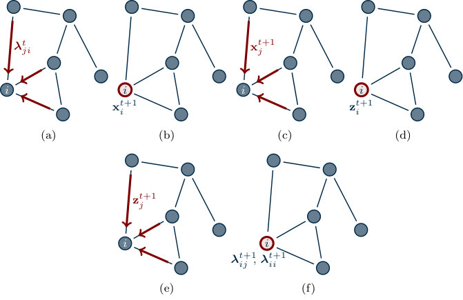 Figure 2
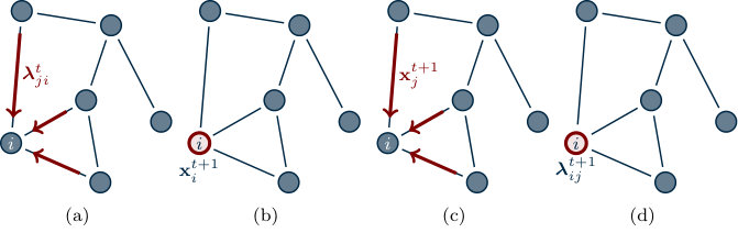 Figure 3
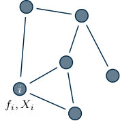 Figure 4
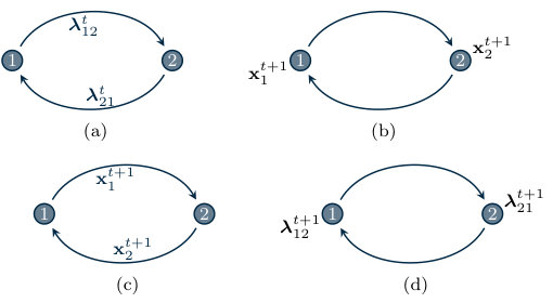 Figure 5
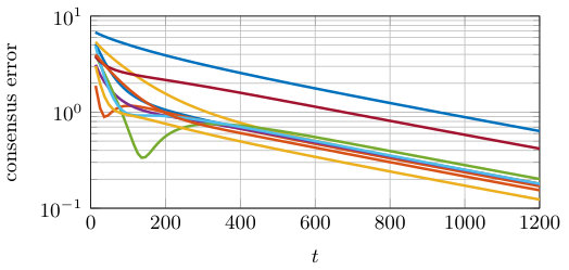 Figure 6
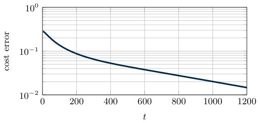 Figure 7
 Figure 8
 Figure 9
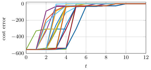 Figure 10
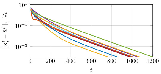 Figure 12
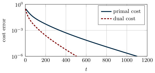 Figure 13
 Figure 15
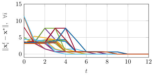 Figure 16
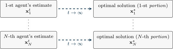 Figure 19
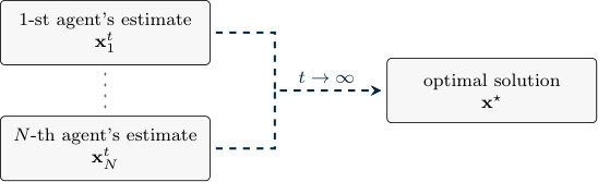 Figure 20
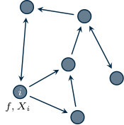 Figure 22
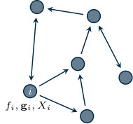 Figure 23
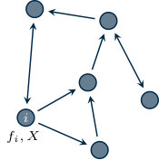 Figure 24
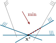 Figure 27
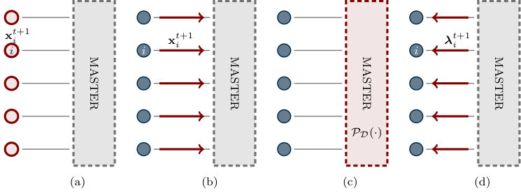 Figure 28
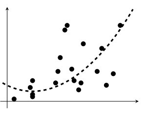 Figure 29
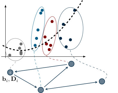 Figure 30
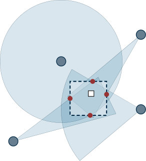 Figure 31
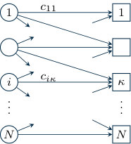 Figure 32
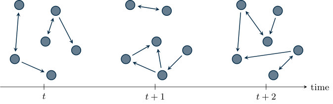 Figure 33
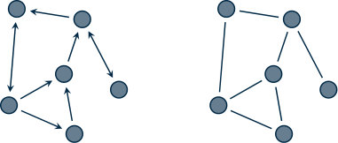 Figure 34
Peer Reviews
No public reviews on file for this paper yet. If you reviewed it on a platform where reviews are public (OpenReview, ICLR, NeurIPS, ICML), you can paste yours below so the community can read it here.
Videos
No videos yet. Explain this paper in a talk, walkthrough, or lecture? Add one.
Distributed Optimization for
Smart Cyber-Physical Networks
Notarstefano, Giuseppe
Università di Bologna, Bologna (Italy)
Notarnicola, Ivano
Università di Bologna, Bologna (Italy)
Camisa, Andrea
Università di Bologna, Bologna (Italy)
Abstract
The presence of embedded electronics and communication capabilities as well as sensing and control in smart devices has given rise to the novel concept of cyber-physical networks, in which agents aim at cooperatively solving complex tasks by local computation and communication. Numerous estimation, learning, decision and control tasks in smart networks involve the solution of large-scale, structured optimization problems in which network agents have only a partial knowledge of the whole problem. Distributed optimization aims at designing local computation and communication rules for the network processors allowing them to cooperatively solve the global optimization problem without relying on any central unit. The purpose of this survey is to provide an introduction to distributed optimization methodologies. Principal approaches, namely (primal) consensus-based, duality-based and constraint exchange methods, are formalized. An analysis of the basic schemes is supplied, and state-of-the-art extensions are reviewed.
Contents
-
3.2 Distributed Dual Decomposition for Cost-Coupled Problems
-
3.4 Distributed Dual Methods for Constraint-Coupled Problems
-
3.4.1 Connections between Cost-Coupled and Constraint-Coupled Problems via Duality
-
4.3.2 Distributed Mixed-Integer Linear Programming via Cut Generation and Constraint Exchange
Introduction
Motivation
In recent years, the breakthroughs in embedded electronics are giving the opportunity to include computation and communication capabilities in almost any device of several domains as factories, farms, buildings, grids and cities. Communication among devices has enabled a number of new challenges along the direction of turning smart devices into smart (cooperating) systems. The keyword “cyber-physical networks” is being adopted to refer to this permeating reality, whose distinctive feature is that a great advantage can be obtained if its interconnected, complex nature is exploited. A novel peer-to-peer distributed computational framework is emerging as a new opportunity in which peer processors, communicating over a network, cooperatively solve a task without resorting to a unique provider that knows and owns all the data.
Several challenges arising in cyber-physical networks can be stated as optimization problems. Examples are estimation, decision, learning and control applications. To solve optimization problems over cyber-physical networks, it is not possible to apply the classical optimization algorithms (that we call centralized), which require the data to be managed by a single entity. In fact, the problem data are spread over the network, and it is undesirable (or even impossible) to collect them at a unique node. To this end, parallel computing serves as a source of inspiration. In order to speed up the solution of large-scale optimization problems, several effort has been made in designing parallel algorithms by splitting the computational burden among several processors. However, for typical parallel optimization algorithms, a central coordinating node is required and the communication topology is designed ad hoc. In distributed computation the communication topology cannot be thought of as a design parameter. Rather, it is a given part of the problem. Thus, in cyber-physical networks, the goal is to design algorithms, based on the exchange of information among the processors, that take advantage of the aggregated computational power. All the agents must be treated as peers and each of them must perform the same tasks and no “master” node must be present. Moreover, information privacy is often a requirement (i.e., private problem data at each node must not be shared with the other nodes). These challenges call for tailored strategies and have given rise to a novel, growing research branch termed distributed optimization.
Scope of the Monograph
The purpose of this survey is to give a comprehensive overview of the most common approaches used to design distributed optimization algorithms, together with the theoretical analysis of the main schemes in their basic version. We identify and formalize classes of problem set-ups that arise in motivating application scenarios. For each set-up, in order to give the main tools for analysis, we review tailored distributed algorithms in simplified cases. Extensions and generalizations of the basic schemes are also discussed at the end of each chapter. The algorithms have been developed by combining mathematical tools from optimization theory (e.g., duality) and network control theory (e.g., average consensus). For some of the discussed algorithms, we will present also parallel algorithms that serve as a starting point for the development of distributed methods.
We focus on three main categories of distributed optimization approaches: (i) primal consensus-based methods, i.e., methods combining classical gradient or subgradient steps with local averaging schemes; (ii) dual methods, i.e., methods which employ the Lagrangian dual of suitable equivalent formulations of the target problem to obtain a distributed routine; (iii) constraint exchange methods, which are based on the exchange of (active) constraints among agents to compute a solution of the considered problem.
Survey papers on distributed optimization have been proposed in the literature. An early survey paper presenting a broad class of relevant optimization problems in control is [1]. It also discusses tailored, parallel and distributed optimization algorithms based on decomposition techniques and including also the distributed subgradient method. Recent surveys analyze thoroughly average consensus [2] and the distributed subgradient method [2, 3, 4], with a literature review on other distributed optimization techniques. The book [5] provides parallel and distributed asynchronous optimization algorithms, including gradient tracking techniques. Some latest advances in distributed optimization are collected in [6].
Organization
In Chapter 1, we introduce the relevant problem set-ups, that we call cost-coupled, constraint-coupled and common cost, along with several motivating applications of interest arising in estimation, learning, decision and control. In Chapter 2 we provide an overview of primal approaches to solve cost-coupled problems, namely the distributed subgradient algorithm and the gradient tracking algorithm. In Chapter 3, a discussion on relevant duality forms for distributed optimization is first provided, and then distributed algorithms relying on Lagrangian approaches are reviewed. Namely, for cost-coupled problems, distributed dual decomposition and distributed ADMM algorithms are considered, while for constraint-coupled problems, a distributed dual subgradient algorithm and a method based on relaxation and successive distributed decomposition are presented. In Chapter 4, we focus on constraint exchange methods. We introduce the Constraints Consensus algorithm applied to common-cost problems, along with its most relevant extensions.
We also provide illustrative numerical examples to highlight significant properties of the considered distributed optimization methods. Since the described algorithms are designed for different problem set-ups, different, relevant simulation scenarios are considered in each chapter.
Chapter 1 Distributed Optimization Framework
In this chapter we introduce the conceptual framework for distributed optimization in peer-to-peer networks. First, we describe the network model we will consider throughout the survey. Then we present and motivate the main optimization set-ups that are of interest in smart networks.
In a distributed scenario, we consider units, called agents or processors, that have both communication and computation capabilities. Communication among agents is modeled by means of graph theory. Informally, given a graph with nodes, one for each agent, an agent can send (receive) data to (from) another agent , when the graph contains an edge connecting to ( to ). In a distributed algorithm, agents initialize their local states and then start an iterative procedure in which communication and computation steps are iteratively performed, with all the nodes performing the same actions. In particular, local states are updated by using only information received by in-neighbors.
In this survey we consider a distributed framework in which agents cooperatively solve an optimization problem. The basic assumption we make is that each agent has only a partial knowledge of the entire problem, e.g., only a portion of the cost and/or a portion of the constraints is locally available. In the rest of the chapter, depending on the specific optimization set-up, we will clarify what do we mean by cooperation among agents for the solution of a given optimization problem.
Remark 1**.**
We point out that, regardless of the optimization problem structure, our standing assumption is that the distributed framework is made by cooperative agents. There is another strain of research on non-cooperative set-ups with applications to game theoretic problems. A non-exhaustive list of early references is [7, 8, 9].
1.1 Distributed Computation Model
In this section we formally define the communication model for a distributed algorithm. A network is modeled as a (possibly time-dependent) directed graph , where is a universal (slotted) time, is the (fixed) set of agent identifiers and , for all , is the (time-dependent) set of (directed) edges over the vertices , which represents the communication links. A graphical representation of a time-varying network is given in Figure 1.1.
At each (universal) time instant , a communication structure, i.e., a graph , is active. The time-varying edge set models the communication in the sense that at time there is an edge from node to node in if and only if processor transmits information to processor at time . Given an edge , is called in-neighbor of and is an out-neighbor of at time . When the edge set does not depend on , i.e., for all , we say that the network is fixed, otherwise the network is time-varying. Moreover, when for every pair of nodes and in the network the edge and the edge are in , then the graph is undirected. An example of a directed and of an undirected graph is depicted in Figure 1.2.
Given a fixed graph , connectivity properties can be stated.
Definition 2**.**
A fixed directed graph is said to be strongly connected if for every pair of nodes there exists a path of directed edges that goes from to . If is undirected, we say that is connected.
Connectivity properties can be also stated for time-varying topologies (we only consider directed graphs).
Definition 3**.**
A time-varying directed graph , , is said to be
- •
jointly strongly connected* if the graph , with , is strongly connected for all .*
- •
-strongly connected* (or uniformly jointly strongly connected) if there exists a scalar such that the graph with , is strongly connected for every . *
Given a network topology, agents can run distributed algorithms according to several communication protocols. When the steps of the algorithm explicitly depend on the value of , we say that the algorithm is synchronous, i.e., agents must be aware of the current value of and, thus, their local operations must be synchronized to a global clock. We will also consider a communication protocol in which agents are not aware of any global time information, i.e., their updates do not depend on , and we term these algorithms asynchronous. In fact, if a distributed algorithm is designed to run over a jointly strongly connected graph, and the local computation steps do not depend on , then the algorithm can be also implemented in an asynchronous network.
1.2 Optimization Set-ups
In this section we describe three general optimization set-ups that comprise several estimation, learning, decision and control application scenarios in smart networks. A distributed optimization algorithm for such classes of problems consists of an iterative procedure based on the distributed computation model introduced in Section 1.1. The goal for the agents is to eventually obtain a solution of the investigated problem. In each considered optimization set-up, this goal translates to different statements that will be formally specified next.
For an optimization algorithm, the aim is to minimize a scalar objective function (or cost function), usually denoted as , where is the decision variable. We may need to restrict the minimizer of in a given constraint set (or feasible set). From now on, we use the symbol to denote that we want to minimize subject to the constraints, and we compactly write the overall optimization problem as
[TABLE]
The generic constraint set can also be expressed by means of equalities or inequalities as, e.g., for , or for , for some functions and . The equality and inequality constraints are usually compactly denoted as or . Centralized methods to approach this problem can be found in [10, 11].
In the remainder of this section, we introduce three structured versions of the above general optimization problem.
1.2.1 Cost-Coupled Optimization
We start by introducing an optimization set-up in which the cost function is expressed as the sum of local contributions and all of them depend on a common optimization variable . Formally, the set-up is
[TABLE]
where and . The global constraint set is assumed to be common to each agent, while is assumed to be known by agent only, for all . Figure 1.3 provides a graphical representation of how problem information is spread over the network.
More general versions of this optimization set-up assume that the constraint set is more structured, e.g., , where each is known by agent only.
Let denote an optimal solution of problem (1.1). For this optimization set-up, the goal is to design a distributed algorithm where each agent updates a local estimate that converges (asymptotically or in finite time) to , by means of local computation and neighboring communication only. An illustrative scheme is depicted in Figure 1.4.
Remark 4**.**
An interesting optimization set-up arising in several applications is the so-called partitioned, or partition-based, set-up, first introduced in [12]. The problem is in the form (1.1), but the cost function and the constraints of each agent do not involve all the components of the decision variable, but rather they depend only on some of its components. This sparsity in the problem can be modeled using a graph. Formally, the partitioned optimization set-up is
[TABLE]
where denotes the vector stacking , while the notation highlights the fact that actually depends only on the components of indexed by . Distributed algorithms have been developed to solve partitioned problems. Remark 20 discusses how to tailor algorithms based on dual decomposition in order to take into account the partitioned structure.
1.2.2 Common Cost Optimization
Another important set-up arising in several applications is given by
[TABLE]
where is known by all the agents while each constraint is known by agent only, for all . Figure 1.5 provides a graphical representation of how information is spread over the network.
The common cost set-up (1.2) is somehow similar to the cost-coupled set-up (1.1), since in both cases the optimization variable is shared among the processors. However, in the common cost set-up (1.2), the cost function is shared, and the coupling among the agents is due to the fact that the optimization variable must belong to all the local constraint sets. It is possible to think of problem (1.2) as a special case of the cost-coupled set-up (1.1) (with ) by setting each . However, notice that a commonly known cost function explicitly allows for tailored distributed optimization algorithms such as, e.g., constraint exchange methods (cf. Chapter 4).
Let denote an optimal solution of problem (1.2). For such optimization set-up, the goal is to design a distributed algorithm where each agent updates a local estimate that converges (asymptotically or in finite time) to , by means of local computation and neighboring communication only (cf. Figure 1.4).
1.2.3 Constraint-Coupled Optimization
In this subsection, we present a different set-up which we call constraint-coupled. Agents in a network want to minimize the sum of local cost functions, each one depending only on a local vector satisfying local constraints. The decision vectors are then coupled to each other by means of separable coupling constraints. This feature leads easily to the so-called big-data problems having a very highly dimensional decision variable that grows with the network size. However, since agents are typically interested in computing only their (small) portion of an optimal solution, novel tailored methods need to be developed to address these challenges.
Formally, the constraint-coupled optimization problem is
[TABLE]
where is the global optimization vector stacking all the local variables, , and are known by agent only, for all . Notice that problem (1.3) is challenging because of the coupling constraints . If there were no coupling constraints, the optimization would trivially split into independent problems. Figure 1.6 provides a graphical representation of how information is spread over the network.
Let denote an optimal solution of problem (1.3). The goal is to design a distributed algorithm where each agent updates a local estimate that converges (asymptotically or in finite time) to , the -th portion of , by means of local computation and neighboring communication only. An illustrative scheme is depicted in Figure 1.7.
A special instance of this set-up has been investigated in the context of resource allocation, where the coupling constraint is linear, e.g., , and there are no local constraints. In this survey, we consider more general problems where the coupling may be nonlinear and local constraints are explicitly taken into account.
Remark 5** (Comparison with the cost-coupled set-up).**
We notice that problem (1.1) can be cast as (1.3) by introducing copies of the decision vector and appropriate coherence (coupling) constraints, i.e.,
[TABLE]
However, it is worth noticing that the coupling constraint of such reformulation enjoys a special, sparse structure while the constraints in (1.3) are more general (since they involve all the agents in the network).
1.3 Optimization Set-ups for Learning and Control
In this section, we motivate the study of the optimization set-ups introduced in Section (1.2) by describing important application scenarios that are of interest in control and robotics as well as communication and signal processing.
1.3.1 Regression for Data Analytics
Let us consider an important task for several applications, namely the linear regression problem, in which we assume that a set of points in a training dataset is used to estimate the parameters of a model (assumed to be linear in the parameters). The model can be exploited, e.g., to predict new generated samples. Figure 1.8 proposes a pictorial representation of a simple scenario in 2.
Nowadays, especially in big-data contexts, a natural scenario is to assume that the training data are not (or cannot be) gathered at a main collection center. Rather, it is reasonable to assume that the samples are (spatially) distributed in a network, as shown in Figure 1.9.
Now, let us focus on Least Squares (LS), a popular regression approach. Assume that processors in a network want to solve a regression problem, where denotes the parameter vector that has to be estimated, and each agent has observations. The (unweighted) LS problem can be formulated as
[TABLE]
where, for all , is the regression matrix and is the label vector.
A typical challenge arising in regression problems is due to the fact that problem (1.4) may be ill-posed and can easily lead to over-fitting phenomena. A viable technique to prevent over-fitting consists in adding a suitable regularization term in the cost function, leading to
[TABLE]
where is assumed to be known by all the agents in the network. Several possibilities for the regularizer can be chosen. For instance, by using -norm, we obtain the so-called LASSO (Least Absolute Shrinkage and Selection Operator) problem, i.e.,
[TABLE]
where is a positive scalar used to strengthen or weaken the effects of the regularizer. Problem (1.5) can be classified as cost-coupled, i.e., of the form (1.1), with and local functions given by .
This problem will be used to test duality-based methods for cost-coupled problems and a numerical example is shown in Section 3.6.
1.3.2 Classification via Logistic Regression
Regression problems can be also set up for a classification scenario. We recall a set-up in which linear models are trained by minimizing the so-called logistic loss functions. Suppose each agent has points (which represent training samples in a feature space) and suppose they are associated to binary labels, i.e., each point is labeled with , for all and . The problem consists of building a linear classification model from the training samples by maximizing the a-posteriori probability of each class. In particular, we look for a separating hyperplane of the form , whose parameters ( and ) can be determined by solving the convex optimization problem
[TABLE]
where is a parameter affecting regularization. We now make some observations on problem (1.6). First, we see that it is an unconstrained optimization problem, so that an optimal solution can always be found (even though it may be meaningless for the classification problem). Second, we point out that the cost function is strictly convex, so that the optimal solution is unique. Finally, notice that the problem is cost-coupled, i.e., it is of the form (1.1), with and each is given by
[TABLE]
In a distributed setting, the goal is to make agents agree on a common solution , so that all of them can compute the separating hyperplane as .
This problem is suited for the application of consensus-based primal methods (cf. Section 2) and a numerical example is shown in Section 2.5.
1.3.3 Classification via Support Vector Machine (SVM)
Support Vector Machines (SVMs) are a popular tool used in (supervised) learning to build classification models. Suppose we have points (which represent training samples in a feature space) and suppose they are associated to binary labels, i.e., each is labeled with , for all . For simplicity, we consider linear SVM (more complex set-ups can be handled with appropriate transformations [13]). The problem consists of building a classification model from the training samples. In particular, we look for a separating hyperplane of the form such that it separates all the points with from all the points with . In symbols:
[TABLE]
In Figure 1.10, a classification example is shown.
In order to maximize the distance of the separating hyperplane from the training points, one can solve the following (convex) quadratic program:
[TABLE]
Problem (1.7) is known in the literature as hard-margin SVM problem, and can be solved only if a separating hyperplane exists. However, if problem (1.7) is infeasible (e.g., when there are outliers), one can solve a soft-margin SVM problem in which some of the training samples are allowed to be on the “wrong side” of the hyperplane. Formally, we consider the following relaxation of problem (1.7):
[TABLE]
where we denote by the vector stacking the violations and weighs the effect of the relaxation. Notice that problem (1.8) can be viewed either as a cost-coupled problem of the form (1.1), or as a common cost problem of the form (1.2).
In a distributed set-up, problem (1.8) must be solved by agents in a network. We suppose that each agent is assigned exactly one training tuple , so that each agent knows one constraint of the optimization problem. Agents eventually agree on an optimal solution , so that the separating hyperplane can be computed as .
This problem is suited, e.g., for the application of constraint exchange methods (cf. Section 4.2) and a numerical example is shown in Section 4.4.
1.3.4 Target Localization in Sensor Networks
An interesting application in the field of sensor and robotic networks is the problem of estimating the position of a target, while having information on the position of sensors that can detect the unknown target within their field of sensing. A representational example of the problem is given in Figure 1.11.
Formally, we suppose that sensors are used to estimate in a distributed way the position of a target. Each sensor knows its position and the unknown target position is denoted by . We assume that sensors in the network detect the presence of the unknown target with two sensing mechanisms: (i) laser transmitters which scan through some angle, leading to a bounded cone set that can be expressed by three linear constraints, two bounding the angle and one bounding the distance, compactly written as , with and , and (ii) the range of the RF transmitter, leading to circular constraints of the form , where denotes the maximum sensing distance. Depending on the sensing mechanisms that each sensor is equipped with, it is possible to bound the position of the unknown target to be contained in the intersection of convex sets , each one known only by agent , defined as if the constraint is a disk, if the constraint is a cone, if the constraint is a quadrant.
Now, the goal for the agents is to compute the smallest bounding box , for suitable , that is guaranteed to contain the unknown position of the additional target. This can be addressed by solving four optimization problems, one for each component of . For instance, to compute the first component of , agents define the objective vector and they cooperatively solve the optimization problem
[TABLE]
which is in the common cost form (1.2). After an optimal solution is found, each agent computes the first component of by using the first component of , and similarly for the other coordinates.
1.3.5 Task allocation/assignment
Task allocation is a building block for decision making problems in which a certain number of agents must be assigned given tasks. The goal is to find the best matching of agents and tasks according to a given performance criterion. Here, we consider agents and tasks and we look for a one-to-one assignment. Define the variable , which is if agent is assigned to task and [math] otherwise. Also, define the set , which contains the tuple if agent can be assigned to task . Finally, let be the cost occurring if agent is assigned to task . In Figure 1.12, we show an illustrative example of the set-up.
Since the objective is to minimize the total cost, the task allocation problem can be formulated as an integer program. However, as pointed out in [14], integrality constraints can be dropped to obtain the linear program
[TABLE]
where is the variable stacking all . If problem (1.10) is feasible, it can be shown that it admits an optimal solution such that for all (see, e.g., [14]). Moreover, all the optimal assignments belong to the optimal solution set of problem (1.10).
Problem (1.10) can be cast to the constraint-coupled form (1.3). To see this, let us define as the number of tasks that agent can perform (i.e., ). We assume that agent deals with the variable , stacking the for all such that . Then, the local sets can be written as
[TABLE]
The coupling constraints can be written by defining, for all , the matrix , obtained by extracting from the identity matrix the subset of columns corresponding to the tasks that agent can perform. Problem (1.10) becomes
[TABLE]
where each stacks the costs , for all such that . Notice that problem (1.10) can be also tackled by resorting to its dual, which can be solved by using distributed optimization algorithms for common-cost problems.
In a distributed context, the goal for the agents is to find an optimal solution , but each agent is only interested in computing its portion of optimal solution, which contains only one entry , corresponding to the task that agent is eventually assigned.
1.3.6 Cooperative Distributed Model Predictive Control
Model Predictive Control (MPC) is a widely studied technique in the control community, and is also used in distributed contexts. The goal is to design an optimization-based feedback control law for a (spatially distributed) network of dynamical systems. The leading idea is the principle of receding horizon control, which informally speaking consists of solving at each time step an optimization problem (usually termed optimal control problem), in which the system model is used to predict the system trajectory over a fixed time window. After an optimal solution of the optimal control problem is found, the input associated to the current time instant is applied and the process is repeated (for a survey on MPC methods, see, e.g., [15]).
Now, we describe a typical distributed MPC framework applied to a network of linear systems with linear coupling constraints. Formally, assume we have discrete-time linear dynamical systems with independent dynamics of the form , where represents time; is the system state at time ; is the input fed to the system at time ; and are given matrices of appropriate dimensions, for all . We suppose that the states and the inputs must satisfy local constraints and for all , and that the agents’ states are coupled to each other by means of coupling constraints of the form , for a given . Given the initial conditions of the systems , the optimal control problem to be solved is
[TABLE]
where is the prediction horizon, and are the optimization vectors, is the stage cost and is the terminal cost, for all . Problem (1.12) can be fit into the constraint-coupled set-up (1.3) by setting
[TABLE]
for all , with the local optimization variables being \mathbf{x}_{i}=\big{[}\mathbf{z}_{i}^{\top},\mathbf{u}_{i}^{\top}\big{]}^{\top} and the local constraint set being
[TABLE]
for all .
Next, we describe an example of microgrid control scenario that can be fit into our distributed optimization framework. A microgrid consists of several generators, controllable loads, storage devices and a connection to the main grid. In the following, we use the notational convention that energy generation corresponds to positive variables, while energy consumption corresponds to negative variables. Generators are collected in the set GEN. At each time instant in a given horizon , they generate power, denoted by , that must satisfy magnitude and rate bounds, i.e., for given positive scalars \underaccent{\bar}{p}, , \underaccent{\bar}{r} and , it must hold, for all , \underaccent{\bar}{p}\leq p_{\texttt{gen},i}^{s}\leq\bar{p}, with , and \underaccent{\bar}{r}\leq p_{\texttt{gen},i}^{s+1}-p_{\texttt{gen},i}^{s}\leq\bar{r}, with . The cost to produce power by a generator is modeled as a quadratic function with and positive scalars. Storage devices are collected in STOR and their power is denoted by and satisfies bounds and a dynamical constraint given by , , , , and , , where the initial capacity is given and , and are positive scalars. There are no costs associated with the stored power. Controllable loads are collected in CONL and their power is denoted by . The power must satisfy box constraints, i.e., . A desired load profile for is given and the controllable load incurs in a cost , , if the desired load is not satisfied. Finally, the device is the connection node with the main grid; its power is denoted as and must satisfy , . The power-trading cost is modeled as , with and positive scalars corresponding to the price and a general transaction cost respectively.
The power network must provide at least a given power demand , which can be modeled by a coupling constraint among the units
[TABLE]
for all . Reasonably, we assume to be known only by the connection node tr.
Notice that the microgrid control problem can be cast in the constraint-coupled form (1.3). To this end, we let each be the whole trajectory over the prediction horizon , i.e.,
[TABLE]
for all the generators and, consistently, for the other device types. As for the cost functions, we define
[TABLE]
for all the generators and, consistently, for the other device types. The local constraint sets are given by
[TABLE]
for all the generators and, consistently, for the other device types. The coupling constraints are as in (1.13).
This problem is suited, e.g., for the application of duality-based methods for constraint-coupled problems (cf. Section 3.4) and a numerical example is shown in Section 3.6.
Chapter 2 Consensus-Based Primal Methods
In this chapter we focus on primal approaches to design distributed algorithms for cost-coupled problems. We start by describing the so-called distributed subgradient method, based on a combination of the average consensus protocol with the subgradient method. Then, we present a recent improvement of such consensus-based scheme, named gradient tracking, that relies on the novel idea of tracking the gradient of the global cost function via a dynamic consensus scheme. Then, we provide extensions to the basic schemes. Finally, we show a numerical example to compare the two presented algorithms.
2.1 Distributed Subgradient Method
In this section we review the distributed subgradient method that has been proposed in the pioneering works [16, 17] (see also the tutorial papers [2, 3, 4]). In this survey, we report a proof based on the analysis proposed in the references above.
As already described in Section 1.2.1, we consider a network of agents that aim to cooperatively solve the cost-coupled problem
[TABLE]
where each cost function is known by agent only, for all .
A natural way to devise a distributed algorithm for problem (2.1) is to study how it would be solved through a centralized gradient-based approach. We recall that a subgradient method applied to (2.1) consists of an iterative procedure in which the current solution estimate, denoted by , is updated according to
[TABLE]
where is the step-size and is a subgradient of the cost function at . The initial value can be set to any element of d.
Next, we introduce the distributed subgradient algorithm proposed in [16, 17]. Each agent maintains its own estimate of the decision variable , initialized to any value in d and iteratively updated until it eventually converges to an optimal solution of (2.1). The distributed subgradient algorithm is based on the combination of a consensus protocol (cf. Appendix B) with the subgradient optimization method (cf. Appendix A.1) to move each local solution estimate toward an optimal (common) solution of problem (2.1). Algorithm 1 summarizes the distributed subgradient algorithm from the perspective of node .
For presentation purposes, in this survey we consider a simplified network configuration, so that the core idea of the scheme can be easily caught. That is, the network is modeled as a fixed, connected and undirected graph . The weights in (2.2a) inherit the typical assumptions on consensus protocols, formally reported next.
Assumption 6**.**
Let the weights , be nonnegative entries of that match the graph , i.e., for all and otherwise. Moreover, they satisfy
- •
, for all ;
- •
, for all ;
- •
*for all , . *
We point out that one may also consider strongly connected directed graphs that admits a doubly-stochastic weighted adjacency matrix. Detailed convergence analyses of distributed subgradient schemes have been provided, e.g., in [16, 17, 2, 4, 3]. For the sake of completeness, this survey provides a proof for the convergence of Algorithm 1 that is mainly inspired by the references above.
We start by stating the condition on the step-size used in the update (2.2b). As in the standard (centralized) subgradient method, it must satisfy a diminishing property.
Assumption 7**.**
The step-size sequence , with , satisfies the conditions , \sum_{t=0}^{\infty}\big{(}\gamma^{t}\big{)}^{2}<\infty.
As a consequence of the square summability in Assumption 7, the step-size vanishes as the algorithm proceeds, i.e., .
Next, we state regularity requirements for problem (2.1).
Assumption 8**.**
Let the following conditions hold:
- (i)
each is convex and has bounded subgradients, i.e., there exists a scalar such that for any subgradient of at any ;
- (ii)
*problem (2.1) has at least one optimal solution, i.e., the optimal solution set is nonempty, where denotes the optimal value of problem (2.1). *
Usually, in the analysis of consensus-based algorithms, it is useful to introduce the average of the quantities that are required to be asymptotically consensual. Here, we introduce the average of the current solution estimates, i.e., for all we define
[TABLE]
We point out that has the same dimension of the local solution estimates and is introduced only for the sake of analysis. Of course, it cannot be computed by any agent and, nevertheless, it does not need to be known. We observe that evolves according to its own dynamics, which can be obtained by combining the local updates of the agents. Formally, it holds
[TABLE]
where we used the (row) stochasticity of the weights .
The following result (see [18] for a proof) is an important building block for the forthcoming proof of the convergence of Algorithm 1.
Lemma 9**.**
Let , , and be three scalar sequences such that is nonnegative for all . Assume the following
[TABLE]
Then either or else converges to a finite value and .
The following theorem, also provided, e.g., in [16, 17, 2, 3, 4], formally states the convergence properties of Algorithm 1. For ease of notation, we consider a scalar optimization problem, i.e., .
Theorem 10**.**
Let Assumptions 6, 7 and 8 hold and let the communication graph be undirected and connected. Then, the sequences of local solution estimates , , generated by Algorithm 1, converge to a (common) solution of problem (2.1), i.e., for all , it holds
[TABLE]
for some .
Proof.
The proof provided in this manuscript is mainly based on the ones given in [16, 17, 2, 3, 4]. It is based on showing the following three steps:
asymptotic consensus of the local solution estimates to their average, i.e.,
[TABLE]
for all ; 2. 2.
summability of the consensus error weighted by the step-size, i.e.,
[TABLE] 3. 3.
convergence of the average sequence to an optimal solution of problem (2.1), i.e.,
[TABLE]
for some .
Let be the vector stacking the local solution estimates . Then, the consensus error evolution is given by
[TABLE]
where denotes the vector stacking all the with the short-hand for , for all .
Taking the norm of both sides in the last equation and applying the triangle inequality leads to
[TABLE]
where we used the sub-multiplicative property of the -norm, we set (i.e., the contraction factor associated to the matrix , cf. Appendix B.1), and we used the bound .
By using the explicit solution for the free evolution and the forced evolution of a linear time-invariant system, the term can be bounded as follows
[TABLE]
Since by assumption (cf. Assumption 7 and 8(i)) and , it can be proven that
[TABLE]
which, in turns, implies that
[TABLE]
Next we show the summability condition. It holds
[TABLE]
for some finite , where in (a) we rearranged terms; in (b) the first term is bounded due to geometric series properties (cf. Assumption 7 and recall ), while the second one can be shown to be bounded by using the Young’s inequality111For all , and , it holds . to write
[TABLE]
and, then, exploiting subgradient boundedness (cf. Assumption 8), geometric series properties (recall ) and the step-size properties (cf. square summability of in Assumption 7).
Finally, we study convergence to the optimum by showing that a proper candidate function, say , decreases along the algorithmic evolution. Let be a measure of the distance between the local solution estimates , , and an optimal solution to problem (2.1), i.e.,
[TABLE]
where . Due to convexity of each and subgradient boundedness (cf. Assumption 8), it follows that
[TABLE]
where in (a) we exploited convexity of the square norm and weights properties (cf. Assumption 6) to write ; subgradient boundedness (cf. Assumption 8); and the subgradient definition (cf. Appendix A.2. Compactly it holds
[TABLE]
where . Adding and subtracting yields
[TABLE]
where in (a) we used subgradient boundedness to write
[TABLE]
Notice that since is a minimum of (2.1). Using Lemma 9 we can conclude that:
- •
the sequence converges to a finite value, say , for every , and
- •
the average sequence satisfies
[TABLE]
Since the sequence (cf. its definition in (2.12)) converges, then also the sequence converges, for every . Moreover, recall that by consensus achievement (2.10), it holds . Therefore, also must converge.
In view of (2.15) and of continuity of (due to its convexity), one of the limit points of must belong to ; thus, consider a subsequence of converging to an optimum, i.e., such that , with . Convergence of with the asymptotic consensus property (cf. eq. (2.10)) implies that also , for all . But in view of convergence of , it must be that the (entire) sequence converges to . ∎
It is worth mentioning that convergence of the distributed subgradient algorithm to an optimum can only be guaranteed with a diminishing step-size. This is mainly due to the fact that at each iteration, each agent considers an update direction depending only on its local objective function , rather than on the entire cost function .
Convergence rates have been proven for the distributed subgradient method and its variants. In [19], a convergence rate of is proved for an extension of the distributed subgradient algorithm for directed graphs.
2.2 Gradient Tracking Algorithm
In this section we review a recent method for cost-coupled problems (cf. Section 1.2.1) that exhibits a faster convergence rate because it allows for the use of a constant step-size. The underlying idea of this novel approach is to implement a distributed consensus-based mechanism to track the gradient of the whole cost function. Thanks to this tracking mechanism, a linear convergence rate has been shown for this scheme, matching the rate of the centralized gradient method.
Formally, we consider a cost-coupled problem in the form (2.1), where the cost functions satisfy suitable regularity properties that will be specified next.
In order to understand the concept underlying the gradient tracking algorithm, let us consider the (centralized) gradient method applied to (2.1). If we denote by the (centralized) solution estimate, the method reads
[TABLE]
In a distributed context, each agent has its own version of the current solution estimate . Thus, the gradient scheme (2.16) can be adapted as follows
[TABLE]
where the consensus iteration is meant to enforce an agreement among the agents. However, still the descent direction requires a global knowledge that is not locally available. To overcome this issue, the exact (centralized) descent direction is replaced by a local descent direction, say , which is updated through a dynamic average consensus iteration to eventually track . Informally, the dynamic average consensus is a distributed algorithm in which each agent has access only to its local (possibly time-varying) signal, say , and wants to track the (time-varying) average signal by exchanging information only with neighbors. See Appendix B.3 for further details. In the context of gradient tracking, each agent’s signal is the local gradient at the current estimate, i.e., . The following table (Algorithm 2) formally summarizes the gradient tracking algorithm from the perspective of agent , where eq. (2.18) describes the dynamic average consensus iteration for the tracking of , the local solution estimate is initialized to any vector in d and the gradient tracker is initialized to .
Gradient tracking algorithms have been proposed with several names and versions in the literature, but with a common underlying idea. Early works [20, 21, 22] propose the novel idea of distributively tracking a Newton-Raphson direction by means of suitable average consensus ratios. In [23] the same approach has been extended to deal with directed, asynchronous networks with lossy communication. More recently, the idea of gradient tracking has been independently proposed by several research groups. In [24, 25] the authors consider constrained nonsmooth and nonconvex problems, while in [26, 27] strongly convex, unconstrained, smooth optimization problems are addressed with agent-specific stepsizes. Works [28, 29] extend the algorithms to (possibly) time-varying digraphs (still in a nonconvex setting). A convergence rate analysis of the scheme was later developed in [30, 31, 32, 33, 27], where [30, 31] consider time-varying (directed) graphs. Several other recent works investigate the same scheme under numerous variants, such as [34, 35, 36, 37].
In order to highlight the key tools needed for the analysis of such class of algorithms, in this survey we investigate a simplified scenario that is characterized afterwards.
Assumption 11**.**
For all , each cost function satisfies the following conditions
- •
it is -strongly convex, i.e.,
[TABLE]
for all and ;
- •
it has Lipschitz continuous gradient with constant , i.e.,
[TABLE]
*for all . *
Since each is a strongly convex function, then also their sum is strongly convex. Thus under Assumption 11, problem (2.1) has a unique optimal solution, denoted by . Notice that it holds . We point out that one can also consider a more general case in which each has -Lipschitz continuous gradient. The results proved next still hold by setting in the analysis .
Similarly to the distributed subgradient algorithm in Section 2.1, we consider a simple network scenario modeled as a fixed, connected and undirected graph . We assume the weights satisfy a double stochasticity property as formalized in Assumption 6.
The gradient tracking scheme has been proposed in [25, 29] with a diminishing step-size . As in the distributed subgradient algorithm (cf. Section 2.1), this choice allows one to decouple the convergence analysis in two independent parts, i.e., consensus achievement and asymptotic convergence of the consensual value to the optimum. When a constant step-size is used, as done in this survey, the proof cannot be split in two parts anymore, but consensus and optimality need to be handled simultaneously.
Since the gradient tracking algorithm is a consensus-based scheme, it is convenient to introduce average quantities of local agent variables. Namely, we define the average of the solution estimates and the average of the trackers as
[TABLE]
for all . Using simple algebraic manipulations, it can be shown that the average quantities evolve as the following linear dynamical system
[TABLE]
By exploiting the (column) stochasticity of consensus weights (cf. Assumption 6) and the initialization of the trackers, i.e., , one can show that a conservation property for the tracker average holds. That is
[TABLE]
which implies , for all .
The analysis we propose is mainly a detailed version of the proof provided in [37] for the above simplified scenario. In addition, we consider a scalar optimization problem, i.e., we set .
The proof starts by characterizing the interconnection among the following quantities:
- •
consensus error , where stacks all the ;
- •
gradient tracking error , where stacks all the ;
- •
distance from optimality of the average , where is the optimal solution of problem (2.1).
We first recall a preliminary result which relies on Lipschitz continuity of the cost gradients.
Lemma 12**.**
Let denote the vector stacking all the gradients , . Under Assumptions 11 and 6, it holds that
[TABLE]
where is the Lipschitz constant of , .
The previous lemma can be easily shown by exploiting the basic algebraic property , which follows by concavity of the square root function.
Next, we provide a list of intermediate results that will be used in the convergence theorem. They explicitly provide linear upper bounds for the three quantities introduced above. The following lemma characterizes the consensus error.
Lemma 13**.**
Under Assumption 11, it holds
[TABLE]
for all , where .
Proof.
From (2.17) and (2.19), we can write
[TABLE]
where we used the triangle inequality and is the contraction factor associated to the consensus matrix (cf. Appendix B.1). ∎
Next, we bound the distance of the average from , optimal solution of problem (2.1).
Lemma 14**.**
Under Assumptions 6 and 11, it holds that
[TABLE]
where , with and being the Lipschitz constant of and the strong convexity parameter of , respectively, .
Proof.
Using (2.19), we can write
[TABLE]
where in (a) we added and subtracted , in (b) we used the triangle inequality, in (c) we exploited the convergence rate result for a gradient iteration applied to a smooth and strongly convex function222 We recall that a (centralized) gradient iteration applied to the minimization of a -smooth and -strongly function satisfies (for a sufficiently small ) , where and is the minimizer of . and (d) follows by the conservation property of the tracker (cf. (2.21)), the Lipschitz continuity of each and the algebraic property . ∎
Finally, we provide an upper bound for the tracking error.
Lemma 15**.**
Under Assumptions 6 and 11, it holds
[TABLE]
for all , where is the contraction factor associated to the consensus matrix , is the identity matrix and is the Lipschitz constant of , .
Proof.
Under Lipschitz continuity of , and using (2.20), it follows
[TABLE]
where in (a) we used (2.18) and (2.20), in (b) we rearranged the terms and we used the triangle inequality, in (c) we used the contraction property of the consensus matrix (cf. Appendix B.1) and the sub-multiplicativity of -norm and finally in (d) we used the fact that and the Lipschitz continuity of together with the update law (2.17).
Next, we make further modifications on the terms as follows
[TABLE]
where in (a) we added and subtracted and we exploited row stochasticity of , and in (b) we used the sub-multiplicativity of -norm and the triangle inequality. Adding and subtracting and using the triangle inequality we can write , which plugged into the last equation yields
[TABLE]
Finally, let us manipulate the last term in (2.24) as
[TABLE]
where in (a) we added , in (b) we exploited the Lipschitz continuity of each , in (c) we used the algebraic property , and in (d) we added and subtracted and used the triangle inequality. Combining (2.24) with (2.25) the proof follows. ∎
The following theorem states the convergence result for Algorithm 2.
Theorem 16**.**
Let Assumptions 6 and 11 hold and let the communication graph be undirected and connected. Then, there exists a constant such that for all the sequences of local solution estimates , , generated by Algorithm 2 are asymptotically consensual to the optimal solution of problem (2.1), i.e.,
[TABLE]
for all . Moreover, the convergence rate is linear.333 A (convergent) sequence is said to converge linearly (or geometrically) to if there exists such that , for all .
Proof.
The proof is based on showing a (strict) contraction property along the algorithmic evolution. Let us introduce the following vector
[TABLE]
Then, combining the results given in Lemma 13, 14 and 15 it holds
[TABLE]
where the matrix is defined as
[TABLE]
Recall that . Since and , it follows that . Thus, we can express as the sum of two structured matrices as follows
[TABLE]
Being and due to the triangular structure of the left matrix, we can conclude that it has spectral radius equal to . Since the eigenvalues of a matrix are a continuous function of its entries, we can use a continuity argument to assert that for positive the spectral radius of becomes strictly less than (see [37, Theorem 1] for a more comprehensive discussion). Hence, we have with . Thus, as with linear rate, and the proof follows. ∎
2.3 Variants and Extensions of the Basic Gradient Tracking
Several extensions of the gradient tracking scheme (described in Section 2.2) have been proposed in the literature. We present some of them without following their historical development but following a pure conceptual flow.
A first enhancement deals with optimization problems including both composite cost functions (i.e., with regularizers) and a common convex constraint. The main idea is to compute a feasible descent direction rather than a pure descent direction. Thus, let us consider a constrained cost-coupled optimization problem
[TABLE]
with being a convex regularizer and a convex constraint set. The modified algorithm reads as follows
[TABLE]
where and are parameters to be suitably tuned. Notice that represents a local estimate of that is used to build a linear approximation of about the current iterate. Moreover, notice that , so that, provided that , then stays feasible. This constrained version of the gradient tracking has been proposed and analyzed in [24, 25, 28, 29, 38, 5]. We notice that in these works, the authors consider a more general nonconvex optimization setting and propose more general approximation schemes than a simple linearization. Indeed, using successive convex approximations, the proposed distributed algorithms are able to solve also nonconvex instances of problem (2.28), which are of great interest in learning and estimation applications.
The gradient tracking has been extended also to time-varying and directed networks by means of the push-sum protocol (cf. Appendix B.2) in both the consensus and the tracking iterations. Formally, the algorithm reads
[TABLE]
with , for all , and where the time-varying weights are entries of column stochastic matrices , for all . This extension has been studied in [24, 25, 28, 29, 38, 31, 37, 39, 34, 30]. Notice that the previous extensions have been combined in some of the mentioned works to design time-varying gradient algorithm for convex and nonconvex problems. Recently, a block-wise implementation of the gradient tracking algorithm has been proposed in [40, 41, 42].
2.4 Discussion and References
Early consensus-based algorithms for distributed optimization and estimation have been proposed and analyzed in [43, 44, 16, 45, 17, 46, 47, 48]. A push-sum version of the subgradient algorithm has been proposed in [19] to deal with time-varying networks. Extensions to the stochastic set-up are provided in [49, 50] A distributed algorithm using a constant step-size has been proposed in [51], with proved convergence rate (which can be strenghtened to linear for strongly convex problems). The algorithmic framework has been extended to regularized problems in [52], and a detailed convergence rate analysis has been proposed in [53]. Its extension to directed graphs is proposed in [54]. Distributed schemes to solve nonconvex optimization problems are proposed in [55, 56, 57].
As regards gradient tracking algorithms, the interested reader can find relevant up-to-date references in Section 2.2. Second-order approaches have been investigated in [58, 59, 60, 61]. Netwon-Raphson distributed approaches have been proposed and analyzed in [20, 22]. An extension to networks with packet loss is given in [62].
Distributed schemes working under asynchronous communication protocols are studied in [63, 64, 65, 66, 67, 68]. A randomized block-coordinate descent algorithm for convex optimization problems with linear constraints is proposed in [69]. In [70] an asynchronous distributed algorithm working also with communication delays is proposed.
As regards continous-time optimization, a purely primal approach is designed in [71]. A prediction-correction approach for online distributed optimization has been proposed in [72]. It is also worth mentioning the works in [73, 74, 75, 76, 77], where a control perspective is employed to analyze distributed optimization algorithms. A distributed scenario with a variable number of working nodes is proposed in [78]. A novel methodology to design continuous-time distributed optimization algorithms using techniques from geometric control theory is investigated in [79, 80].
Among the most recent contributions, a Frank-Wolfe decomposition approach for convex and nonconvex problems is analyzed in [81]. A distributed algorithm based on the proximal minimization is proposed in [82] to solve convex constrained problems. In [83], a distributed scheme using a Bregman penalization has been proposed. A distributed optimization algorithm for convex optimization with local inequality constraints has been studied in [84]. An asynchronous distributed algorithm with heterogeneous regularizations and normalizations is proposed in [85]. A specialized version of the distributed subgradient algorithm for convex feasibility problems, which allows for an infinite number of constraint sets, is presented in [86].
2.5 Numerical Example
In this section we provide a numerical study to show the behavior of the distributed optimization algorithms presented in this chapter.
We consider a network of agents communicating over a fixed, undirected, connected graph generated according to an Erdős-Rényi random model with parameter . Agents are equipped with a doubly stochastic matrix built according to the Metropolis-Hastings rule [87], i.e.,
[TABLE]
We focus on the logistic regression problem introduced in Section 1.3.2, where we suppose that each agent has samples with feature space dimension . We generate the points according to a normal distribution with zero mean and variance equal to and we generate the binary labels from a standard Bernoulli distribution. Agents must agree on the optimal solution of problem (1.6), recalled here
[TABLE]
The regularization parameter is assumed to be equal to . We compare the distributed subgradient method (cf. Section 2.1), with diminishing step-size , and the gradient tracking algorithm (cf. Section 2.2), with constant step-size .
In Figure 2.1 we compare the convergence rate of Algorithm 1 and Algorithm 2. That is, we plot the absolute value of the difference between the optimal cost and the sum of local costs . From the theoretical analysis, the cost error of both algorithms is known to asymptotically converge to zero. However, the gradient tracking algorithm has a linear convergence rate and converges more quickly than the distributed subgradient method (see Figure 2.1).
In Figure 2.2 and 2.3, we show the total consensus error of the local solution estimates (for both algorithms) and of the gradient trackers (for the gradient tracking algorithm), respectively.
Chapter 3 Distributed Dual Methods
In this chapter we describe distributed optimization methods based on Lagrangian approaches. We start by discussing an illustrative example and then we present two relevant duality forms to show how duality can be exploited to reformulate cost-coupled problems as constraint-coupled problems and vice versa. We describe algorithms for cost-coupled problems based on a decomposition technique known as dual decomposition and on the Alternating Direction Method of Multipliers (ADMM). Then, we illustrate duality-based approaches to solve constraint-coupled problems. To conclude, we give an up-to-date set of references and we provide numerical examples to highlight the main features of the discussed algorithms.
3.1 Fenchel Duality and Graph Duality
In this section we show how a cost-coupled optimization problem can be manipulated to obtain alternative (decoupled) problem formulations that are amenable for distributed computation. First, we present a simplified scenario with two agents to illustrate how duality can be exploited in designing a distributed optimization algorithm. Then, we recall a classical duality form known as Fenchel duality (see [88]), that paved the way for a number of parallel algorithms. Finally, we introduce an alternative and effective approach, that we term graph duality, tailored for the distributed framework.
Consider a cost-coupled problem
[TABLE]
where, for all , the cost function is convex and the constraint set is convex and bounded. These regularity assumptions are standard and guarantee that dual methods apply, i.e., that strong duality holds (cf. Appendix A.3). We will denote by the optimal cost of problem (3.1).
3.1.1 Two-Agent Example
We start by considering a simple “network” of agents and informally discuss how duality allows for a suitable decomposition of a cost-coupled problem. All the technical details will be provided in the forthcoming sections.
We assume that both agents cooperate to solve the cost-coupled optimization problem
[TABLE]
where and . Recall that for such cost-coupled set-up, each agent is assumed to know only its own cost function and constraint (e.g., agent knows only and ).
The aim is to decompose problem (3.2) by exploiting Lagrangian duality. Specifically, we would like to obtain two symmetric subproblems so that each agent can solve its subproblem independently. To this end, we recast problem (3.2) into an equivalent formulation by introducing two copies, say and , of the decision variable and a coherence constraint to obtain
[TABLE]
This reformulation exhibits a convenient structure since the cost function of each agent depends only on its copy of the decision variable, while the coupling in the problem is due only to the coherence constraint . Now we write the dual of problem (3.3) (cf. Appendix A.3). Let us introduce the Lagrangian of (3.3), i.e.,
[TABLE]
where is the multiplier associated to the constraint . As it will be clear from the forthcoming discussion, the presence of a single in does not allow for a symmetric decomposition. Thus, let us follow an alternative approach, more suited for distributed computation. Formally, we add another, redundant constraint and rewrite (3.3) as
[TABLE]
which is trivially equivalent to problem (3.3). For this problem, the Lagrangian becomes
[TABLE]
where and are the multipliers associated to the constraints and respectively, and in (a) we use the problem symmetry to rearrange in two similar terms, each one depending only on a single primal variable, i.e., on and respectively. The dual function of problem (3.4) is obtained by minimizing the Lagrangian (3.5) with respect to the primal variables. Formally,
[TABLE]
Finally, we can pose the dual problem as
[TABLE]
Under suitable regularity assumption on the primal problem (3.2), problem (3.6) has the same optimal cost. Thus, by solving (3.6), a dual optimal solution can be exploited to recover a primal optimal solution. In Section 3.1.3, we described the extended approach for a general set-up with agents.
The distributed dual decomposition algorithm consists of an iterative procedure to solve problem (3.6) by means of a subgradient algorithm (cf. Appendix A.1), and to obtain ultimately a solution of the original problem (3.2). The choice of solving (3.6) with such algorithm is convenient since a subgradient of the dual function111 Notice that here we are slightly abusing terminology. Indeed, subgradients are defined for convex functions, while the dual function is concave. Here, the notation stands for the opposite of a subgradient of .
at a given can be computed, in a distributed way, as
[TABLE]
where
[TABLE]
We assume that agent maintains and updates and , while agent maintains and updates and . At the beginning, they initialize and to arbitrary values. Then, at each iteration of the algorithm, agents exchange their current value of and and compute a local estimate of the solution as
[TABLE]
Then, they exchange the updated value of and to adjust their local dual variable as
[TABLE]
where denotes the step-size of the gradient method. An illustration of how communication and computation interleave is shown in Figure 3.1.
In Section 3.2 we will present and analyze the general case with agents and prove that the local solution estimates are asymptotically consensual and converge to an optimal solution of the primal problem.
3.1.2 Fenchel Duality
A classical approach to manipulate problem (3.1) consists in writing its Fenchel dual [10]. To this end, let us introduce copies of the optimization variable and an auxiliary variable needed to enforce coherence among all the copies. Then, problem (3.1) can be equivalently recast as
[TABLE]
The Fenchel-dual problem of (3.1) is defined as the (standard) dual of (3.9). To this end, consider the Lagrangian function of (3.9), i.e.,
[TABLE]
The minimization of with respect to the primal variables gives the dual function
[TABLE]
Then, the Fenchel-dual problem of (3.1) is given by the maximization of over its domain, i.e.,
[TABLE]
where each is defined as
[TABLE]
Problems in the form (3.10) are often referred to as resource allocation problems. We point out that (3.10) has a constraint-coupled structure, similar to problem (1.3) in Section 1.2.3. A (centralized) projected gradient method applied to (3.10) reads as follows,
[TABLE]
where in (a) we exploited the (recursive) feasibility of the previous iterate .
Algorithm (3.11) is also known as parallel dual decomposition. Notice that we used properties of dual subgradients involving the local primal minimizers to write the dual update (cf. Appendix A.3). Figure 3.2 shows the algorithmic flow of parallel dual decomposition.
Notice that problem (3.9) can also be solved using ADMM (cf. Appendix A.4). The formal updates can be derived as done for the parallel dual decomposition by considering the so-called augmented Lagrangian. It can be shown (see [89]) that the resulting algorithm is
[TABLE]
where is the positive penalty parameter of the augmented Lagrangian. It is worth noting that algorithm (3.12) enjoys a parallel structure similarly to the dual decomposition case.
3.1.3 Graph Duality
A powerful method to decouple a cost-coupled problem (3.1) into a convenient structure, amenable to distributed computation, is to introduce suitable graph-induced constraints, that result into an appropriate dual problem. We term this methodology graph duality to stress that it combines the classical duality theory with the network structure. Indeed, the resulting dual problem heavily depends on the specific network as will be detailed next. The method that we now formalize is the general form of the approach used in Section 3.1.1
Let a fixed, undirected and connected graph be given, then we define the -dual of (3.1) as follows. Introduce copies, say , of the decision variable and coherence constraints of the copies matching the graph structure, i.e., for all . Then, problem (3.1) becomes
[TABLE]
Being the graph connected, the equivalence of problems (3.1) and (3.13) is guaranteed.
Let be the multiplier associated to the constraint , then the Lagrangian of (3.13) is
[TABLE]
where the variable stacks all the multipliers .
Notice that, being the communication graph undirected, for each term in (3.14) there is also a symmetric counterpart . Thus, the Lagrangian (3.14) can be rearranged so as to isolate the primal variables , , as
[TABLE]
At this point, the dual function of (3.13) is obtained by minimizing the Lagrangian with respect to the primal variables, leading to a separable function. Finally, the -dual of (3.1) is the (standard) dual of (3.13), which is given by
[TABLE]
where the -th term of the dual function is defined as
[TABLE]
for all . We notice that problem (3.15) exhibits interesting features for a distributed computation framework. First, it is an unconstrained optimization problem with cost function expressed, similarly to the starting problem, as the sum of local terms . However, differently from the original problem (3.13), in the -dual (3.15) the -th cost function depends only on the variables of agent and of its neighbors, rather than on the entire stack of decision vectors. In Section 3.2, we will derive a distributed algorithm that exploits the special structure of problem (3.15), known in the literature as partitioned optimization (cf. Remark 4).
3.2 Distributed Dual Decomposition for Cost-Coupled Problems
In this section, we review an algorithm, known as distributed dual decomposition, that relies on duality to solve cost-coupled problems in a distributed way. Decomposition techniques based on duality have been introduced in [88, 90, 9]. Typically, they are used to obtain parallel algorithms to speed-up the computation. However, the distributed extension of those techniques are only partially discussed in the mentioned references, while in the following we provide a comprehensive and constructive analysis for this scenario.
We consider agents in a network that want to cooperatively solve a cost-coupled problem (3.1) (cf. Section 1.2.1) that satisfies the following regularity properties.
Assumption 17**.**
For all , each is a convex function and each is a compact, convex set. Moreover, there exists a vector such that 222 Given a set , we denote by its relative interior. , for all .
The latter part of Assumption 17 is known in the literature as Slater’s constraint qualification, and is a sufficient condition to ensure that strong duality holds.
Agent maintains a primal solution estimate , and dual solution estimates . The distributed dual decomposition algorithm is based on a subgradient method applied to the -dual of (3.1) (see Section 3.1.3), i.e.,
[TABLE]
A subgradient of the dual function at a given (stacking all the ) can be computed in a distributed way as follows. The component of corresponding to the variable is equal to (cf. Appendix (A.3))
[TABLE]
where is computed as
[TABLE]
and, consistently, for . Due to the sparse computation of dual subgradients, a subgradient method applied to the -dual of (3.1) turns out to be a distributed algorithm. Formally, each agent initializes for to any vector in d. At each iteration , each agent collects from its neighbors the updated dual variables and performs a primal minimization
[TABLE]
Then, agents exchange their updated primal solution estimates and perform a subgradient method step on the dual variables according to
[TABLE]
where is the step-size sequence.
Figure 3.3 shows the algorithmic flow of the distributed dual decomposition while the following table (Algorithm 3) summarizes the algorithm from the perspective of each agent .
Next, we provide the convergence result for Algorithm 3.
Theorem 18**.**
Let Assumption 17 hold. Moreover, let the communication graph be undirected and connected and let the step-size satisfy Assumption 7. Then, the dual variable sequence generated by Algorithm 3 satisfies
[TABLE]
where is the optimal cost of problem (3.1).
Proof (Sketch).
The proof heavily relies on the constructive derivation we carried out in this section. We have proven that the distributed dual decomposition algorithm is a subgradient method iteration on the -dual (3.16). Since the primal cost functions are convex and the local sets are compact, it is possible to show that the dual function has bounded subgradients. Thus, by Proposition 37, and since the dual function is concave, every limit point of is an optimal solution of problem (3.16). Therefore, by continuity of and by strong duality, it holds
[TABLE]
∎
Notice that nothing can be said about the convergence of the primal sequence generated by Algorithm 3. In fact, due to the lack of strict convexity of the cost functions, there is no guarantee of feasibilty of the solutions retrieved by the Lagrangian minimization. This problem has been addressed by introducing averaging mechanisms, i.e., let the sequence be defined as , for all . Then, it holds
[TABLE]
where and denote an optimal solution and the optimal cost of problem (3.25), respectively.
Remark 19**.**
If each cost function in problem (3.1) is strongly convex then it is possible to improve the result. Specifically, under primal strong convexity the dual function becomes smooth (i.e., differentiable with Lipschitz continuous gradient) so that a gradient method with constant step-size can be applied to solve the dual problem (3.16). Moreover, since strong convexity implies strict convexity, also primal convergence can be established, i.e., for all with the optimal solution of (3.1). This follows since the Lagrangian minimization admits a unique solution at each iteration .
As for the rate of convergence of the dual iterates, the algorithm directly inherits the convergence rate of the standard subgradient method, which is sublinear. If more regular problems are considered (e.g., strongly convex cost functions), then the dual function becomes smooth, therefore the linear convergence rate of gradient method is obtained.
Remark 20**.**
Distributed dual decomposition can be also applied to partitioned optimization problems (cf. Remark 4). To efficiently exploit the partitioned structure of the problem, one can work on copies of the relevant portions of the global decision vector. This gives rise to tailored distributed dual decomposition algorithms, see, e.g., [91, 92]. The same procedure has been employed for distributed ADMM (cf. the following section) in [12, 93, 94].
In the following section we describe a distributed algorithm that can solve convex optimization problems and guarantees asymptotic primal feasibility without resorting to averaging mechanisms.
3.3 Distributed ADMM for Cost-Coupled Problems
In this section we review a distributed algorithm based on the popular Alternating Direction Method of Multipliers (ADMM, cf. Appendix A.4). References for the approach described in this section are, e.g., [95, 96, 97, 98]
We consider a network of agents that aim to cooperatively solve a cost-coupled problem in the form (3.1). Similarly to distributed dual decomposition, in order to distribute the computation we include sparsity in problem (3.1) by introducing a set of copies of and proper coherence constraints matching the sparsity of the communication graph . That is, problem (3.1) can be equivalently stated as
[TABLE]
This problem reformulation is different from the one used for distributed dual decomposition and is tailored for the ADMM approach which makes use of the augmented Lagrangian. Let us introduce multipliers associated to the coherence constraints. The augmented Lagrangian is
[TABLE]
where , and denote the vectors stacking all the primal variables and all the multipliers, respectively.
The ADMM algorithm described in Appendix A.4 can applied to problem (3.19) using the following identifications. The decision variables and of (A.11) are and , respectively. As for the cost functions, we set
[TABLE]
As for the constraints, while . Finally, the linear constraints can be stated as
[TABLE]
and equal to zero, where Adj is the adjacency matrix of (without self-loops) while and are and identity matrices, respectively.
Remark 21**.**
An alternative formulation of problem (3.1) has been largely used in the literature and it is known as consensus-ADMM formulation (see, e.g., [99]). Formally, the following equivalent formulation of problem (3.1) is considered,
[TABLE]
The resulting ADMM algorithm is derived by following the same steps performed for problem (3.19). However, notice that problem (3.20) has variables and coherence constraints, while problem (3.19) has only variables and coherence constraints.
[TABLE]
for all and .
It is possible to rephrase the -minimization in (3.21b) by noticing that it is an unconstrained quadratic program. The first order necessary condition of optimality is
[TABLE]
Thus, the explicit solution of (3.21b) is given by
[TABLE]
Figure 3.4 shows the algorithmic flow of distributed ADMM, while in Algorithm 4 we summarize the distributed ADMM algorithm from the perspective of agent . As for the initialization, each agent can initialize for , and to arbitrary vectors in d.
Next, we establish convergence of the distributed ADMM algorithm.
Theorem 22**.**
Let Assumption 17 hold and let the communication graph be undirected and connected. Then, the sequences of local solution estimates , , generated by Algorithm 4 are asymptotically consensual to an optimal solution of problem (3.1), i.e.,
[TABLE]
Proof (Sketch).
The proof heavily relies on the constructive derivation we carried out in this section. We have shown that Algorithm 4 is an istance of the ADMM algorithm (cf. (A.10) in Appendix A.4) applied to problem (3.19). Thus, by Proposition 39, it follows that the primal variable sequence converges to an optimal (hence feasible) solution of problem (3.19). Recalling that problem (3.19) is an equivalent formulation of (3.1), the proof follows. ∎
3.4 Distributed Dual Methods for Constraint-Coupled Problems
In this section, we consider a constraint-coupled optimization problem (cf. Section 1.2.3). We describe how duality can be exploited to develop distributed optimization algorithms for this problem class. Notice that the methods discussed in Section 3.2 and Section 3.3 are designed for a different problem set-up.
3.4.1 Connections between Cost-Coupled and Constraint-Coupled Problems via Duality
In Section 3.1, we have shown that the Fenchel-dual problem (3.10) of a cost-coupled problem is a constraint-coupled problem. Next, we show that there exists a more general symmetry between these two set-ups. In the following, we discuss how duality can be employed to express constraint-coupled problems as cost-coupled ones. Consider a constraint-coupled problem
[TABLE]
where all the quantities have been introduced in Section 1.2.3.
To derive the dual problem of (3.25), let us introduce a multiplier associated to the coupling constraint . Thus, the Lagrangian reads
[TABLE]
The dual of problem (3.25) is
[TABLE]
where the -th term of the dual function is defined as
[TABLE]
It is easy to see that (3.26) is a cost-coupled problem.
We consider agents in a network modeled as a connected, fixed and undirected graph, which aim to cooperatively solve a constraint-coupled problem (3.25) satisfying the following assumption.
Assumption 23**.**
For all : each function is convex, each constraint is a non-empty, compact and convex set; each function is a component-wise convex function. Moreover, there exist such that .
The latter part of Assumption 23 is Slater’s constraint qualification and ensures that strong duality holds.
We recall that each agent aims to compute only its portion of the entire optimal solution (cf. Section 1.3). In the following, we introduce two distributed algorithms that solve problem (3.25) by means of problem (3.26).
3.4.2 Distributed Dual Subgradient Algorithm
A (centralized) subgradient method (cf. Appendix A.2) applied to the maximization of the concave problem (3.26) reads
[TABLE]
Notice that, as discussed in Appendix A.3, a subgradient of at can be computed by evaluating the dualized constraints at the minimizer of the Lagrangian, i.e.,
[TABLE]
so that . The method described by (3.28) suggests that the distributed subgradient algorithm (cf. Section 2.1) can be applied to solve problem (3.26).
In the following, we describe the distributed dual subgradient algorithm. Each node maintains a local dual variable estimate that is iteratively updated according to a distributed subgradient iteration described by (3.30), and a local primal variable , computed by minimizing the -th term of the Lagrangian as in (3.29). Nodes initialize their local dual variables to any vector in the positive orthant. Algorithm 5 formally summarizes the distributed dual subgradient algorithm for a constraint-coupled optimization problem (from the perspective of agent ).
Being Algorithm 5 a distributed subgradient method (cf. Algorithm 1), the usual convergence properties (discussed in Chapter 2) apply333We give the analysis for unconstrained problems, however the algorithm can be extended to a constrained set-up, see, e.g., [17]. Consider the same network framework as in Section 2.1 and let Assumption 23 hold. We now state the convergence result of the distributed dual subgradient algorithm.
Theorem 24**.**
Let Assumption 23 hold. Let the communication graph be undirected and connected with weights satisfying Assumption 6 and let the step-size satisfy Assumption 7. Then, the sequence of dual variables generated by Algorithm 5 satisfies
[TABLE]
where is an optimal solution of problem (3.26), the dual of problem (3.25). Moreover, let the sequence be defined as , for all . Then, it holds
[TABLE]
where and denote an optimal solution and the optimal cost of problem (3.25), respectively.
A proof of the statement is provided in [100] for time-varying networks using a proximal minimization perspective. Notice that Theorem 24 does not state any convergence property for the primal variables . To this end, as done in Section 3.2, it is useful to employ a local running average (i.e., ). When the cost function of problem (3.25) is strictly convex, problem (3.25) has a unique optimal solution. In this scenario, convergence of is guaranteed in any case, so that no primal recovery issues arise and no local running average is necessary.
The distributed dual subgradient algorithm enjoys appealing features: (i) local computations at each node involve only the local decision variable and, thus, scale nicely with respect to the dimension of the decision vector, (ii) privacy is preserved since agents do not communicate, and thus disclose, their estimates of the local decision variable, cost or constraints.
3.4.3 Relaxation and Successive Distributed Decomposition
Next, we present a distributed algorithm, named Relaxation and Successive Distributed Decomposition (RSDD), to solve constraint-coupled problems of the form (3.25) that has been proposed and analyzed in [101, 102]. The main leading ideas of the algorithmic development are: (i) to solve the (cost-coupled) dual problem (3.26) by means of distributed dual decomposition, and (ii) to handle infeasibility of local problems, occurring during the algorithmic evolution, via a suitable relaxation. The combination of relaxation and duality steps give rise to a simple and efficient distributed algorithm that overcomes some limitations of the dual distributed subgradient (cf. Section 3.4.2) related to primal recovery.
Algorithm 6 formally states the RSDD distributed algorithm from the perspective of node .
Informally, the RSDD algorithm consists of an iterative two-step procedure. Each node stores a set of variables , , obtained as a primal-dual optimal solution pair of problem (3.31). The vector is the multiplier associated to the local inequality constraint . Notice that problem (3.31) mimics a local version of the original problem (3.25), where the coupling with the other nodes is replaced by a local term depending only on neighboring variables and , . Moreover, this local version of the coupling constraint is also relaxed, i.e., a positive violation is allowed. Finally, instead of minimizing only the local function , the (scaled) violation , , enters the cost function as well. The auxiliary variables , , are updated in a second step according to a linear law which combines neighboring as shown in (3.32). Nodes initialize their variables , to arbitrary values.
Similarly to the distributed dual subgradient algorithm, the RSDD algorithm also enjoys the same appealing features mentioned in Section 3.4.2, i.e., nicely scaling local computation and information privacy preserving. Moreover, a peculiarity of RSDD is that an estimate of a primal optimal solution component is directly computed by each agent without any averaging mechanism, which results in a faster algorithm.
Consider the same network framework as in Section 2.1 and let Assumption 23 hold. We now present the convergence result of RSDD.
Theorem 25**.**
Let Assumption 23 hold. Let the communication graph be undirected and connected and let the step-size satisfy Assumption 7. Moreover, letting be an optimal solution of the dual of problem (3.25), assume be sufficiently large such that . Consider a sequence \big{\{}\mathbf{x}_{i}^{t},\rho_{i}^{t}\big{\}}_{t\geq 0}, , generated by Algorithm 6. Then, the following holds:
- (i)
the sequence \big{\{}\sum_{i=1}^{N}\big{(}f_{i}(\mathbf{x}_{i}^{t})+M\rho_{i}^{t}\big{)}\big{\}}_{t\geq 0} converges to the optimal cost of (3.25); 2. (ii)
*every limit point of \big{\{}\mathbf{x}_{i}^{t}\big{\}}_{t\geq 0}, , is a primal optimal (feasible) solution of (3.25). *
The proof of Theorem 25 can be found in [102].
In [103], Algorithm 6 has been interpreted as a distributed primal decomposition method and has been used to solve mixed-integer linear programs by means a suitable coupling constraint restriction. The main challenge is due to the presence of local constraint sets that are mixed-integer polyhedra (i.e., with some of the components constrained to be integer, see also Section 4.3.2).
Remark 26**.**
Another important optimization set-up in smart grid applications arises in so-called Demand Side Management (DSM) programs [104]. As an example, a cooperative DSM task has the goal of reducing the hourly and daily variations and peaks of electric demand by optimizing generation, storage and consumption. A widely adopted objective in DSM programs is Peak-to-Average Ratio (PAR), which gives rise to the following min-max optimization problem
[TABLE]
where represents the peak value that agents want to shave. A duality-based approach similar to the one leading to the RSDD distributed algorithm has been proposed and analyzed in [105, 106] for solving problem (3.33).
3.5 Discussion and References
Early popular tutorials on parallel and distributed optimization based on duality are [90, 9, 89]. Distributed algorithms based on the Alternating Direction Method of Multipliers are proposed in [95, 96, 97, 107, 108, 109]. Convergence rates for ADMM-based algorithms are provided in [110, 98, 111, 112]. A distributed algorithm combining a linearization approach with ADMM has been proposed in [113], while quadratic approximations have been explored in [114]. A fast distributed ADMM algorithm for quadratic problems is devised in [115]. A more general ADMM framework is considered in [116], where an explicit converge rate has been provided. An application of the distributed ADMM algorithm to an online optimization scenario (i.e., with time-varying cost function) is analyzed in [117]. An asynchronous version of the distributed ADMM algorithm is proposed in [118].
Primal-dual algorithms for constrained optimization over networks are given in [119, 120]. A primal-dual perturbation approach is explored in the paper [121]. An asynchronous version of such algorithm class is provided in [122]. Augmented Lagrangian algorithms for directed gossip networks are analyzed in [123]. Continuous-time, Lagrangian-based, distributed algorithms are investigated in [124, 125, 126, 127, 128, 129]. A distributed saddle-point algorithm for robust linear programs is proposed in [130]. A saddle-point method for distributed, continuous-time, online optimization is proposed in [131]. An asynchronous, primal-dual, cloud-based algorithm for distributed convex optimization is provided in [132]. An asynchronous algorithm which allows the presence of local nonconvex constraints is presented in [133].
A dual averaging approach for distributed optimization is proposed in [134]. A push-sum version for directed networks is analyzed in [135], while an extension for online optimization is given in [136]. A fully distributed dual gradient algorithm to minimize linearly constrained separable convex problems, with linear convergence rate, is given in [137]. A distributed dual fast gradient algorithm, with sublinear rate, is proposed [138] for linearly constrained separable convex optimization problems. An asynchronous version of the distributed dual decomposition with composite costs is proposed in [139]. An extension to a partitioned set-up is provided in [92]. A time-varying distributed algorithm based on Fenchel duality is provided in [140]. Papers [141, 100] investigate distributed dual subgradient methods for constraint-coupled optimization. In [142] an ADMM approach for the same set-up is proposed in which multiple consensus steps are needed. Dual decomposition techniques applied to control problems are proposed in [143, 144]. In [145] a distributed Jacobi algorithm for convex optimization problems, arising in distributed model predictive control, is presented. A fast dual gradient algorithm for network utility maximization is proposed in [146].
3.6 Numerical Example
In this section, we provide numerical examples of the algorithms presented in this chapter. Since we considered algorithms for both the cost-coupled set-up and the constraint-coupled set-up, we analyze the examples in two separate subsections.
As done in Chapter 2, we consider a network of agents communicating over a fixed, undirected, connected graph generated according to an Erdős-Rényi random model with parameter . For the algorithms embedded with consensus iterations, we assume agents are equipped with a doubly stochastic matrix built according to the Metropolis-Hastings rule [87], i.e.,
[TABLE]
3.6.1 Cost-coupled Example
In this subsection, we assume that agents aim to cooperatively solve the cost-coupled quadratic program
[TABLE]
where each is randomly generated such that its eigenvalues are drawn uniformly from . We compare distributed ADMM (cf. Algorithm 4), with and distributed dual decomposition (cf. Algorithm 3), with diminishing step-size .
As for distributed ADMM, in Figure 3.5 we show cost convergence rate, i.e., the evolution of .
In Figure 3.6, we show the consensus error of the local solution estimates, i.e., for all , where .
As regards distributed dual decomposition, in Figure 3.7 we show cost convergence. That is, we plot the evolution of primal and dual cost error, i.e., and . As expected for a dual method, dual cost converges faster than primal cost.
Finally, in Figure 3.8 we show consensus error of the local solution estimates, i.e., for all , where .
3.6.2 Constraint-coupled Example
In this subsection, we consider the Microgrid control problem introduced in Section 1.3.6, where we assume we have a heterogeneous network of units with generators, storage devices, controllable loads and connection to the main grid. We assume that in the distributed MPC scheme each unit predicts its power generation strategy over a horizon of slots. The optimization problem to be solved has the form (cf. Section 1.3.6)
[TABLE]
We compare RSDD (cf. Algorithm 6) and distributed dual subgradient (cf. Algorithm 5). For both algorithms, we use the diminishing step-size . For RSDD, we set , where is a dual optimal solution of the problem (3.35) computed by a centralized solver.
In Figure 3.9 we compare the convergence rate of RSDD and of distributed dual subgradient. In particular, for the RSDD algorithm, we plot the difference between the optimal cost and the sum of local costs , normalized by . For the distributed dual subgradient algorithm, we plot the difference between the optimal cost and the sum of local costs , normalized by , where denotes the -th running average of the local Lagrangian minimizers .
For the RSDD algorithm, in Figure 3.10, we show the algorithmic evolution of the sum of the penalty parameters and the maximum violation of the coupling constraint at each iteration .
Finally, in Figure 3.11 we show how compares with the unknown part of the coupling constraint of each agent , namely . Specifically, for all , we plot the quantity
[TABLE]
The picture highlights that acts as a “tracker” of the maximum of the contribution in the coupling constraint due to all the other agents in the network.
Chapter 4 Constraint Exchange Methods
In this chapter, we present distributed optimization algorithms based on the exchange of constraints among agents. These algorithms are structurally different from the ones described in Chapters 2 and 3, since the information exchanged by agents (encoding the local solution estimate) amounts to constraints rather than decision variables. We start by introducing the so-called Constraints Consensus algorithm for convex and abstract programs.111Abstract programs are a generalization of linear programs, see, e.g., [147, 148]. Following the same approach as in the previous chapter, we present and analyze the algorithm for a simplified optimization set-up, namely linear programs, and then discuss how it in fact applies to general convex and abstract programs. Then, we present other methods based on the constraint exchange approach that generalize Constraints Consensus. Finally, we provide a numerical example to show the main characteristics of the presented methods.
4.1 Constraints Consensus applied to Linear Programs
In this section, we present and analyze a simplified version, applied to Linear Programs (LPs), of the Constraints Consensus algorithm [148]. First, we give some intuition on the algorithm together with its formal description. Then, we provide a convergence analysis, and we briefly mention a variant of the algorithm in which agents exchange “columns” instead of constraints.
4.1.1 Algorithm description
Consider a network of agents that aim to solve the linear program
[TABLE]
where is the optimization variable, is the cost vector, and and , . Notice that problem (4.1) is an instance of the common cost set-up described in Section 1.2.2. For ease of presentation, we suppose that each agent knows only the constraint , and we say that this is the initial constraint of agent . Also, we make the standing assumption that the number of agents is greater than the dimension of the variable, i.e., .
To convey the idea underlying the Constraints Consensus algorithm, let us elaborate on optimization problems in the form of (4.1). It is known from linear programming theory (cf. Appendix C) that the feasible set of problem (4.1) is polyhedral and that, if is an optimal vertex (i.e., an optimal solution attained at a vertex of the feasible set), then there exists a basis, consisting of exactly linearly independent inequality constraints , for some indices . Such a basis allows for the computation of as the (unique) optimal vertex of the linear program
[TABLE]
obtained as a relaxation of problem (4.1) by considering the constraints in the basis only. Roughly speaking, in the Constraints Consensus algorithm, each agent iteratively solves a relaxation of problem (4.1), with constraints given by its initial constraint and constraints collected from neighbors, and computes an optimal solution with its corresponding basis. Then, the basis is broadcast to neighbors and the process is repeated until convergence. A natural question arising at this point is how to handle problems with multiple optimal solutions. For such problems, in order to guarantee convergence of the scheme, it is necessary for agents to select a common solution. A possible approach to guarantee agent agreement is to employ a lexicographic criterion (see Appendix C for a formal description), i.e., agents compute the lexicographically minimal optimal solution, termed lex-optimal solution, of the LPs through an appropriate local lexicographic solver. Thus, in the remainder of this section, we will stick to the following definition of basis.
Definition 27**.**
Let be the lex-optimal solution of a linear program in the form (4.1). A collection of inequality constraints , for some indices , is called a basis of (4.1) if is the lex-optimal solution of
[TABLE]
This definition is specifically tailored for linear programs. In fact, it can be obtained as a special version of a more general definition of basis that holds for so-called abstract programs, see, e.g., [147, 148]. From now on, we compactly denote a basis as , where is the matrix obtained by stacking the row vectors and is the vector obtained by stacking the scalars , i.e.,
[TABLE]
Notice that, even if the lex-optimal solution of a LP is unique, there might be several bases associated to the problem. In Figure 4.1, an example scenario in 2 is graphically represented.
Next, we describe the Constraints Consensus algorithm applied to problem (4.1). We assume that the agents communicate according to a jointly strongly connected (time-varying) directed graph (cf. Section 1.1), and we denote by the in-neighbors of agent at communication round222 In a synchronous algorithm the term iteration is more suited. Since the Constraints Consensus algorithm can be implemented also in an asynchronous setting, we prefer to use this terminology. . Each agent maintains a local solution estimate and a local basis . It is initialized to and is incrementally filled as the agent collects information from neighbors during the algorithm evolution. At each communication round , agent first gathers the bases from its neighbors, then it constructs a (small) local LP with constraints given by the aggregation of: (i) the old basis, (ii) the collected bases from neighbors, and (iii) its initial constraint. Then, the agent finds a basis for the local LP to update its state. Finally, the updated basis is broadcast to neighbors. Notice that the local LP can be unbounded. Thus, an artificial (sufficiently large) bounding box, denoted as , with , is added to ensure that the algorithm is well posed at each communication round, so that the bounding box can becomes part of the local bases. If is sufficiently large, the lex-optimal solution of problem (4.1) is contained in the bounding box and the bounding box will eventually leave the local bases. Algorithm 7 formally summarizes the Constraints Consensus algorithm applied to linear programs from the perspective of node .
In Section 4.1.2, we analyze the convergence of Algorithm 7.
Let us now highlight the differences of the constraint exchange approach with respect to the other approaches discussed in this survey. First, note that in primal methods (cf. Chapter 2), consensus of the agents on a common optimal solution is enforced by means of consensus iterations that steer the local quantities to a common value, whereas in Algorithm 7, consensus follows because eventually the lex-optimal solution of the local problems (4.3) is the same. Second, the communication network assumptions of constraint exchange methods are generally very weak. For instance, Algorithm 7 only requires joint strong connectivity, which allows for an asynchronous implementation of the algorithm (cf. Section 1.1), and allows for unreliable communication links (e.g., subject to packet loss). Also, it is worth mentioning that if the network consists of a large number of agents with relatively small in-degree, the local optimization problem (4.3) solved at each iteration is much smaller than the original problem (4.1), so that the algorithm scales nicely with the network size. This is also corroborated by the fact that the communication is bounded: each exchanged basis always consists of constraints, except in the early stages of the algorithm in which less than constraints are available. Finally, note that Algorithm 7 does not require global tuning parameters (e.g., the step-size).
4.1.2 Convergence Analysis
In this subsection, we analyze the convergence of Algorithm 7. The proof reported in this survey is different from the one in [148], which was devised for general abstract programs. Here we present a new proof inspired by the arguments used in [149]. Let us make the following assumption on problem (4.1).
Assumption 28**.**
Problem (4.1) is feasible and the lex-optimal solution exists.333For a discussion on the existence of the lex-optimal solution, see Appendix C.
In the following, we prove that Algorithm 7 enjoys finite-time convergence. The line of proof relies on three facts, namely (i) (finite-time) convergence of the solution estimates computed by each agent (Lemma 29), (ii) consensus of the solution estimates at convergence (Lemma 30), (iii) optimality of the consensual solution estimates.
In the next lemma we prove that the quantities computed by each agent converge in finite time.
Lemma 29** (Local convergence).**
Let Assumption 28 hold. Then, for all ,
- (i)
the cost sequence is monotonically non-decreasing and converges in finite time, i.e., there exist and such that
[TABLE] 2. (ii)
the solution estimate sequence converges in finite time to a vector satisfying the initial constraint of agent , i.e., there exist and such that
[TABLE]
Proof.
For the sake of analysis, let us denote by the cost associated to . To prove (i), we consider problem (4.3) at consecutive communication rounds, say and . The lex-optimal solution of problem (4.3) is , with cost and an associated basis. Thus, is the lex-optimal solution of
[TABLE]
with optimal cost . At the successive communication round , the lex-optimal solution of the local problem (4.3) does not violate any constraint of problem (4.4). Thus, it holds . Therefore, we conclude that the cost sequence is monotonically non-decreasing, i.e., for all ,
[TABLE]
Also, because of the bounding box, the feasible set of problem (4.3) is bounded, so that converges. Finally, since there is a finite number of constraints in the network, can only assume a finite number of values (corresponding to all the possible combinations of constraints). Thus, converges in finite time, i.e., there exist and such that
[TABLE]
To prove (ii), let us consider the sequence of the first component of for , i.e., . First, notice that the cost associated to such sequence is identically equal to , i.e., for all . In the following, we apply ideas similar to (i), namely we consider problem (4.3) at consecutive communication rounds, say and , with . The lex-optimal solution of problem (4.3) is , with first component and an associated basis. Thus, is the lex-optimal solution of
[TABLE]
At the successive communication round , the optimal cost stays equal to and the lex-optimal solution of the local problem (4.3) does not violate any constraint of problem (4.5). Thus, since the local lexicographic solver selects the optimal solution with minimal first component, it follows that . Therefore, we conclude that the sequence is monotonically non-decreasing, i.e., for all ,
[TABLE]
Also, because of the bounding box, the feasible set of problem (4.3) is bounded, so that converges. Finally, since there is a finite number of constraints in the network, can only assume a finite number of values (corresponding to all the possible combinations of constraints). Thus, converges in finite time, i.e., there exist and such that
[TABLE]
By repeating the same arguments for each of the subsequent components of for , we are able to conclude that converges in finite time to some , which by construction satisfies . ∎
In the following lemma, we prove that the solution estimates to which agents converge are consensual.
Lemma 30** (Consensus).**
Let the communication graph be jointly strongly connected. Moreover, assume that the sequences computed by agents have converged, i.e., there exists such that for all it holds
[TABLE]
for some and . Then, it holds
[TABLE]
Proof.
For the sake of analysis, let us denote by the cost associated to . By contradiction, assume that there exist two different agents and such that . Without loss of generality, let .
By finite-time convergence of the cost sequences, there exists such that for all . Moreover, since the communication graph is jointly strongly connected, for all and each pair of agents , there exists a sequence of time instants , with , and a sequence of nodes , such that the directed edges belong to the digraph at times (cf. [148]).
At communication round , agent computes by minimizing over a subset of the basis associated to (by construction), so that . Similarly, at communication round , agent computes by minimizing over a subset of the basis associated to . Thus, it holds
[TABLE]
Since the cost sequences have converged, it follows that . Thus, it holds
[TABLE]
The argument can be iterated to conclude that . Therefore, for all there exists such that
[TABLE]
contradicting the assumption . Thus, , which concludes the first part of the proof. To prove consensus of the solutions, we note that for all , . Then, it is possible to apply arguments similar to the first part to each component of the solution vector (in lexicographic order, see proof of Lemma 29 (ii)). ∎
With Lemma 29 and Lemma 30 at reach, we are now ready to prove the convergence of Algorithm 7.
Theorem 31**.**
Let Assumption 28 hold and let the communication graph be jointly strongly connected. Moreover, let be the lex-optimal solution of problem (4.1) and assume is sufficiently large. Consider the sequences , generated by Algorithm 7. Then, for all , the following holds:
the cost sequence converges in finite time to the optimal cost of (4.1); 2. 2.
the solution sequence converges in finite time to .
Proof.
For the sake of analysis, let us denote by the cost associated to . By Lemma 29, the cost sequences and the solution sequences converge in finite time to and respectively, and by construction it holds
[TABLE]
By Lemma 30, there exist a common scalar and a common vector such that and for all . Therefore, is feasible for problem (4.1), since for all . To prove that , we first note that , since each agent builds up the local LP as a relaxation (i.e., with a lower number of constraints) of the original problem (4.1), and the bounding box is sufficiently large (thus, we can assume that ). On the other hand, since is feasible for problem (4.1), then , thus implying .
Since we have shown that is feasible and cost-optimal, so that is an optimal solution of (4.1), we only have to show that it is the lexicographic minimum among all the minima (i.e., ). By contradiction, suppose it is not. Then, , where the symbol means that is lexicographically smaller than (cf. Appendix C). Now, since is computed by each agent as the lex-optimal solution to the local problem, there exists a basis , made up of constraints of problem (4.1), such that is the lex-optimal solution to
[TABLE]
where denotes the -th row of and denotes the -th entry of . But this means that must be infeasible for problem (4.6), otherwise the lex-optimal solution of (4.6) would be instead of . Therefore, one of the constraints in (4.6) is violated by , i.e., there exists such that . But since the constraints in (4.6) are drawn from problem (4.1), this contradicts the fact that is feasible for the original LP (4.1). Thus, and the proof follows. ∎
A few remarks on the Constraints Consensus algorithm are in order. In the algorithm analysis we did not prove that the local bases are consensual at convergence. Indeed, agents may compute different bases associated to the lex-optimal solution. A sufficient condition for consensus of bases is the so-called non-degeneracy of problem (4.1) (see also [148]). Finally, a remarkable property of the algorithm is that a fully distributed halting condition can be obtained. Indeed, if the communication graph is fixed, each agent can halt the execution of the algorithm as soon as the locally computed solution stays constant for communication rounds [148, Theorem IV.4]. If the communication graph is time-varying and -strongly connected (cf. Section 1.1), it can be seen that each agent can halt the execution of the algorithm as soon as the locally computed solution stays constant for communication rounds.
4.1.3 Distributed Simplex
In this section, we briefly mention a variant of the Constraints Consensus algorithm applied to LPs, namely the Distributed Simplex algorithm [150]. We consider a network of agents that aim to cooperatively solve linear programs in the so-called standard form, i.e.,
[TABLE]
where , and are the problem data and is the decision vector. A column of problem (4.7) is defined as the vector
[TABLE]
where is the -th entry of the vector and is the -th column of the matrix .
From a centralized perspective, in the classical simplex method, a set of columns (which for problems in standard form are treated as a basis), is iteratively updated until an optimal solution of problem (4.7) is found. At each iteration, a leaving column exits the basis and is replaced by an entering column. The Distributed Simplex algorithm extends the (centralized) simplex method. Agents are assumed to initially know only a subset of the problem columns. Informally, at every communication round, each agent builds up a (small) local LP with a subset of the problem columns (namely, the old basis and the bases collected from neighbors). Then, the local LP is solved, a basis associated to the optimal solution is found and is sent to neighbors. It can be shown that the evolution of the Distributed Simplex algorithm applied to problem (4.7) is tightly linked to the evolution of the Constraints Consensus algorithm applied to the dual of problem (4.7) (see [150, Proposition 5.3]).
4.2 Constraints Consensus for Convex and Abstract Programs
In this section, we describe the Constraints Consensus algorithm for more general set-ups than problem (4.1). Formally, assume agents aim to cooperatively solve the convex program
[TABLE]
where is the cost vector and the sets are subsets of d, for all . Problem (4.8) is in the common-cost form (cf. Section 1.2.2), and we suppose that, for all , the set is known by agent only and that the cost vector is globally known. Notice that the linear cost function in problem (4.8) results in no loss of generality, as discussed in Remark 34. We make the following assumption.
Assumption 32**.**
Problem (4.8) is feasible and the sets are convex and compact, for all .
The Constraints Consensus algorithm applied to problem (4.8) can be formalized by extending the concept of basis (cf. Definition 27) so as to consider the (possible) nonlinear nature of the local constraints . Formally, let be the lex-optimal solution of problem (4.8). Then, the collection of constraints , for some indices , are a basis of (4.8) if is the lex-optimal solution of
[TABLE]
and if the collection of constraints is minimal (i.e., removing a constraint from the previous problem implies that the lex-optimal solution changes). We compactly denote the basis as the set . For feasible convex problems in the form (4.8), it holds , whereas for linear programs, it holds (cf. Definition 27). The maximum for a given problem is called the combinatorial dimension of the problem. A more comprehensive discussion can be found in [147, 148].
Next, we describe the Constraints Consensus algorithm applied to convex programs in Algorithm 8, from the perspective of node . Each agent maintains a local solution estimate and a local basis , initialized to . The algorithm looks similar to Algorithm 7, where the main difference is that general convex constraints are considered, instead of linear ones.
Note that, as in Algorithm 7, we ask processors to use a lexicographic solver to handle possible non-uniqueness of the optimal solution. Algorithm 8 enjoys the same convergence properties of Algorithm 7, formalized next.
Theorem 33**.**
Let Assumption 32 hold and let the communication graph be jointly strongly connected. Moreover, let be the lex-optimal solution of problem (4.8). Consider the sequences , generated by Algorithm 8. Then, for all , the following holds:
the cost sequence converges in finite time to the optimal cost of (4.8); 2. 2.
*the solution sequence converges in finite time to . *
Theorem 33 can be proven by using arguments similar to the ones in Theorem 31, thus we omit the proof.
We highlight that, in practice, Algorithm 8 can be implemented when the constraint sets are easy to communicate (e.g., when all of them have the same parametric form and they only differ for the parameters). In more difficult set-ups, polyhedral approximations of the local sets can be communicated instead (cf. Section 4.3.1).
Remark 34**.**
Algorithm 8 can be properly adapted to handle problems with nonlinear cost in the form
[TABLE]
with a convex cost function. By resorting to the epigraph form of (4.10), which is in the form (4.8), it can be shown that Algorithm 8 can be implemented by simply replacing the linear function in the local problem (4.9) with the nonlinear one and by increasing the maximum number of sets in the bases to .
The Constraints Consensus algorithm can handle more general problems than (4.8). Indeed, in [148], the algorithm has been formulated for general abstract programs (or LP-type problems), which include, as a special case, problems (4.1) and (4.8). We do not give the technical details of abstract programs, but we only mention that they are a generalization of linear programs, which capture numerous geometric optimization problems such as, e.g., computation of the smallest enclosing ball of a set of points. When the combinatorial dimension of the problem is known, the distributed algorithm [148] can be applied directly. Otherwise, if the Helly number of the problem is known, one can use the results in [151] to compute the combinatorial dimension of the problem.
4.3 Extensions
In this section, we discuss extensions of the Constraints Consensus algorithm.
4.3.1 Cutting-plane Consensus
Let us consider again the convex program (4.8). The Cutting-plane Consensus algorithm [152] is an extension of Algorithm 8, in which outer approximations of the local constraint sets are communicated (instead of the sets themselves). There are several situations in which this approach is desirable, such as, e.g., (i) when privacy must be preserved (so that agents do not want to share their own constraint with the other nodes), (ii) when it is expensive to send , (iii) when there are infinitely many local constraints (e.g., robust, semi-infinite programming).
The Cutting-plane Consensus algorithm is based on a successive refinement of polyhedral approximations of the local sets . In particular, agents repeatedly solve linear programs of the form
[TABLE]
where the feasible set is a (polyhedral) outer-approximation of . It is constructed by generating and exchanging a particular type of constraints, called cutting planes.444A cutting plane is a half space separating a query point from a set , i.e., such that and .
The evolution of the Cutting-plane Consensus algorithm can be roughly summarized as follows. Each agent first solves problem (4.11) and finds an optimal solution . Then, it checks whether belongs to its own constraint set . If so, it sends to neighbors a basis associated to (in terms of the approximated constraints). If not, it generates a new cutting plane, it computes an optimal solution of the new approximate problem and sends a basis to neighbors.
Differently from the Constraints Consensus algorithm, the Cutting-plane Consensus algorithm does not enjoy finite-time convergence, but instead it converges asymptotically. Also, we point out that the tie-break rule used in [152] (in case problem (4.11) has multiple optimal solutions) consists of the minimal 2-norm solution, instead of the lex-optimal solution.
4.3.2 Distributed Mixed-Integer Linear Programming via Cut Generation and Constraint Exchange
Mixed-integer linear programs (MILPs) are linear programs in which some of the variables are constrained to be integer, i.e.,
[TABLE]
where and are the dimensions of the integer and real variables, , and , for all .
It is well known that MILPs are NP-hard problems, which makes problem (4.12) difficult to solve. In [153] and in [149] distributed algorithms are proposed, with finite-time convergence, for the solution of problem (4.12). They are based on a constraint exchange approach as in Constraints Consensus, but appropriate additional constraints (cutting planes, cf. also Section 4.3.1) are generated throughout the algorithm evolution.
Let denote the polyhedron described by the inequality constraints of problem (4.12) and let denote the feasible set of problem (4.12). An important feature of problem (4.12) is that it has the same optimal cost of the linear program
[TABLE]
where is the convex hull of . Moreover, the optimal solution set of problem (4.12) is contained in the optimal solution set of (4.13). In order to solve the original MILP (4.12), the algorithms in [149] produce successive approximations of by generating two types of cutting planes: (i) mixed-integer Gomory cuts and (ii) cost-based cuts. We do not provide the technical details on the algorithms, but we only point out that, as in Constraints Consensus, the algorithms work under asynchronous and unreliable communication and enjoy finite-time convergence.
4.3.3 Other extensions
In this subsection, we briefly mention other extensions of the algorithms presented in this chapter.
Robust optimization is the field of optimization that considers problems in which the problem data is uncertain. Typical approaches to tackle an uncertain problem consider the worst case of the uncertain parameters, giving rise to a semi-infinite optimization problem, i.e., with an infinite number of constraints. In [154], a distributed robust optimization algorithm is proposed, which is a randomized extension of the Constraints Consensus algorithm, to solve linear programs where the problem data is subject to uncertainty. The algorithm relies on a verification step (based on a random sampling of each agent of its local uncertain constraint set), and on the deterministic solution of a local version of the global semi-infinite problem.
In [155], the authors considered a big-data quadratic programming set-up emerging in several learning problems for cyber-physical networks, where the big-data keyword is due to the very high dimension of the optimization variable and of the training samples. For this class of big-data quadratic optimization problems, they proposed a distributed algorithm, obtained as an extension of the Constraints Consensus algorithm, which solves the problem up to an arbitrary tolerance . The algorithm is based on the notion of core-set used in geometric optimization to approximate the value function of a given set of points with a smaller subset of points. From an optimization point of view, a subset of active constraints is identified, whose number depends on the tolerance . The resulting approximate solution is such that an -relaxation of the constraints guarantees no constraint violation.
Submodular optimization is a special class of combinatorial optimization (in which the cost function is actually a set function) arising in several machine learning problems, but also in cooperative control of complex systems. In [156], a submodular minimization problem is considered. Agents can evaluate the cost function only for those sets including the agent itself. Then, by relying on a proper linear programming reformulation of the submodular problem (involving a huge number of variables), it is possible to devise a distributed algorithm based on a column generation approach, in which columns are generated through a local greedy algorithm.
4.4 Numerical Example
In this section, we provide a numerical example of the Constraints Consensus algorithm to highlight its main features.
We consider a network of agents communicating over a fixed, directed, strongly connected graph generated according to an Erdős-Rényi random model with parameter .
We focus on the soft-margin SVM problem introduced in Section 1.3.3, where we consider a two-dimensional space, i.e., , and we recall that each agent is assigned one training sample . We suppose that the training samples are randomly picked from two bivariate gaussian distributions with covariance matrix equal to the identity matrix. A number of agents are assigned to the first distribution, which has zero mean and is associated to the label , while the remaining agents are assigned to the second distribution, associated to the label and with mean equal to .
The goal for agents is to agree on an optimal solution of problem (1.8), which we recall here
[TABLE]
where the parameter is set to . In the following we also denote the vector stacking all the optimization variables with . As discussed in Remark 34, in order to solve problem (1.8) with the Constraints Consensus algorithm, we implement the local optimization problems in Algorithm 8 with the cost function and we allow up to constraints in the bases. To solve the optimization in (8), we solve a total of problems as follows. First, we obtain the optimal cost of the problem. Then we add to the problem the constraint (in order to force the optimal cost) and we minimize the first component of the decision variable. We continue this procedure until we obtain the lex-optimal solution. Moreover, artificial box constraints , with (which we verified to be sufficiently large for this problem), are added to problem (1.8) in order to satisfy Assumption 32.
In our simulation, agents reached consensus on the lex-optimal solution of problem (1.8) in communication rounds, as expected from the finite-time result of Theorem 33. In Figure 4.2 we show the convergence rate of Algorithm 8. In particular, we plot the difference between the cost of the solution estimates and the optimal cost of problem (1.8), i.e., , for all . Note that all the lines eventually approach zero.
In Figure 4.3 we show the maximum constraint value associated to the local solution estimates, i.e., for all we plot the quantity
[TABLE]
Notice that the algorithm evolves in an outer-approximation fashion, that is, the solution estimates are infeasible for problem (1.8) until the optimal solution is found. This can also be seen by noting in Figure 4.2 that the costs associated to the intermediate solution estimates are lower than the optimal cost of the problem.
In Figure 4.4 we show the distance of the local solution estimates from the lex-optimal solution of problem (1.8), i.e., , for all .
Concluding Remarks
In this survey, we considered a distributed optimization framework arising in modern cyber-physical networks, in which computing units have only a partial knowledge of a global optimization problem and must solve it through local computation and communication without any central coordinator. First, we introduced main optimization set-ups addressed in distributed optimization (i.e., cost-coupled, common-cost, and constraint-coupled), and motivated them with relevant estimation, learning, decision and control applications arising in smart networks. Then, we reviewed three main approaches to design distributed optimization algorithms, namely (primal) consensus-based, duality-based and constraint-exchange methods, and provided a theoretical analysis under simplified communication assumptions and/or problem set-ups. To highlight the behavior of the presented algorithms, the theoretical results are also equipped with numerical examples.
Appendix A Centralized Optimization Methods
A.1 Gradient Method
Consider the following unconstrained optimization problem
[TABLE]
where . The gradient method is an iterative algorithm given by
[TABLE]
where denotes the iteration counter and is the step-size. The following result states the convergence of the gradient method for constant step-size.
Proposition 35** ([10, Proposition 1.2.3]).**
Assume that is a function with Lipschitz continuous gradient with constant . Let the step-size be constant, i.e., , for all , and such that . Then, every limit point of the sequence generated by the gradient method (A.2), is a stationary point of problem (A.1), i.e., there exists a subset of indices such that
[TABLE]
where is a stationary point of (A.1).
The previous result can be extended in several ways, e.g., with different step-size rules and adapted to constrained problems. We refer the interested reader to [10] and references therein.
A.2 Subgradient Method
Consider the following constrained optimization problem
[TABLE]
with a convex function and a closed, convex set.
A vector is called a subgradient of the convex function at if
[TABLE]
for all . The (projected) subgradient method is the iterative algorithm given by
[TABLE]
where denotes the iteration counter, is the step-size, denotes a subgradient of at , and is the Euclidean projection onto .
Assumption 36** (Diminishing Step-size).**
The step-size sequence is such that and satisfies
[TABLE]
The following proposition formally states the convergence of the subgradient method (A.4).
Proposition 37** ([157, Proposition 3.2.6]).**
Assume that all the subgradients of are bounded at each . Moreover, assume the optimal solution set of problem (A.3) is not empty. Let the step-size satisfy Assumption 36. Then, the sequence generated by the subgradient method (A.4) converges to an optimal solution of problem (A.3), i.e.,
[TABLE]
A.3 Lagrangian Duality and Dual Subgradient Method
Consider a constrained optimization problem, addressed as primal problem, having the form
[TABLE]
where is a convex, compact set, is a convex function and is such that each component , , is a convex (scalar) function.
The following optimization problem
[TABLE]
is called the dual of problem (A.5), where is obtained by minimizing with respect to the Lagrangian function , i.e., . It can be shown that the domain of (i.e., the set of such that ) is convex and that is concave on its domain. A vector is said to be a Lagrange multiplier if it holds and
[TABLE]
It can be shown that the following inequality holds [10]
[TABLE]
which is called weak duality. When in (A.7) the equality holds, then we say that strong duality holds and, thus, solving the primal problem (A.5) is equivalent to solving its dual formulation (A.6). In this case the right-hand-side problem in (A.7) is referred to as saddle-point problem of (A.5).
Definition 38**.**
A pair is called a primal-dual optimal solution of problem (A.5) if and , and is a saddle point of the Lagrangian, i.e.,
[TABLE]
for all and .
Given the dual function , an important property is as follows. A subgradient of at a given can be efficiently computed as , where (see [10, Section 6] for further details). Then, a subgradient method to solve the dual problem (A.6) reads
[TABLE]
where is a suitable step-size and is arbitrary.
A.4 ADMM Algorithm
In this section, we review the Alternating Direction Method of Multipliers (ADMM) following [88, Section 3.4]. Consider the following optimization problem
[TABLE]
where and are convex functions, is a matrix, and and are nonempty, closed convex sets. We assume that the optimal solution set of problem (A.8) is nonempty. Furthermore, either is bounded or else is invertible.
Problem (A.8) can be equivalently rewritten as
[TABLE]
Let be a multiplier associated to the equality constraint and introduce the augmented Lagrangian of problem (A.9)
[TABLE]
where is a penalty parameter. The ADMM algorithm is an iterative procedure in which at each iteration , the following steps are performed
[TABLE]
where the initialization of the variables and can be arbitrary.
The ADMM algorithm is very similar to dual ascent and to the Method of Multipliers (MM): it consists of an -minimization, a -minimization, and a dual variable update. As in the method of multipliers, the dual variable update uses a step-size equal to the augmented Lagrangian parameter . In the MM, the augmented Lagrangian is minimized jointly with respect to the two primal variables. In ADMM, on the other hand, and are updated in an alternating or sequential fashion, which accounts for the term alternating direction.
Proposition 39** ([88, Proposition 4.2]).**
Consider a sequence generated by the ADMM algorithm (A.10). Then, the generated sequence is bounded and every limit point of is an optimal solution of problem (A.8). Furthermore, the sequence converges to an optimal solution of the dual of problem (A.8).
In [89] a more general problem set-up for ADMM is considered. Specifically, let us consider a two-variable problem defined as
[TABLE]
with , and . Then, the ADMM algorithm applied to problem (A.11) reads as follows
[TABLE]
where the augmented Lagrangian is defined as
[TABLE]
Appendix B Consensus Over Networks
Consensus and distributed averaging are fundamental building blocks in distributed optimization.
We introduce the consensus problem for a group of agents that considers conditions under which, using a certain message-passing protocol, the local variables of each agent converge to the same value. There exist several results related to the convergence of local variables to a common value using various information exchange protocols among agents.
B.1 Average Consensus over Static Networks
One of the most used models for consensus is based on the following discrete-time iteration: to generate an estimate at iteration , agent forms a convex combination of its current estimate with the estimates received from other agents as
[TABLE]
where denotes a (positive) weight that agent assigns to each neighbor , and we recall that is the set of neighbors of agent in the (static) undirected communication graph. The weights are set to zero if and are not neighbors in the communication graph and are doubly stochastic, i.e., they satisfy , for all , and , for all .
The consensus algorithm can be written in an aggregate form by stacking all the agents’ estimates in a single variable which evolves according to
[TABLE]
where is a matrix whose -th entry is for all .
A useful property of doubly stochastic matrices is the following. Given doubly stochastic, it holds
[TABLE]
where and is the spectral radius of . It can be proven (see [87]) that if the graph is connected and is doubly stochastic, then , and specifically , where denotes the -th largest eigenvalue of .
Theorem 40**.**
Let be a connected graph and let , be doubly stochastic weights matching the graph. Then, the sequences , , generated by (B.1) satisfy
[TABLE]
for all , where .
Several extensions of the basic consensus algorithm (B.1) exist. For instance, one can consider time-varying networks that have some long-term connectivity properties. The consensus algorithm needs to be adapted to accommodate the time-varying network by considering time-varying weights . Also, it is possible to design a consensus algorithm that works under delays and is robust to packet losses. See [158] for a recent survey on this topic. Next, we describe another extension in which the consensus algorithm is tailored for directed networks.
B.2 Push-sum Consensus over Directed Networks
In this section we describe how the average consensus algorithm can be adapted to work on directed networks. This algorithm is known as push-sum algorithm and has been introduced in [159].
In directed networks is not always possible to construct a doubly stochastic matrix , while a column stochastic matrix is always available. We use to denote a column stochastic matrix, i.e., such that . Formally, the push-sum consensus reads
[TABLE]
with the initial values for all .
The convergence of this scheme has been proven in [159], i.e., the sequences , , generated by (B.3) satisfy
[TABLE]
for all , where .
B.3 Dynamic Average Consensus Algorithm
In this section, we present a distributed algorithm to achieve dynamic average consensus that has been proposed in [160]. See also [161] for a very recent tutorial.
We consider a network of agents in which each agent is able to measure a local discrete-time signal . The goal is to design a distributed algorithm that enables agents to eventually track the average of their signal , , by means of local communication only.
The dynamic consensus algorithm proposed in [160] consists in a consensus-based procedure in which each agent maintains a local estimate of the average. The local estimate is iteratively updated according to
[TABLE]
where are entries of a doubly stochastic matrix.
If the input signals asymptotically converge to a constant value, then the dynamic average consensus algorithm in (B.4) is guaranteed to converge, i.e., for all , it holds
[TABLE]
where for all .
The interested reader can find a rigorous treatment and a more comprehensive discussion on this class of algorithms in [160, 161].
Appendix C Linear Programming
A Linear Program (LP) is an optimization problem with linear cost function and linear constraints:
[TABLE]
where is the cost vector and and describe inequality constraints. In the subsequent discussion, we assume that . The feasible set of problem (C.1) is the set of vectors satisfying all the constraints, i.e.,
[TABLE]
Note that is a polyhedron, for which the following definition of vertex can be given.
Definition 41**.**
A vector is a vertex of if there exists some such that for all with .
If problem (C.1) admits an optimal solution, it can be shown that there exists an optimal vertex, i.e., a vertex which is an optimal solution of the problem (see, e.g., [162, Theorem 2.7]). Let be an optimal vertex of problem (C.1). Then, it is a standard result in linear programming theory that there exists an index set , with cardinality , such that is the unique optimal vertex of the problem
[TABLE]
which is a relaxed version of problem (C.1) in which only constraints are considered. In addition, the vectors are linearly independent, so that they form a basis of d. By analogy, the constraints are called a basis of the point . Due to the optimality of , we call it also a basis of problem (C.1). To compactly denote such basis, we introduce a matrix , obtained by stacking the row vectors , and a vector , obtained by stacking the scalars , i.e.,
[TABLE]
Then, , and we say that the tuple is a basis of (C.1).
If problem (C.1) has multiple optimal solutions, we say that the LP is dual degenerate. In presence of dual degeneracy, it is not trivial to guarantee convergence of distributed algorithms to the same optimal solution. In order to overcome this issue, it is possible to rely on the lexicographic ordering of vectors. We now give some definitions.
Definition 42**.**
A vector is said to be lexicographically positive (or lex-positive) if and the first non-zero component of is positive. In symbols:
[TABLE]
A vector is said to be lexicographically larger (resp. smaller) than another vector if is lex-positive (resp. is lex-positive), or, equivalently, if and the first nonzero component of is positive (resp., negative). In symbols:
[TABLE]
Given a set of vectors , the lexicographic minimum is the element such that for all . In symbols:
[TABLE]
Now, consider the optimal solution set of problem (C.1), i.e., , where is the feasible set of problem (C.1). Among all the optimal solutions in , it is possible to compute the lexicographically minimal one, i.e., . It turns out that finding is equivalent to finding the (unique) optimal solution to a modified (non dual-degenerate) version of the original problem (C.1), where the cost vector is perturbed to , with a lexicographic perturbation vector:
[TABLE]
for a sufficiently small (see [163]). Therefore, the lex-optimal solution of problem (C.1) is the unique optimal solution of the problem with perturbed cost
[TABLE]
Thus, the lex-optimal solution of problem (C.1) exists if and only if problem (C.2) admits an optimal solution. Moreover, the optimal solution of (C.2) is attained at a vertex of (C.1), therefore it is an optimal vertex of problem (C.1).
Acknowledgements
This work is part of a project that has received funding from the European Research Council (ERC) under the European Union’s Horizon 2020 research and innovation programme (grant agreement No 638992 - OPT4SMART)
The reference list from the paper itself. Each links out to its DOI / PubMed record.
- 1[1] I. Necoara, V. Nedelcu, and I. Dumitrache, “Parallel and distributed optimization methods for estimation and control in networks,” Journal of Process Control , vol. 21, no. 5, pp. 756–766, 2011.
- 2[2] A. Nedić, “Convergence rate of distributed averaging dynamics and optimization in networks,” Foundations and Trends® in Systems and Control , vol. 2, no. 1, pp. 1–100, 2015.
- 3[3] A. Nedić and J. Liu, “Distributed optimization for control,” Annual Review of Control, Robotics, and Autonomous Systems , vol. 1, pp. 77–103, 2018.
- 4[4] A. Nedić, A. Olshevsky, and M. G. Rabbat, “Network topology and communication-computation tradeoffs in decentralized optimization,” Proceedings of the IEEE , vol. 106, no. 5, pp. 953–976, 2018.
- 5[5] A. Nedić, J.-S. Pang, G. Scutari, and Y. Sun, Multi-agent Optimization . Springer, 2018, vol. 2224.
- 6[6] P. Giselsson and A. Rantzer, Large-scale and Distributed Optimization . Springer, 2018, vol. 2227.
- 7[7] M. S. Stankovic, K. H. Johansson, and D. M. Stipanovic, “Distributed seeking of nash equilibria with applications to mobile sensor networks,” IEEE Transactions on Automatic Control , vol. 57, no. 4, pp. 904–919, 2011.
- 8[8] N. Li and J. R. Marden, “Designing games for distributed optimization,” IEEE Journal of Selected Topics in Signal Processing , vol. 7, no. 2, pp. 230–242, 2013.