Markovian and non-Markovian dynamics induced by a generic environment
M. Carrera, T. Gorin, C. Pineda

TL;DR
This paper investigates the dynamics of a quantum two-level system interacting with a complex environment modeled by random matrices, analyzing various measures of quantum Markovianity across different regimes.
Contribution
It provides a comprehensive analysis of Markovian and non-Markovian dynamics using random matrix environments and evaluates the practical applicability of various non-Markovianity measures.
Findings
Wide range of dynamical regimes identified from Markovian to non-Markovian.
All non-Markovianity measures require careful statistical analysis due to fluctuations.
Practical usefulness of different measures discussed.
Abstract
We study the open dynamics of a quantum two-level system coupled to an environment modeled by random matrices. Using the quantum channel formalism, we investigate different quantum Markovianity measures and criteria. A thorough analysis of the whole parameter space, reveals a wide range of different regimes, ranging from strongly non-Markovian to Markovian dynamics. In contrast to analytical models, all non-Markovianity measures and criteria have to be applied to data with fluctuations and statistical uncertainties. We discuss the practical usefulness of the different approaches.
Click any figure to enlarge with its caption.
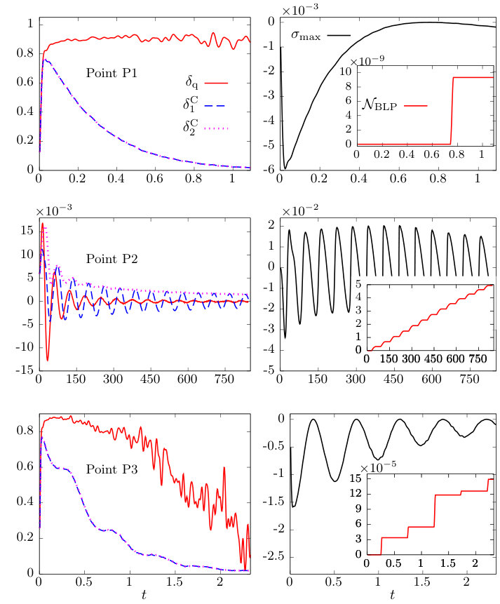 Figure 1
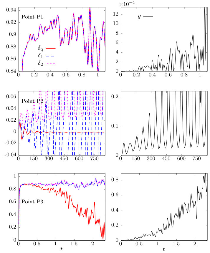 Figure 2
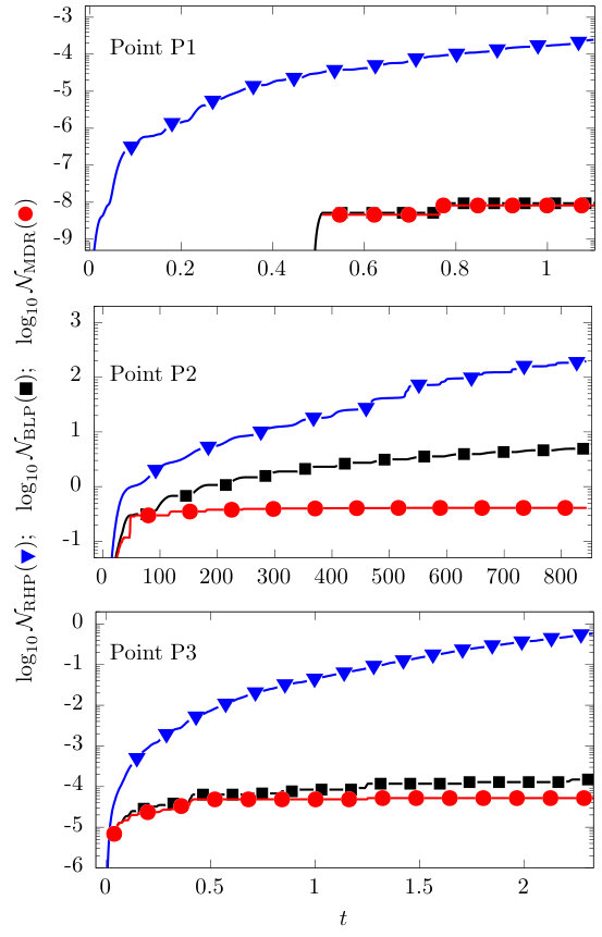 Figure 4
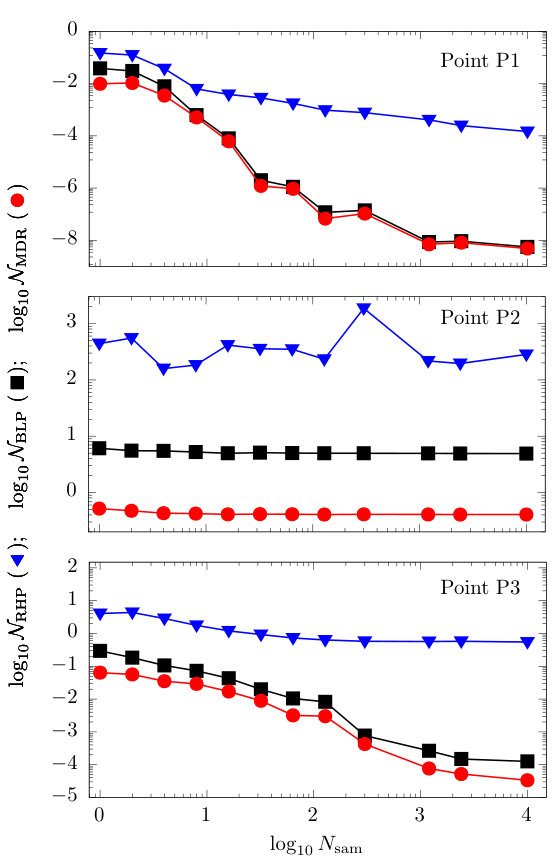 Figure 5
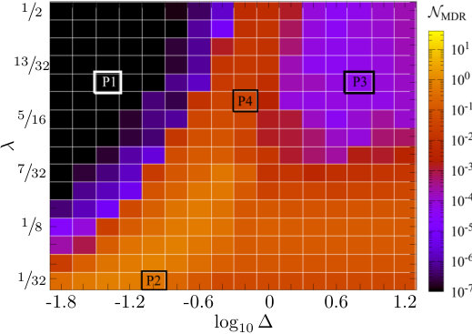 Figure 5
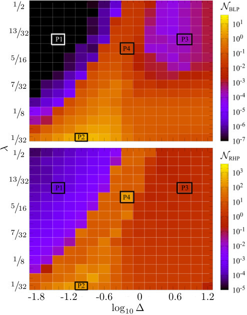 Figure 6
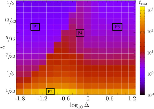 Figure 7
Peer Reviews
No public reviews on file for this paper yet. If you reviewed it on a platform where reviews are public (OpenReview, ICLR, NeurIPS, ICML), you can paste yours below so the community can read it here.
Videos
No videos yet. Explain this paper in a talk, walkthrough, or lecture? Add one.
Markovian and non-Markovian dynamics induced by a generic environment
M. Carrera
Instituto de Física, Benemérita Universidad Autónoma de Puebla, Apartado Postal J-48, Puebla 72570, México.
T. Gorin
Departamento de Física, Universidad de Guadalajara, Blvd. Marcelino García Barragan y Calzada Olímpica, Guadalajara C.P. 44840, Jalísco, México.
C. Pineda
Instituto de Física, Universidad Nacional Autónoma de México, México D.F. 01000, México
Abstract
We study the open dynamics of a quantum two-level system coupled to an environment modeled by random matrices. Using the quantum channel formalism, we investigate different quantum Markovianity measures and criteria. A thorough analysis of the whole parameter space, reveals a wide range of different regimes, ranging from strongly non-Markovian to Markovian dynamics. In contrast to analytical models, all non-Markovianity measures and criteria have to be applied to data with fluctuations and statistical uncertainties. We discuss the practical usefulness of the different approaches.
non-Markovianity, qubit, open quantum systems, random matrix theory
pacs:
03.65.Ud,03.65.Yz,03.67.Mn
I Introduction
Open quantum systems have been of interest for a long time Landau (1927). The interest stems from the natural separation of a quantum system into a central system of interest, and an uninteresting or uncontrollable part, usually denoted by environment. In 1967, Lindblad Lindblad (1976), Gorini, Kossakowski and Sudarshan Gorini et al. (1976) arrived at the so-called Lindblad master equation to describe the evolution of a central system weakly interacting with a memoryless environment. This equation has been of paramount importance in the field as one can, both, analytically solve several instances of the equation Prosen (2008), and describe accurately a wide range of experimental situations Carmichael (1999). The dynamics produced by such an equation is called quantum Markovian dynamics. Recently there has been an effort to classify and understand systematically open quantum systems which lie outside this description.
Definitions and measures for quantum non-Markovianity (NM) have received considerable interest in the last 10 years or so Breuer et al. (2009a); Rivas et al. (2010a). They are meant to characterize quantum processes (viz. the dynamics of open quantum systems) which cannot be described by a master equation with constant Lindblad operators. For such systems, there might be hierarchy of stronger/weaker non-Markovianity in the sense that it is easy/not-easy to describe the quantum channel by some effective evolution equation within the systems state space alone. A second quite different idea is that NM is a feature which might be taken advantage of in order to perform certain tasks. Both are valid points of view, but it is not clear to what extend some of the popular definitions and measures of NM provide relevant information with respect to these questions. Several reviews of the field can be found in Refs. Breuer (2012); Ángel Rivas et al. (2014); Breuer et al. (2016); de Vega and Alonso (2017).
Non-Markovianity has been studied extensively, for quantum processes with analytical solution, implying no fluctuations or uncertainties, applications to more realistic processes are relatively rare Liu et al. (2013); Urrego et al. (2018).
In the present paper, we study a quantum channel derived from the coupling of a two-level system to a “generic” quantum environment. We use random matrix theory (RMT) to describe that environment. Choosing the Hamiltonian in the environment from the Gaussian unitary ensemble (GUE), we find a variety of different behaviors in the relevant parameter space, ranging from Markovian (Lindblad-Dynamics) to strongly NM behavior. This model is ideal to discuss the questions raised above. Since the model has no known analytical solution, all criteria and measures must be calculated numerically, with unavoidable statistical errors, which resembles an experimental situation in which finite statistics come into play.
In Sec. II we present the model and find the structure of the quantum channel describing the dynamics of the system. In Sec. III, we introduce the NM measures, which we will use in Sec. IV for analysis. In Sec. IV we compare and interpret the different measures for the whole available region in the parameter space. We finish with some closing remarks in Sec. V.
II Model
The model to be used has been introduced in Ref. Carrera et al. (2014), which focussed on the derivation of an analytical description in the linear response regime. We find it suitable for the purpose of the present work, since it is a generic model, which, nontheless shows a broad range of different behaviors with respect to quantum NM. In this section, we describe the Hamiltonian of our system, and the quantum channel formalism used for a complete description of its dynamics.
II.1 The Hamiltonian
We consider a two level system (qubit) coupled to an environment. The Hilbert space of the qubit will be labeled by the subindex c and that of the environment by the subindex e. We assume that the dynamics in the whole Hilbert space is unitary, with the evolution governed by the Hamiltonian
[TABLE]
All subindices of operators in the right hand side indicate the subspace in which they act, except for , which is a Pauli matrix acting on the qubit. is the level splitting in the qubit and the parameter controls the strength of the coupling between the central system and the environment. The first two terms in Eq. (1) represent the free evolution of both central system and environment, while the third term provides the coupling which is assumed to be separable. The Hamiltonian of the environment shall be chosen from the Gaussian unitary ensemble to provide generality to the results discussed here Mehta (2004). We measure time in units of the Heisenberg time of and energy in units of the means level spacing in the center of the spectrum of ; in such units, . The density matrix of the central system for a time is given by
[TABLE]
where we have chosen a product state as the initial state of central system and environment. Just as , is also chosen from the Gaussian unitary ensemble, and the angular brackets denote an ensemble average over both random matrices. The magnitude of the matrix elements is chosen such that .
The most general form of has a parallel and perpendicular component, with respect to the internal Hamiltonian . If there is only a parallel component () the qubit dynamics becomes dephasing. The channel acting on the qubit can be obtained in terms of the fidelity amplitude for the Hamiltonians . This is already a very rich case; however, it has been considered before Gardiner et al. (1997); Gorin et al. (2004). The other limiting case is when the coupling is perpendicular to the internal Hamiltonian, which is the case we are studying here; see also Carrera et al. (2014). Thus we simply set, without loosing any generality,
[TABLE]
where is one of the three Pauli matrices.
II.2 Quantum channel formalism
We describe the reduced dynamics of the qubit with the quantum channel formalism, which means that the evolution of the system state is described in terms of a linear time dependent map acting on the space of density matrices of the central system. The map takes an arbitrary initial state, and returns the state evolved according to Eq. (2) for a time ,
[TABLE]
Since the image of this map is a density matrix, has two properties: (i) it preserves the trace of the argument and (ii) is completely positive. Maps with these characteristics will be referred to as quantum channels. We will also be interested in more general linear operators that preserve the trace but, even though map hermitian operators to hermitian operators, are not necessarily completely positive. In fact, we shall consider maps that are generally non positive. We will call such maps quantum maps. In this language, a quantum channel is a quantum map, but not necessarily the other way around.
A quantum map , and any linear map, is determined by its action on a basis; consider the computational basis and arrange the resulting elements in the matrix
[TABLE]
This is the so called Choi-matrix representation Choi (1975); Ziman and Heinosaari (2012). Since maps hermitian matrices to hermitian matrices, must also be hermitian.
It can be seen that the Choi matrix can be obtained by applying the extended map to a Bell state in the Hilbert space of two qubits:
[TABLE]
where . Thus, if is a quantum channel, is a two qubit density matrix, which in turn implies that , i.e. all of its eigenvalues must be positive or equal to zero.
We will now outline the procedure to construct the Choi matrix, based on the dynamics. The procedure will rely on two properties of our particular channel. First, it is unital, which means that the identity is mapped onto the identity. Second, the evolution of a diagonal operator remains diagonal, i.e. if is diagonal, so is in Eq. (4). The proof of both properties is found in the Appendix A. Let be the density matrices associated with the eigenvalues of the corresponding Pauli matrices. From the second property and trace conservation, we find that
[TABLE]
and from the first property, plus linearity of quantum maps, we get
[TABLE]
for some time dependent functions , and . From these equations, one can see that the dynamics in the axis is decoupled from the ones in the plane. If we define , we can write directly
[TABLE]
Notice that , and .
III Non-Markovianity measures
We consider NM as a property of a quantum process , which is a one-parameter family of quantum channels with and . The NM criteria and measures used here are based on two different concepts, (i) divisibility and (ii) contractivity. Both of them require knowledge of the intermediate quantum map
[TABLE]
In Appendix B.1, we calculate the Choi representation of this intermediate quantum map with the following result:
[TABLE]
with , , and . The parameters , and are the same as , and but calculated at a time . When or , is not invertible, and therefore may not exist.
III.1 Divisibility
A quantum process is divisible if and only if for any it holds that can be written as the composition , with being a valid quantum channel. Here, can be identified with the intermediate quantum map given in Eq. (10). Hence the divisibility of a quantum process is equivalent to all intermediate quantum maps being valid quantum channels. Formally speaking, the quantum process is divisible if and only if
- (a)
is invertible for almost all , and
- (b)
is a valid quantum channel if it exists.
In condition (a), we allow to be non-invertible at a finite (countable) number of points in time. In condition (b), we check the complete positivity of the intermediate map only for those , where is invertible.
RHP-Markovianity
One of the definitions of NM is given in terms of the divisibility of the quantum process under consideration. Following Rivas et al. Rivas et al. (2010b), we call a quantum process , RHP-Markovian if and only if the two conditions above are fulfilled.
To check for the complete positivity of the intermediate quantum map, Rivas et al. consider the trace norm of the associated Choi matrix defined as , where are the eigenvalues of . Since the sum of the eigenvalues always is equal to the dimension of the Hilbert space of the physical system, due to trace preservation, any negative eigenvalue will necessarily lead to being larger than two. In addition, since the composition of two quantum channels is again a quantum channel, it is sufficient to check complete positivity for infinitesimal , only. Hence, Rivas et al. define the function
[TABLE]
which is zero if the intermediate map is completely positive, and greater than zero otherwise. Moreover, to define a measure of the degree of non-Markovianity of the process, the authors integrate this function over time. We shall label this quantity as
[TABLE]
Notice that if and only if the process is divisible for all times up to .
Application to our model
In order to check the RHP-Markovianity (divisibility) of as defined in Sec. II, we use the Choi representation, Eq. (11) of the intermediate quantum map . The eigenvalues of are
[TABLE]
Hence, the eigenvalues are non-negative if and only if (i) and (ii) .
Since we can limit to infinitesimal , we expand the different functions in Eq. (11) around and obtain, to first order,
[TABLE]
where we have used the fact that , , and .
The two conditions (i) and (ii) can now be written as
[TABLE]
where we introduced
[TABLE]
Additionally we used the fact that for any complex number , on the expression for . Finally, we combine the two inequalities into
[TABLE]
We can now relate our inequalities to the criterium of Rivas et al. as follows. In our case, the trace norm of the Choi matrix, can be written as
[TABLE]
This yields
[TABLE]
We showed that non-negativity of the eigenvalues is equivalent to the double inequality . Then we saw that it is also equivalent to . This means that the double inequality holds if and only if .
III.2 Contractivity
Markovianity of classical stochastic processes imply that probabilities distributions decrease their Kolmogorov distance with time van Kampen (2007). This is interpreted as a loss of information of the initial conditions. Carrying this ideas to a quantum level results in a definition of Markovianity Breuer et al. (2009b). Let denote the evolution of two states . We define
[TABLE]
where is the trace distance, which is directly related with the probability of distinguish the state from the state , i. e., it is their distinguishability Nielsen and Chuang (2000), and . In other words, is the derivative of the distance between the evolved states. We say that a process is contractive if for all and all , we have that . A process is said to be non-Markovian if it is not contractive. Breuer et al. then define the following quantity as a measure for the degree of non-Markovianity:
[TABLE]
The calculation of this measure is greatly simplified when the process acts on a qubit. To perform this maximization, one should consider only pure, orthogonal initial states Wißmann et al. (2012). Indeed, we found that only depends on the vector difference between the representations of initial states in the Bloch ball (see Appendix B.2). Moreover, the distance between the two points representing the initial states enters as a homogeneous scale factor. It therefore possible, restricting the maximum search to such cases, where is a pure state, and the uniform mixture. If the pure state is parametrized in spherical coordinates by the angles and , we obtain [cf. Eq. (65)]
[TABLE]
with .
In what follows, we derive a criteria for NM based on the contractivity, which can be compared to the criteria Eq. (21) obtained in Sec. III.1, based on divisibility. Since may be chosen freely in Eq. (26), a given process is Markovian in the sense of Breuer et al., if and only if both functions, and are non-increasing at all times. In other words if
[TABLE]
for all times. Condition (27) becomes which in turn is equivalent to (at least as long as , i.e. away from the points where is not invertible). To consider condition (28), we expand as
[TABLE]
where , and . Setting and , we may write
[TABLE]
From this, it is clear that the largest time derivative of is . With , we find and such that
[TABLE]
To summarize, for the process to be Markovian (in the sense of contractivity), it is required that both, and . This is equivalent to
[TABLE]
where
[TABLE]
This double inequality is the analog of Eq. (21), which has been derived as criterium for Markovianity in the sense of divisibility.
For unital maps like the one considered here, contractivity of the trace distance can be identified with positivity. That means that our quantum process is contractive if and only if all intermediate maps are positive. Note that divisibility is defined as all intermediate maps being completely positive. Thus, there may be processes which are contractive but not divisible Chruściński et al. (2011). Therefore, we may find regions in the parameter space of our system, where the dynamics is contractive (i.e. BLP-Markovian) but not divisible (i.e. RHP-Markovian). A recent, comprehensive discussion on different criteria for divisible and contractive processes can be found in Ref. Cabrera et al. (2019).
III.3 Maximal recovery
This quantifier of non-Markovianity can be based on any capacity-like property of the channel. In fact, we use distinguishability, maximized over states, just as the BLP-measure. However, instead of summing up all the small increments, we search for the maximum distinguishability recovery over the whole quantum process Pineda et al. (2016):
[TABLE]
where is defined in the text below Eq. (24). The BLP-measure has been related to the backflow of information, which can be quantified indeed in terms of the recovery of distinguishability. However, in order to quantify the amount of information recovered, it is much more sensible to use , than integrating over all backflow in a process, where information is fluctuating back and forth between system and environment. Of course there is a price to pay. It is quite more expensive to compute , than it is to compute , because of the additional degrees of freedom, and .
IV Numerical simulations
In this section, we apply different methods to characterize the (non-)Markovian dynamics of a generic open quantum system. The quantum process to be studied is obtained by numerical simulations of the Hamiltonian in Eq. (1) with the initial state of the environment taken as the maximally mixed state. This includes a Monte-Carlo sampling of a random matrix ensemble. Therefore, the numerical data are contaminated by residual statistical fluctuations due to the finite size of the sample. We stress that residual fluctuations would be present, in experimental situations, also. The dimension of the Hilbert space of the environment is set to and the sample size is fixed to unless otherwise stated.
In our model system, defined in Eq. (1), we can identify three different energy scales. The average level spacing in (which is set equal to one), the spacing between the two levels of the qubit, and the coupling strength between qubit and environment. In an effort to explore the properties of our model as thoroughly as possible, we consider a rectangular region in the parameter space . For , the interesting range reaches from values much smaller than the mean level spacing to values much larger, thus we choose the limits , covering a range of three orders of magnitude. For , we choose the lower limit where is much smaller than the average level spacing in , such that perturbation theory would be applicable for the Hamiltonian . The upper limit, by contrast, is dictated by the requirement that our model reproduces the behavior of the random matrix model in the limit , in such a way that finite size effects are still negligible. For that to hold, the spreading of eigenstates of expanded in the basis of must be small compared to the spectral range of . Both considerations lead us to the limits . A similar parameter range has been explored in Ref. Carrera et al. (2014).
In order to obtain reliable values for the two measures, we establish a finite ending time for the processes to be studied. At that time, the system will have relaxed so much that the remaining dynamics is unusable for any practical purposes. Our approach for finding a sensible definition for the ending time is described in Sec. IV.1. In Sec. IV.2 we present and discuss the results for three non-Markovianity measures. Moreover we select several representative parameter sets that are analyzed in detail in Sec. IV.3. In particular, we study the dependence of the measures on the number of samples considered. The motivation is to understand the statistical significance of the results presented in Sec. IV.2. At the end, this could be useful for identifying a NM measure which is accurate, robust and significant. We finish this section by analyzing the local (in time) criteria for non-Markovianity in Sec. IV.4. We consider divisibility and contractivity, via the corresponding inequalities Eq. (21) and Eq. (32). Both conditions are tested for the infinitesimal intermediate quantum map as defined in Eq. (10), and examine carefully the usefulness of such kind of expression under statistical fluctuations.
IV.1 Process ending time
For the NM measures to be considered below (Sec. IV.2) it is essential to define an ending time for the quantum process in question. However, two conflicting requirements arise. On the one hand the ending time should be sufficiently large, such that the dynamics of the process is completely contained, but on the other hand it should also be sufficiently short, such that the contaminating contribution from residual statistical fluctuations remain small.
The quantum process studied here, has the convenient property that if one chooses as initial state an eigenstate of , the system converges to the uniform mixture in the limit of long times. Along this process, the purity decays from to . We choose the ending time for the process at that time, where the purity of is equal to , which means that the purity has decayed to above its minimum value. Of course other values of the same order are equally possible, but they do not change the general results of our study.
In Fig. 1 we show the process ending time as a function of the parameters and , color coded over the parameter space. While we use a linear scale for , is varied on a log-scale. The resulting ending time varies over several orders of magnitude, so we also use a log-scale for the color mapping. While increases, the becomes smaller exponentially fast, since for large , the Fermi golden rule approximation applies Carrera et al. (2014). It is however quite remarkable that for small , the largest can be found near , which is approximately equal to , where is the Heisenberg time in the random matrix environment. In other words, at the period of the Rabi oscillation is equal to the Heisenberg time.
For all non Markovianity measures we choose unless otherwise stated, and we shall thus drop the time dependence.
IV.2 Three measures for non-Markovianity
Analyzing Fig. 2, we find that both measures reach smallest values in the upper left corner of the parameter space, shown. Indeed, due to the following argument, we expect the quantum process to be at least close to Markovian in this region. The standard prescription for deriving a quantum master equation via the Born-Markov approximation consists in the following steps Breuer and Petruccione (2002): (i) Couple the central system weakly to each of the many degrees of freedom in the environment (Born approximation), (ii) let the number of degrees of freedom in the environment go to infinity, and (iii) assume the environment correlation functions to decay almost instantaneously on the time scale of the reduced dynamics (Markov condition). In terms of level density and average local level spacing, condition (i) and (ii) lead to a wide range in energy with an exponentially high level density, which means that the perturbation strength will be large as compared to the level spacing. This regime is known as the Fermi-golden-rule regime Merzbacher (1998). Note that in this parameter region, , which results in a slow system dynamics so that condition (iii) is fulfilled.
By contrast, for sufficiently small coupling and not too small , the dynamics is clearly NM. It is clear that in this region at least some of the conditions mentioned above are not fulfilled. The region of strongest NM behavior is around and small values of .
An interesting area is in the upper right region of the NM maps in Fig. 2. There, the BLP measure of Eq. (25) tends to very small values, while the RHP measure, Eq. (13), remains constant. As explained at the end of Sec. III.2, the RHP criterion is more restrictive than the BLP criterion, as it requires complete positivity and not just positivity for the intermediate maps. It is thus possible that a given quantum process is BLP-Markovian but not RHP-Markovian. Due to residual statistical fluctuations, a definite judgement is difficult.
Fig. 3 shows as defined in Eq. (34) up to the ending time as a function of and . Its behavior is more similar to than to , which may be related to its common origin. Note though that the boundary between the regions of Markovian and strongly non-Markovian behavior is sharper. The region of strong NM is also somewhat larger, located in an area parallel to the M-NM boundary, at values for below , of about 12 blocks in size. Finally, note the region in the upper right corner. There, the MDR measure leads to (relatively) lower values than the BLP measure, in distinction to the RHP measure which reaches much larger values.
IV.3 Robustness and convergence of the NM measures
In the previous section, we presented the results of three different measures for NM. For our model, we found a wide range of different behavior, depending on the choice of the parameters, and . Here, we study the robustness and accuracy of the measures in more detail. For that purpose we select three points in parameter space, where the behavior of the quantum process is quite different:
- •
Point P1 (), where the dynamics is Markovian, or at least very close to it.
- •
Point P2 (), where it is maximally non-Markovian – according to the BLP-measure.
- •
Point P3 (), where the dynamics looks like being more NM according to RHP than according to BLP or MDR – compare the two heat maps in Fig. 2.
Finally, we select a additional fourth point for a later remark:
- •
Point P4 ().
Let us now discuss the numerical results. In Fig. 4, the NM-measures are shown as a function of time. In other words, we compute the NM-measures as if the quantum process would end at time , instead of . It is clear from the definition of all three measures, that they must be monotonously increasing: whenever .
For P1 (Markovian point; top panel), the RHP-measure (blue line, triangles) increases continuously with time – even though it always remains rather small. The other two measures by contrast show only one increment at and afterwards remain approximately constant around a value of . This makes it difficult to decide unambiguously whether the process is Markovian or non-Markovian.
For P2 (strongly NM; middle panel), the RHP-measure increases to very large values of the order of . The BLP measure also increases along the full time range up to values of the order , while the MDR measure quickly saturates at a value of the order of (note that the MDR measure is by definition limited to values below one). The different behavior between BLP and MDR will be discussed below, where we consider the criteria for contractivity. In any case, all three measures clearly show the NM of the process.
For P3 the RHP-measure increases continuously as in the previous cases, reaching values of the order of . By contrast, the other two measures, BLP and MDR remain below a value of the order of . This may hint towards the possibility that here, the quantum process is P-divisible but not CP-divisible.
In Fig. 5, we plot the NM-measures versus the sample size, , where we expect that the NM-measures approach a limit value for , the true ensemble average. For point P1 (top panel), as the ensemble size increases, all measures tend algebraically to zero. For point P2 (middle panel) all measures converge to a finite values, whereas for point P3, the measures based on distinguishability seem to drop to zero while the one based on divisibility attains a finite value. In other words, this result suggests that the dynamics is P-divisible but not CP-divisible at that point Chruściński et al. (2011).
Environment size
We also experimented with different environment sizes, but the results did not change significantly. In fact, it can be shown that this may have an effect at short times only; in general, one would expect finite size effects of at times of the order of in units of the Heisenberg time. These are not our concern, since we define our model in the limit .
Non-equivalence of NM measures
A second interesting question is that of “quantitative equivalence”. Two measures for a physical property may be called (quantitatively) equivalent, if and only if
[TABLE]
for any two states of some system. For example, if one thermometer (calibrated according to the empirical temperature ) finds that a body is colder than a body , any other thermometer (calibrated according to some different empirical temperature ) should find the same relation. Analyzing carefully our results in Fig. 2, we can indeed find pairs of points in parameter space, where the two NM-measures and violate this condition. For instance, is clearly larger at P4 than at P2, while in the case of it is just the other way round.
IV.4 Time evolution of Markovianity criteria
Here, we study the behavior of the two time-local criteria for non-Markovianity which are based on divisibility and contractivity, described in Sec. III.
For the divisibility, we consider the requirements given in Eq. (21) on the one hand, and the condition with given in Eq. (12). While formally, both criteria are equivalent [see Eq. (23)], we will see that in the presence of experimental/statistical uncertainties, one might be easier to verify than the other. In Fig. 6 we present the aforementioned expressions for points P1, P2 and P3 for times ranging from zero to .
For point P1 (top two panels), we see that the inequalities are saturated, in the sense that are apparently all equal. Despite that, the function is not identically equal to zero, however it is small. The inequalities have allowed to correctly identify the point as Markovian, in agreement with the analysis of Fig. 5. In fact, for larger ensemble sizes the value of diminishes.
The behavior of and for point P2 can be seen in the middle panels of Fig. 6. Here, the different curves corresponding to cross each other in a systematic and ordered fashion, indicating non-Markovianity beyond statistical fluctuations. This is also seen in the behaviour of the corresponding , which oscillates regularly around values of the order of . Notice that we identified this point as displaying non-Markovian behavior, again with the aid of Fig. 5.
Finally, point P3 is studied in the lower panels of Fig. 6. We can see that the curve corresponding to is not between the ones corresponding to . The conclusions are confirmed by the behavior of , where one finds notorious fluctuations on top of a smooth curve which increases systematically as a function of time. Thus, according to the divisibility criterion, the system is non-Markovian, as concluded from the lower panel of Fig. 5.
In the case of the Markovianity measure based on the contractivity of the process, the condition translates to Eq. (32) for the channels here considered, see Eq. (9). For a given time , a certain initial pair of states will yield the maximum as defined in Eq. (25). For these states, one can calculate
[TABLE]
and see how the final value of the measure is built with time. Notice that is different from the derivative of , recall Eq. (25), as for each ending time , the states that maximize the quantifier are different, whereas in Eq. (35) we fix the ending time; however, for equal to the ending time, they coincide.
On the top left panel we can see that Eq. (32) is apparently fulfilled during the whole process, however, since the two curves for and lie on top of each other, the inequality might be violated on a smaller scale. On the top right panel, we see that indeed the measure is close to zero; for it is numerically zero, and afterwards, close to . From this evidence, we arrive at the conclusion that the point is Markovian, with respect to contractivity, in agreement with the same case studied in Fig. 6.
The point P2 is analyzed in the middle panels. The function oscillates around zero with decreasing amplitude, while provides an upper bound for . Indeed, whenever this bound is saturated, has an node, and has a minimum, making the system “very Markovian”. On the other hand, when the difference between and is largest, has a maximum, and the system becomes very non-Markovian. Thus, as can be seen on the right, oscillates regularly and with a relatively high amplitude around zero. The NM measure, adds up the areas below the positive parts of , which we expect to have a similar behavior as , shown here. Therefore, the point P2 shows a genuine non-contractive behavior and the dynamics is NM in this case.
The point P3 is analyzed in the bottom panels. All three functions and display a similar behaviour as for point P1, but for we observe stronger statistical fluctuations. In this case, however, oscillates, and has a maximum in 0. The measure picks up small statistical fluctuations which diminish as we increase the sample size and may therefore be regarded as spurious. We can conclude that the process for point P3 is contractive, in agreement with previous conclusions.
The criteria provided in Eqs. (21) and (32), indeed provide a usefull tool to understand if a certain non-zero value for one of the NM measures should be regarded as statistically significant or not. In some cases it is helpful to analyze the behavior of the measures under variation of the sample size in order to arrive at the correct decision.
V Conclusions
In this article we studied a qubit coupled to a generic environment modeled by random matrices. The model Hamiltonian contains a factorizable interaction between qubit and environment, and provides the qubit with an internal dynamics perpendicular (in the Bloch representation) to the one induced by the interaction. This induces a channel structure for which we were able to derive analytical conditions for several criteria of Markovianity. In spite of its simplicity, the model displays rich dynamics in the qubit, beyond pure depolarization or dephasing.
We then applied the criteria to determine for which parameters the model yield Markovian dynamics in the qubit. We found several difficulties with verifying Markovianity criteria for the numerical data, which we expect to appear also in real experimental situations. Fluctuations due to noise, and/or due to finite sample sizes may contribute notably to the finite value of a non-Markovianity measure and thereby suggest non-Markovian behavior, whereas the clean system really is Markovian. An analysis like the present one, where the ensemble size is increased such that residual fluctuations diminish, eventually reveals the true behavior.
Acknowledgements– Support by projects CONACyT 285754, UNAM-PAPIIT IG100518, Benemérita Universidad Autónoma de Puebla (BUAP) PRODEP 511-6/2019-4354 and CONACyT 220624-CB are acknowledged
Appendix A Born series
In this section, we prove that the quantum channel, describing the dynamics of the qubit under coupling to the RMT environment, has the form of a X-state Roa et al. (2014) as postulated in Eq. (9). For doing so, we use the entire expansion of the evolution of system and environment in a Born series. We consider the more general case of an arbitrary mixed initial state in the environment, and only at the end specialize to the case .
In the interaction picture, a solution to the Hamiltonian
[TABLE]
may be written as
[TABLE]
Here, we stick to the convention chosen in the main part of this paper, where the time variable measures time in units of the Heisenberg time, which results in . The echo-operator describes the evolution of the state , such that . In the original Schrödinger picture, it thus holds:
[TABLE]
As a formal solution of the evolution equation in the interaction picture, the echo operator fulfills the following integral equation
[TABLE]
Here, the second line represents the afore mentioned Born series, where the interaction has been written in block-matrix notation:
[TABLE]
Here, we will calculate the average of , with respect to the random matrix ensemble for . This defines the quantum map as
[TABLE]
and thereby its Choi-matrix representation, in Eq. (9). Below, we will also consider this quantum map in the interaction picture, defined as
[TABLE]
Simplified notation
For our purpose, it is convenient to introduce the following more compact notation for the multi-dimensional time integrals:
[TABLE]
Note that we enumerate the different time variables from smallest to largest starting at the time closest to zero. Next, we will introduce an independent notation for the integrands. Let us consider the caso of an even number of product terms, first:
[TABLE]
since is Hermitian. Note that the product terms on the LHS of the first equation, must be ordered according to decreassing time arguments, just as in Eq. (36). From an explicit computation we find
[TABLE]
Note that the product terms must be ordered such that time increases from right to left. For an odd number of terms:
[TABLE]
With this, we may write for the echo operator
[TABLE]
Ensemble averaged quantum channel
Averaging over the random matrix implies that only such terms survive, which contain an even power of matrices and . This means that the indices of summation must either be both even or both odd. Therefore,
[TABLE]
For the quantum channel in the interaction picture, Eq. (38) it is now easily verified that
[TABLE]
This and Eq. (37) then show that is indeed of the form postulated in Eq. (9), and it yields the following expressions for :
[TABLE]
The second equation results from the fact that the reduced evolution of the qubit conserves the trace. Naturally, it is difficult to prove this directly, from the expressions derived here. Let us now consider . In this case, as in the previous one, , and we find
[TABLE]
Again, the resulting qubit state is diagonal, however unless we specialize to the case , the function is different from corresponding to the previous case.
[TABLE]
We continue with the off-diagonal blocks of the Choi-matrix representation of the quantum channel:
[TABLE]
This result confirms again the general X-state structure of the Choi-representation of our quantum channel. In terms of the parametrization in Eq. (9), we find:
[TABLE]
where the phases arise from returing to the Schrödinger picture, according to Eq. (37). Finally,
[TABLE]
For any Hermiticity conserving linear map, the Choi-representation itself must be Hermitian, in particular also for our quantum channel, as can be seen from its definition in terms of the reduced dynamics in Eq. (2). This implies that
[TABLE]
In the case of the equivalence of the Eqs. (50) and (52) is rather obvious. One simply has to exchange the variable names and along with and . In the case of , we do not see any simple way of proving the equivalence in terms of the present approach.
Collecting results for the case
From the considerations in the previous paragraph, we found that the Choi-matrix representation of the quantum channel defined by the Eqs. (2) and (37) is given by
[TABLE]
The general X-state structure (i.e. all the zeros in this matrix) follows directly from the considerations in this section. For simplicity we omitted the time argument in this representation. The functions , , , and are as defined above. Some of the dependencies between these matrix elements could not be proven within our derivation, but are valid due to elementary properties of the evolution equation (2). This is the case for trace conservation (diagonal blocks) and Hermiticity (off-diagonal blocks).
As a last point, we show that for , it holds that . In this case, and for , we find from Eq. (2):
[TABLE]
This means that no matte if we perform an ensemble average or not, the resulting quantum channel is unital (it maps the identity onto itself). This in turn implies:
[TABLE]
Appendix B Two representations of a quantum channel
We will use two different representations. (i) The “super operator” representation which is nothing else than the standard matrix representation of a linear map on a vector space. This representation is easy to read directly from the evolution of a standard set of states; in fact, we shall construct it in that way. (ii) The Choi-matrix representation in which verifying inherent quantum channel properties is easier.
For the super operator representation, we represent the density matrices as column vectors, in the so-called “anti-lexicographical” ordering Bengtsson and Zyczkowski (2006). For a single qubit, we have
[TABLE]
This fixes the matrix representation of the map , since the columns of must be the images of the canonical basis vectors. Thus, with the condensed form , we obtain
[TABLE]
The super operator representation has the convenient property, that the representation of the composition of two quantum maps, (where is applied to the result of ) is simply given by the matrix product of the representations and of the individual maps: .
B.1 Quantum map for intermediate time steps
We know that the superopertor has the following form
[TABLE]
where and are functions on time.
For given quantum maps and , we compute the quantum map which takes states form time to . For the moment we assume to be finite. The central question is whether is a CP-map, or not. While the super-operator representation is appropriate to compute the composition of and , the Choi representation is needed for verifying the complete positivity. From given on (57) of the section II we have its inverse matrix
[TABLE]
where and .
If we denote with primes the functions evaluated on , that is, similarly for and , then
[TABLE]
We found that the super-operator representation corresponding to is given by
[TABLE]
where and . The corresponding Choi matrix turns out of reshuffle the above matrix:
[TABLE]
on subsection III.1 the divisibility of is explored via the positivity (non negative eigenvalues) of Choi matrix .
B.2 Trace distance and contractivity
We have introduced the trace distance and its definition through of the eq. (24). Furthermore, turns out that the trace distance of an Hermitian matrix is equal to one half of the sum of absolute values of its eigenvalues.
Given two any states and which evolve under the quantum channel , its trace distance at the time can be calculate as
[TABLE]
the right side of above equation follows from the linearity of and due that . Now, if the states and are described by the Bloch vectors and , respectively. We can write down
[TABLE]
where the are the vector components of . Using the linearity of and spherical coordinates for we have
[TABLE]
which is an Hermitian matrix therefore
[TABLE]
The reference list from the paper itself. Each links out to its DOI / PubMed record.
- 1Landau (1927) L. Landau, Zeitschrift für Physik 45 , 430 (1927).
- 2Lindblad (1976) G. Lindblad, Communications in Mathematical Physics 48 , 119 (1976).
- 3Gorini et al. (1976) V. Gorini, A. Kossakowski, and E. C. G. Sudarshan, Journal of Mathematical Physics 17 , 821 (1976).
- 4Prosen (2008) T. Prosen, New Journal of Physics 10 , 043026 (2008).
- 5Carmichael (1999) H. Carmichael, Statistical Methods in Quantum Optics 1: Master Equations and Fokker-Planck Equations , Physics and Astronomy Online Library (Springer, 1999), ISBN 9783540548829.
- 6Breuer et al. (2009 a) H.-P. Breuer, E.-M. Laine, and J. Piilo, Phys. Rev. Lett. 103 , 210401 (2009 a).
- 7Rivas et al. (2010 a) Á. Rivas, S. Huelga, and M. Plenio, Phys. Rev. Lett. 105 , 050403 (2010 a).
- 8Breuer (2012) H.-P. Breuer, Journal of Physics B: Atomic, Molecular and Optical Physics 45 , 154001 (2012).