The angular scale of homogeneity in the Local Universe with the SDSS blue galaxies
F. Avila, C. P. Novaes, A. Bernui, E. de Carvalho, J. P., Nogueira-Cavalcante

TL;DR
This study measures the angular scale at which the local Universe appears homogeneous using SDSS blue galaxies, confirming consistency with other tracers and supporting the Cosmological Principle within the ΛCDM model.
Contribution
It provides the first precise measurement of the angular homogeneity scale using SDSS blue galaxies and compares it with HI sources, validating the homogeneity transition in the local Universe.
Findings
Angular homogeneity transition at ~22°
Results consistent with ALFALFA HI sources
Supports ΛCDM predictions and the Cosmological Principle
Abstract
We probe the angular scale of homogeneity in the local Universe using blue galaxies from the SDSS survey as a cosmological tracer. Through the scaled counts in spherical caps, , and the fractal correlation dimension, , we find an angular scale of transition to homogeneity for this sample of . A comparison of this measurement with another obtained using a different cosmic tracer at a similar redshift range (), namely, the HI extragalactic sources from the ALFALFA catalogue, confirms that both results are in excellent agreement (taking into account the corresponding bias correction). We also perform tests to asses the robustness of our results. For instance, we test if the size of the surveyed area is large enough to identify the transition scale we search for, and also we…
Click any figure to enlarge with its caption.
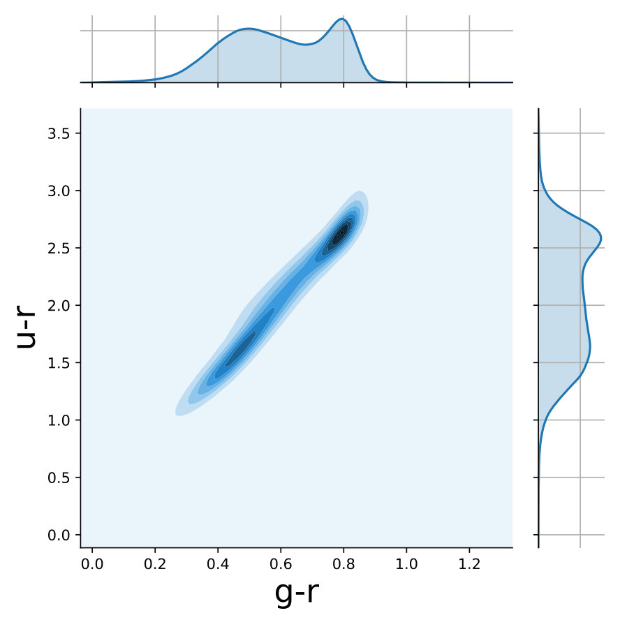 Figure 1
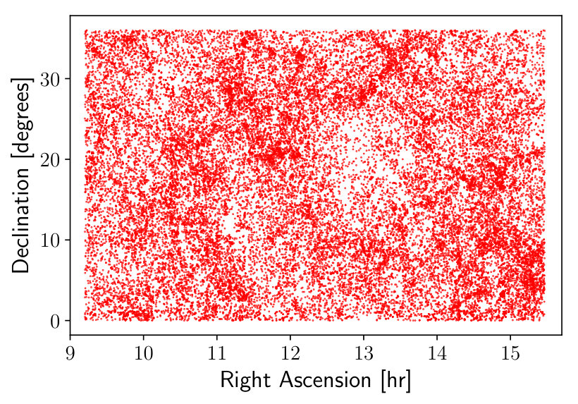 Figure 2
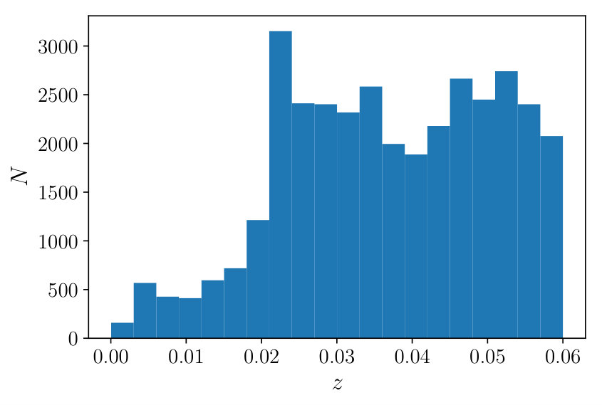 Figure 3
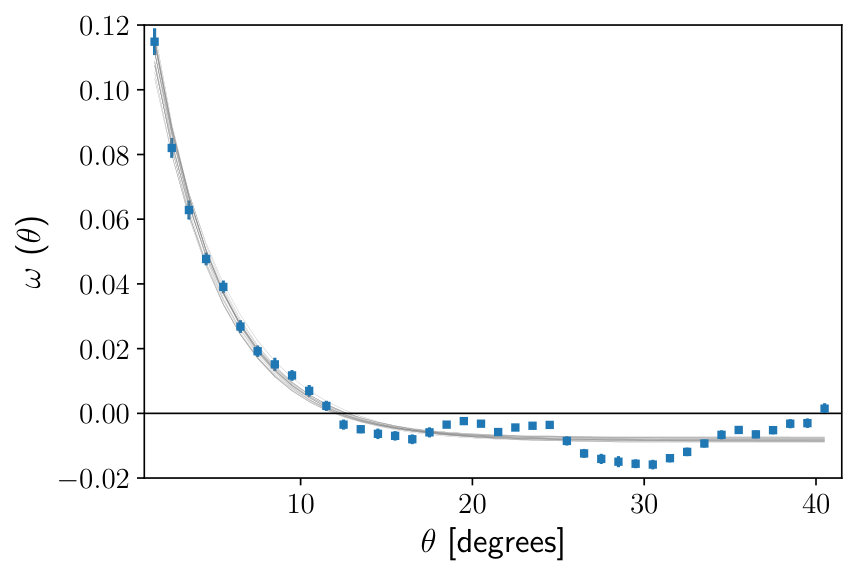 Figure 4
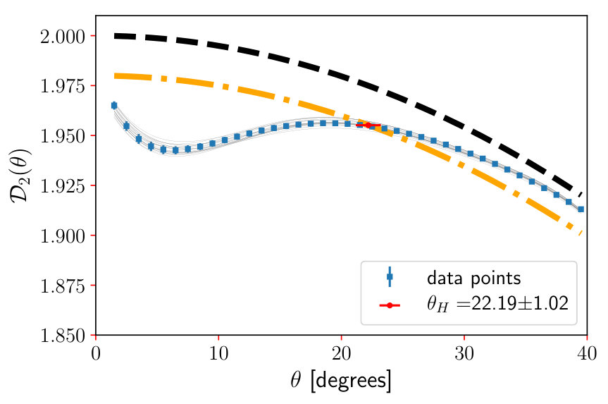 Figure 5
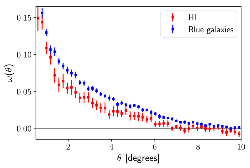 Figure 6
 Figure 7
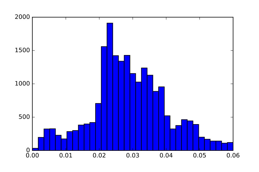 Figure 7
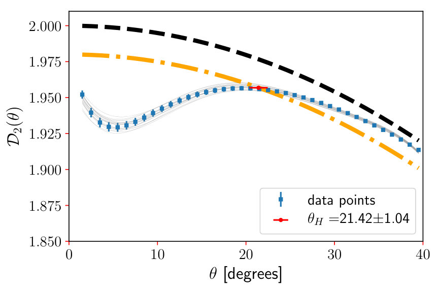 Figure 7
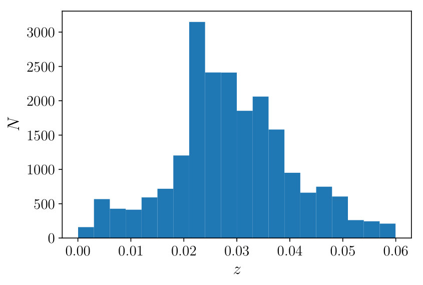 Figure 8
 Figure 8
| SDSS blue gals. | ALFALFA HI | ALFALFA HI | theoretical | ||
| measured | measured | measured | bias corrected | prediction | |
Peer Reviews
No public reviews on file for this paper yet. If you reviewed it on a platform where reviews are public (OpenReview, ICLR, NeurIPS, ICML), you can paste yours below so the community can read it here.
Videos
No videos yet. Explain this paper in a talk, walkthrough, or lecture? Add one.
The angular scale of homogeneity
in the Local Universe with the SDSS blue galaxies
F. Avila,1 C. P. Novaes,1 A. Bernui,1 E. de Carvalho,1,2 J. P. Nogueira-Cavalcante1
1Observatório Nacional, Rua General José Cristino 77, São Cristóvão, 20921-400 Rio de Janeiro, RJ, Brazil
2Centro de Estudos Superiores de Tabatinga, Universidade do Estado do Amazonas, 69640-000, Tabatinga, AM, Brazil e-mail: [email protected]
(Accepted XXX. Received YYY; in original form ZZZ)
Abstract
We probe the angular scale of homogeneity in the local Universe using blue galaxies from the SDSS survey as a cosmological tracer. Through the scaled counts in spherical caps, , and the fractal correlation dimension, , we find an angular scale of transition to homogeneity for this sample of . A comparison of this measurement with another obtained using a different cosmic tracer at a similar redshift range (), namely, the HI extragalactic sources from the ALFALFA catalogue, confirms that both results are in excellent agreement (taking into account the corresponding bias correction). We also perform tests to asses the robustness of our results. For instance, we test if the size of the surveyed area is large enough to identify the transition scale we search for, and also we investigate a reduced sample of blue galaxies, obtaining in both cases a similar angular scale for the transition to homogeneity. Our results, besides confirming the existence of an angular scale of transition to homogeneity in different cosmic tracers present in the local Universe, show that the observed angular scale agrees well with what is expected in the CDM scenario. Although we can not prove spatial homogeneity within the approach followed, our results provide one more evidence of it, strengthening the validity of the Cosmological Principle.
keywords:
Cosmology: Observations – Cosmology: Large-Scale Structure of the Universe
††pubyear: 2015
1 Introduction
In few years cosmology has achieved an unprecedented level in the restriction of parameters of the most reliable cosmological models due, mainly, to the high quality of observational data and to the diversity of cosmic tracers observed (Aghanim et al., 2018; Abbott et al., 2018; Alam et al., 2017). Nowadays, these data is being used to test the Cosmological Principle (CP), the main hypothesis that supports the concordance model of cosmology.
The statistical isotropy of the universe is being tested for many extragalactic objects like Radio sources (Blake & Wall, 2002; Ghosh et al., 2016), Gamma-ray bursts (Bernui et al., 2008a; Tarnopolski, 2017; Řípa & Shafiello, 2018), galaxy clusters (Bengaly et al., 2017a), and galaxy datasets like the WISE (Yoon et al., 2014; Bengaly et al., 2017b; Novaes et al., 2018) and the SDSS catalogues (Sarkar et al., 2019), where all these analyses show a good concordance with the isotropy of the universe. The Planck Convergence and Cosmic Microwave Background temperature fluctuations maps have been examined and are also consistent with statistical isotropy at small angular scales (Ade et al., 2016; Novaes et al., 2016; Marques et al., 2018), although some controversy remains at large angles (Bernui, 2008b; Gruppuso et al., 2013; Polastri, Gruppuso & Natoli, 2015; Schwarz et al., 2016; Aluri, Ralston & Weltman, 2017; Rath et al., 2017; Bernui et al., 2018).
The study of spatial homogeneity using datasets is more recent, and is a delicate issue. Methods that explore the homogeneity of the matter distribution counting objects in spheres or spherical caps (in case the objects are projected on the sky) are not direct tests of spatial homogeneity because the counts are restricted to the intersection of the past light-cone with the spatial hyper-surfaces (see, e.g., Ellis, 2006; Maartens, 2011). Rigorously, these methods provide consistency tests in the sense that: if the counting methods shows that the objects distribution does not approach homogeneity on any scale, then this can falsify the CP. On the other hand, if data confirm the existence of a transition scale to homogeneity, then this strengthens the evidence for spatial homogeneity, but does not prove it (Maartens, 2011).
To investigate homogeneity in a given sample, one searches for a characteristic scale, , beyond which the distribution of cosmic objects can be considered homogeneous. In the counts-in-spheres method, one averages the number of objects inside spheres of radius , , and take their logarithmic derivative to obtain the fractal correlation dimension, (Scrimgeour et al., 2012). For a homogeneous distribution of objects, one should expect a behaviour like , with at small scales, , and at larger sphere radius, (Castagnoli & Provenzale, 1991; Sarkar & Pandey, 2018). However, this method does not deal correctly with incomplete catalogues and boundary effects; remember that often the astronomical data is located in disconnected sky patches, with contours that are not straight lines, and may contain holes due to the application of masks. To solve these inconveniences, Scrimgeour et al. (2012) introduced the scaled counts-in-spheres method, which consists of taking a normalised ratio of counts, considering the data and simulated homogeneous samples. This method and the equivalent quantity adapted to a 2-dimensional (2D) analysis, the scaled counts-in-caps (or spherical caps), have been applied to study homogeneity in several catalogues [Nadathur (2013); Laurent et al. (2016); Pandey & Sarkar (2015); Sarkar et al. (2016); Ntelis et al. (2017); Gonçalves et al. (2018a, b); for a different approach see, e.g., Hoyle et al. (2013)].
The present work analyses the clustering features of the current sample of blue galaxies from the Sloan Digital Sky Survey (SDSS). The three main objectives of doing so, are:
(i) to study if an angular scale of transition to homogeneity can be revealed by the SDSS blue galaxies in the local Universe;
(ii) to find the relative bias between two cosmic tracers (at similar redshift): the HI sources from the ALFALFA catalogue and the SDSS blue galaxies, ;
(iii) to confirm if the scale found in (i) equals –considering the relative bias– the angular scale of homogeneity in the local Universe recently found by Avila et al. (2018) using the ALFALFA catalogue (homogeneity scales obtained in two samples can be compared if one knows the relative bias; see, e.g., Scrimgeour et al., 2012; Ntelis et al., 2017).
Our work is organised as follows. In section 2 we present the selection of the data. In section 3 we describe the scaled counts-in-caps (SCC) method and how it is used to estimate the angular scale of homogeneity. In sections 4 and 5 we show our results and present our conclusions, respectively.
2 Data
We select blue star-forming galaxies from the galaxy colour-colour diagram, using the , , and Sloan Digital Sky Survey (SDSS) broad bands (York et al., 2000). The data used is part of the twelfth public data release, DR12, of the SDSS collaboration (Alam et al., 2015). The SDSS magnitudes for each galaxy is corrected by Galactic extinction following Schlegel et al. (1998). We apply k-correction using the PYTHON version of the K-correction calculator111http://kcor.sai.msu.ru/getthecode/ (Chilingarian et al., 2010; Chilingarian & Zolotukhin, 2012).
Most blue star-forming galaxies are obscured by dust, occupying the redder parts of the galaxy colour-magnitude diagrams (CMD), both in the local Universe (Sodré et al., 2013) and at higher redshifts (Gonçalves et al., 2012). We correct , , and SDSS magnitudes by intrinsic reddening, through the flux of Hα and Hβ emission lines (measurement details are described in Brinchmann et al., 2004). Following Calzetti et al. (1994), we determine the intrinsic excess by
[TABLE]
We convert into extinction in SDSS bands following Calzetti et al. (2000)
[TABLE]
where
[TABLE]
for , and
[TABLE]
for . Figure 1 shows the galaxy colour-colour diagram of our sample. We define blue star-forming galaxies those from the region between and on the diagram.
From this sample of SDSS blue galaxies we select those with the same observational features used in Avila et al. (2018, from now on we call this reference A18), that is, data in the same sky patch and redshift interval (i.e., ). This means that the selected SDSS blue galaxies have angular coordinates: and for Right Ascension and Declination, respectively. Under these conditions the selected sample has 35356 SDSS blue galaxies with the angular distribution shown in figure 2, while in figure 3 we observe their redshift distribution , with median redshift of .
3 Methodology
In this work we apply the SCC method to search for the angular scale of transitions to homogeneity in the projected distribution of the SDSS blue galaxies in the local Universe (), using the same region of the universe (projected area and redshift range) analysed in A18. The reason is that one of our main objectives here is to perform comparative analyses to confirm the angular scale of homogeneity recently found in A18 using the ALFALFA catalogue (HI extragalactic sources).
In this section we briefly present the SCC method, calculated using the Landy-Szalay estimator, and the definition of the fractal correlation dimension, (more details can be found in the section 3 of A18). We also describe the criterium used to determine the angular scale of transition to homogeneity, , for a 2D distribution on a sphere.
3.1 The scaled counts-in-caps: the Landy-Szalay estimator
We are interested in the analysis of the 3D data projected on the sky, that is, the study of data projected in a 2D region on the celestial sphere; for this we replace the 3D spheres of radius for 2D spherical caps of angular radius . Then, we can define the scaled counts-in-caps
[TABLE]
and the fractal correlation dimension
[TABLE]
where is the average counting of sources inside a spherical cap of radius . The quantity has the same meaning but for a random catalogue, constructed with the same footprint and number of objects from the selected sample. To measure we chose to use the following estimator
[TABLE]
where ) is the Landy-Szalay two-point angular correlation function (Landy & Szalay, 1993; de Carvalho et al., 2018), calculated for the th random catalogue as222Analyses using other estimators can be found in, e.g., Ntelis et al. (2017); Gonçalves et al. (2018a).
[TABLE]
is defined as the number of pairs of galaxies in the data sample, with an angular separation , normalised to the total number of pairs, is a similar quantity but calculated for pairs in the random catalogue, and corresponds to the number of pairs, with one object in the dataset and other in the random catalogue, normalised to the total number of pairs, using as centre the position of the object in the dataset.
For the th random catalogue we calculate in the range in bins of width , perform a best-fit of these points to obtain a function to calculate the integral in equation (7), and then use equation (6) to calculate , with .
3.2 The definition of the homogeneity scale
To investigate homogeneity in a projected sample, one searches for a characteristic scale, , beyond which the distribution of cosmic objects can be considered homogeneous. The value of this scale, , is here obtained adopting the 1%-criterium, to be defined below. In principle, it seems an arbitrary criterium, but in reality Scrimgeour et al. (2012) show that it has been obtained through rigorous arguments, and since then it has been adopted in several analyses (Laurent et al., 2016; Ntelis et al., 2017; Gonçalves et al., 2018a). Moreover, we adopt this criterium here because it was applied in A18 and we intend to compare the homogeneity scale obtained here (using the SDSS blue galaxies) with that one from A18 (using the ALFALFA catalogue).
The 1%-criterium establishes the following procedure to identify the homogeneity scale. First, the data points, calculated as described in previous subsection, are fitted by a model-independent polynomial333The order of this polynomial fit is chosen to minimise the root mean square error, taking into account the Akaike Information Criterium.. The (or for a 3D distribution) is then defined by the numerical value at which this fitted curve attains the 1% value below the fractal correlation dimension expected for the ideal case of a homogeneous distribution. For a 3D distribution this means that is such that444For a discussion about the possibility to use , defined by , as a cosmic standard ruler, similar to those performed with the BAO scale, and its use for cosmological parameter analyses, see Ntelis et al. (2018); Nesseris & Trashorras (2019); Ntelis et al. (2019). : . For a 2D distribution of objects on a sphere, , we have (see A18 for details)
[TABLE]
where the term in brackets corresponds to the fractal correlation dimension expected for a homogeneous distribution. One interesting feature of this criterium is that it does not depend on the observational features of the survey (Scrimgeour et al., 2012), which makes suitable for the comparison of outcomes from different surveys and cosmic tracers, like the HI extragalactic sources and the SDSS blue galaxies.
4 Results
According to the main objectives exposed in the section 1, we present the results of our analyses. We begin showing the analysis to determine the angular scale of transition to homogeneity, , in the selected sample of SDSS blue galaxies. This is followed by our estimates of the relative bias among SDSS blue galaxies and ALFALFA sources and, finally, by the robustness tests performed to verify the validity of ours results.
4.1 The angular scale of transition to homogeneity
We start the analyses producing a set of 20 simulated random catalogues, with the same observational features (sky area and number of objects) as the blue galaxies dataset, but uniformly distributed on the observed sky patch. In a previous work, A18, we used statistical tools to evaluate the performance of these random catalogues in homogeneity analyses, and confirmed its usability. With these catalogues we perform the calculation of , that is, the two-point angular correlation function for the th random catalogue. In figure 4 we plot the best-fit curves of the data points from the set of as continuous grey lines; the arithmetic mean of these data points, , is shown, for illustrative purpose, as blue dots. Note the behaviour of the blue dots, oscillating below and above the best-fit curves. Given that these features appear below zero, this behaviour is probably reflecting the presence of different levels of under-densities (see also the discussion in A18).
Using the best-fit curves from , we perform the next steps described in section 3, estimating the value for the th random catalogue. The results of our analyses of the SDSS blue galaxies are shown in figure 5, from where we obtain the final angular scale of homogeneity: . The values are obtained from the intersection points between the grey continuous curves (best-fit) and the dot-dashed line, applying the -criterium described above. The dashed line represents the function in brackets in equation 9. Each grey curve represents a polynomial fit of degree five for each set of . Then the final result, , is the arithmetic mean of the set of values obtained from each polynomial fit, , and the error is its standard deviation, . This result is presented in Table 1, where we include, for comparison, our estimate for the theoretical prediction for according to the CDM model. To estimate this value, we follow de Carvalho et al. (2018, Equations 3.4 and 3.5) to obtain the two point angular correlation function, using the non-linear power spectrum calculated by CAMB (Lewis et al., 2000), using the flat CDM parameters , and corrected by redshift space distortion (see Alonso et al., 2014, equation 21). Then, the predicted scale is calculated by fitting the obtained using equations 6 and 7. Notice that to perform this procedure we calculate in advance the bias of our sample of blue galaxies following the prescription detailed in Cresswell & Percival (2009), obtaining . As we shall show in the next subsection, the expected value for the angular scale of homogeneity, , is in excellent agreement with our estimate of this scale analysing both the SDSS blue galaxies and the extragalactic HI sources (in the later case the concordance is achieved after the corresponding bias correction, see Table 1).
4.2 The relative bias
It is possible to relate the angular scale of homogeneity from different biased cosmic tracers. This is done by correcting for bias the scaled counts-in-caps: , where is the relative bias of tracer 2 relative to tracer 1, and the upper index in denotes the tracer . Then, the angular scale of homogeneity of the tracer 2 can be obtained knowing and from the tracer 1, and the corresponding relative bias (see, e.g., Scrimgeour et al., 2012; Laurent et al., 2016).
The relative bias between the HI extragalactic sources from the ALFALFA catalogue and the SDSS blue galaxies, both samples containing sources in the local Universe , is obtained calculating the two-point angular correlation functions of the corresponding samples555Note that, it would be possible to estimate the bias by comparing from each tracer. Ntelis et al. (2018) have shown this for , from the galaxy and the total matter distribution, by adapting the original linear bias model for (see also Ntelis et al., 2019).: (Scrimgeour et al., 2012; Papastergis et al., 2013). In figure 6 we plot both correlation functions, where one observes that these samples have a relative bias close to one as expected (Papastergis et al., 2013); in fact the numerical calculation gives: .
4.3 The robustness tests
One important part of our analyses is the realisation of robustness tests as a way to check for possible systematics affecting the outcomes (see, e.g., Xavier et al., 2018).
The first item we study concerns the size of the surveyed area containing the data in analysis, where the question is if this area is large enough to accurately probe the angular scale of transition to homogeneity, , we look for. To do this test, we shall consider a new sample of SDSS blue galaxies, namely, those displayed in an area twice the original one (shown in figure 1). We select the region defined by the ranges and , obtaining a total of blue galaxies. Then, we applied the same analyses described in section 3 over this new data sample, obtaining , as illustrated in figure 7. This result confirms that the original area selected for the current analyses is suitable to investigate the transition to homogeneity of the SDSS blue galaxies in the local universe.
A second effect with a potential influence on our results is the redshift distribution of our sample of SDSS blue galaxies. The redshift distribution of the sample in study, shown in figure 3 with median redshift equals to , is different from that of the ALFALFA catalogue studied in A18 (with median redshift of ; see figure 2 there), with interesting results that we use for comparison here. For this reason, we randomly remove blue galaxies in a way that the final sample has a median redshift and standard deviation close to those of the ALFALFA sample. The resulting sample contains blue galaxies and can be observed in the left panel of figure 8, with median redshift of , from where we obtain . This result is in excellent agreement with the results summarised in Table 1, making evident that our measurement of the angular scale of homogeneity in the local universe is robust.
We also tested the robustness of our results with a different number of random catalogues, basically finding the same result. For the sake of comparison with the measurement from A18, the analyses presented here have been done using the same parameter choices as in that reference, namely, the number and size of bins, the number of random catalogues, and the 1%-criterium.
5 Summary and Conclusions
We investigate the clustering features of the blue galaxies sample observed by the SDSS in the local Universe (; with median redshift ). The 2D projection of this sample was analysed using the scaled counts in spherical caps, , and the corresponding fractal correlation dimension, , as described in section 4 (Scrimgeour et al., 2012; Laurent et al., 2016). Such analyses allowed us to confirm that there is an angular scale of transition to homogeneity in the local Universe as traced by blue galaxies, namely, .
Recently, in ref. A18, homogeneity analyses of the HI extragalactic sources of the ALFALFA catalogue resulted in the angular scale of transition to homogeneity . Considering that both analyses, the current and the A18 ones, were done with data displayed in the same volume of the local Universe, the standard cosmological scenario foresees that angular scales of transition to homogeneity measured with different tracers should be bias related (see, e.g., Scrimgeour et al., 2012; Ntelis et al., 2017). This motivates us to search for this relation by performing a bias correction procedure. For this aim, we first look for the relative bias among the two tracers, the HI extragalactic sources and the SDSS blue galaxies. This analysis helped us to confirm that the HI extragalactic sources and the blue galaxies are cosmic tracers with similar, but not identical, clustering features as revealed by their relative bias: (see, e.g., Papastergis et al., 2013). Then, following Scrimgeour et al. (2012), we perform the bias correction in the functions and obtained from the ALFALFA sample to finally obtain the bias corrected measure of the angular scale of transition to homogeneity: , in very good agreement with the value obtained in the analyses of the SDSS blue galaxies. Our comparison analysis is summarised in Table 1. We emphasise the importance of this agreement because it was obtained analysing two cosmological tracers, namely the HI sources from ALFALFA and the SDSS blue galaxies, observed in independent observational surveys with different instruments, systematics, and pipeline procedures (Haynes et al., 2018; York et al., 2000).
We also performed robustness tests looking for potential sources of systematics that may affect the validity of our results. The first issue we investigate concerns the size of the surveyed area containing the SDSS data in analysis: the question is if this area is large enough to accurately probe the angular scale of transition to homogeneity, . Our analyses explained in section 4.3 and displayed in figure 7 show that the original area containing the SDSS data, i.e., figure 1, is large enough to probe the angular scale of transition to homogeneity.
Another important test concerns the potential influence of the redshift distribution of our sample of SDSS blue galaxies in the homogeneity analyses. In fact, the redshift distribution of the blue galaxies sample has median redshift equals to (see figure 2) and does not seem to fit an approximate Gaussian distribution, as the redshift distribution of the ALFALFA catalogue studied in A18 does (with median redshift of ). To examine if this difference could be influencing our results we randomly remove blue galaxies in a way that the resulting sample has a median redshift and standard deviation close to those of the ALFALFA sample. After this process, the resulting sample contains blue galaxies, with median redshift and distribution shown in the left panel of figure 8; after analyses using this sample we observe in the right panel of figure 8 that . This result is in excellent agreement with that one obtained with the original sample, making evident that our measurement of the angular scale of homogeneity in the local universe is robust.
Finally, it is worth emphasising that our analyses of the SDSS blue galaxies found an angular scale of transition to homogeneity in excellent agreement with the scale measured for the HI sample of the ALFALFA, corroborating the robustness of our study. Moreover, the angular scales obtained from the two analyses also agree well with the value expected in the CDM concordance model. Our comparative analyses of the angular scale of transition to homogeneity are summarised in Table 1.
Acknowledgements
FA, CPN, and AB acknowledge fellowships from CAPES, FAPERJ, and CNPq, respectively. EdC acknowledges the PROPG-CAPES/FAPEAM program. We would like to thank Joel C. Carvalho, Rodrigo S. Gonçalves, Henrique Xavier, and Saulo Carneiro for useful comments and productive feedback of our analyses. We acknowledge the SDSS team for the use of the LSS data survey.
The reference list from the paper itself. Each links out to its DOI / PubMed record.
- 1Abbott et al. (2018) Abbott T. M. C. et al., 2018; ar Xiv:1811.02374
- 2Ade et al. (2016) Ade P. A. R. et al., 2016, A&A, 594, A 16; ar Xiv:1506.07135
- 3Aghanim et al. (2018) Aghanim N. et al., 2018; ar Xiv:1807.06209
- 4Alam et al. (2015) Alam S. et al., 2015, Astrophys. J. Supplement Series, 219, 12; ar Xiv:1501.00963
- 5Alam et al. (2017) Alam S. et al., 2017, MNRAS, 470, 2617; ar Xiv:1607.03155
- 6Alonso et al. (2014) Alonso D. et al., 2014, MNRAS, 440, 10; ar Xiv:1312.0861
- 7Aluri, Ralston & Weltman (2017) Aluri P. K., Ralston J. P., Weltman A., 2017, MNRAS, 472, 2410; ar Xiv:1703.07070
- 8Avila et al. (2018) Avila F. et al., 2018, JCAP, 12, 041; ar Xiv:1806.04541