Electroweak Symmetric Dark Matter Balls
Eduardo Pont\'on, Yang Bai, Bithika Jain

TL;DR
This paper proposes a new type of macroscopic dark matter candidate called electroweak symmetric dark matter balls, which are non-topological solitons formed in the early universe with potential detectability in large-scale experiments.
Contribution
It introduces the concept of electroweak symmetric dark matter balls as a novel macroscopic dark matter candidate arising from a Higgs-portal model with a conserved dark matter number.
Findings
Existence of non-topological soliton states with electroweak symmetric interiors.
Potential for detection in large-scale neutrino and dark matter experiments.
Mass of these objects can be around 1 gram or more.
Abstract
In the simple Higgs-portal dark matter model with a conserved dark matter number, we show that there exists a non-topological soliton state of dark matter. This state has smaller energy per dark matter number than a free particle state and has its interior in the electroweak symmetric vacuum. It could be produced in the early universe from first-order electroweak phase transition and contribute most of dark matter. This electroweak symmetric dark matter ball is a novel macroscopic dark matter candidate with an energy density of the electroweak scale and a mass of 1 gram or above. Because of its electroweak-symmetric interior, the dark matter ball has a large geometric scattering cross section off a nucleon or a nucleus. Dark matter and neutrino experiments with a large-size detector like Xenon1T, BOREXINO and JUNO have great potential to discover electroweak symmetric dark matter balls.…
Click any figure to enlarge with its caption.
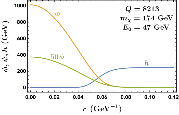 Figure 1
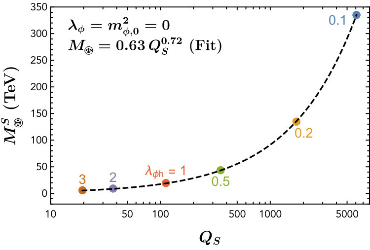 Figure 2
 Figure 3
 Figure 4
 Figure 5
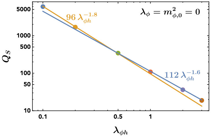 Figure 6
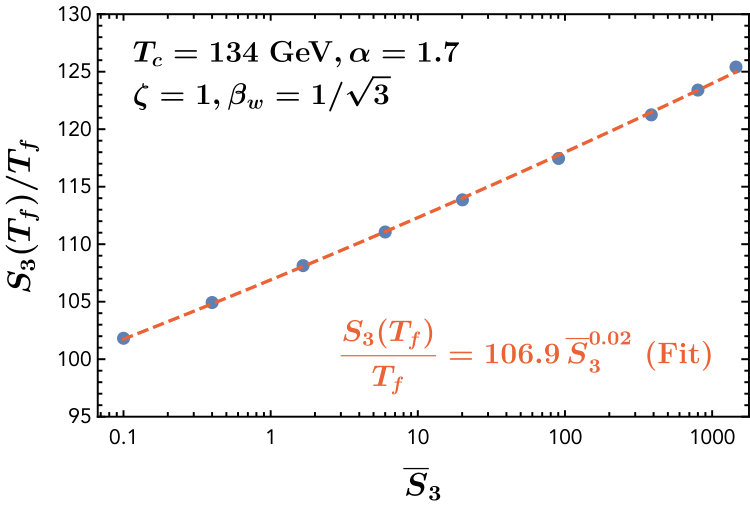 Figure 7
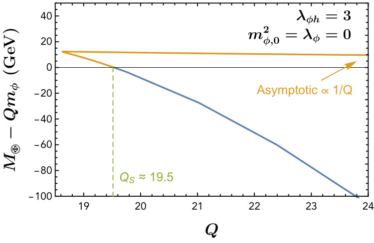 Figure 8
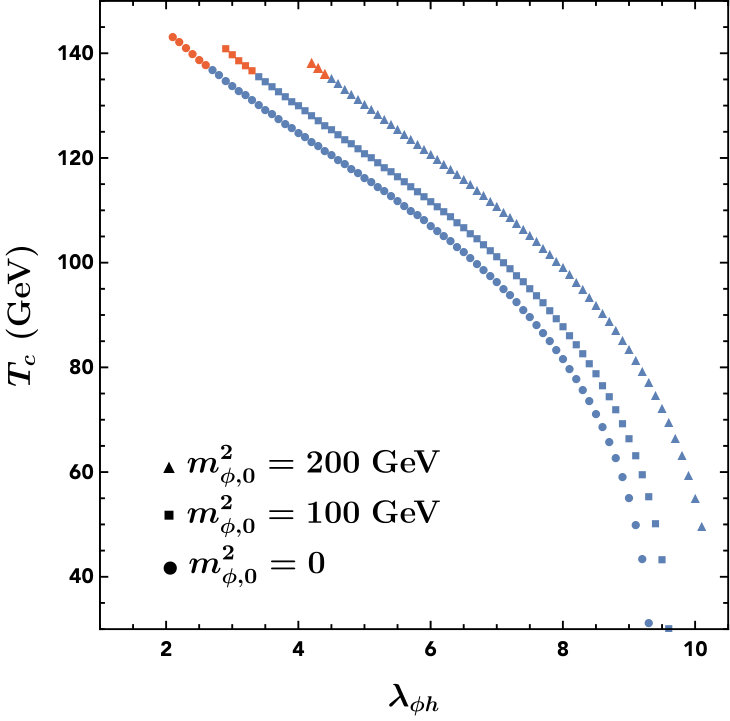 Figure 9
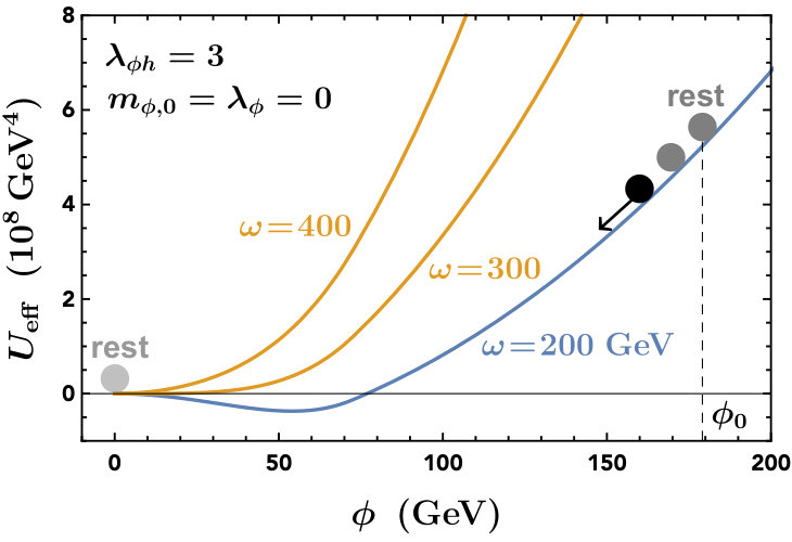 Figure 10
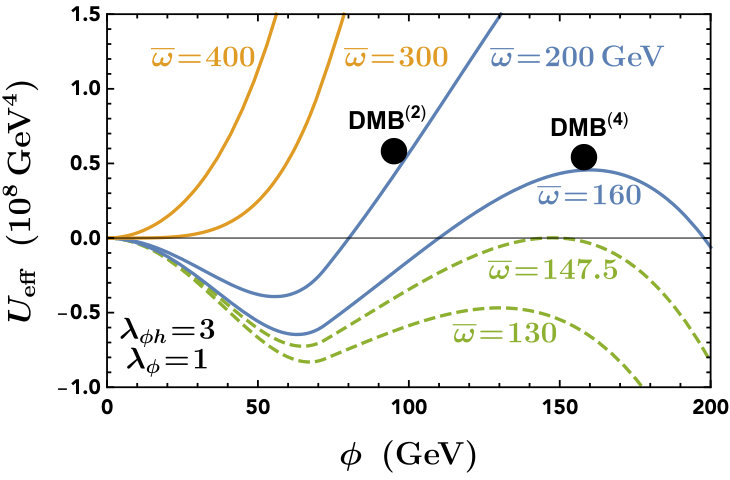 Figure 11
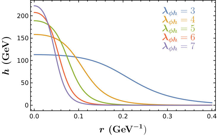 Figure 12
 Figure 13
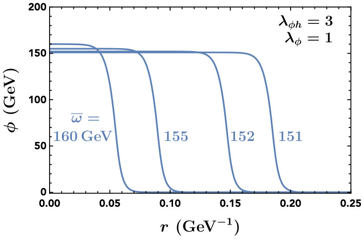 Figure 14
 Figure 15
 Figure 16
 Figure 17
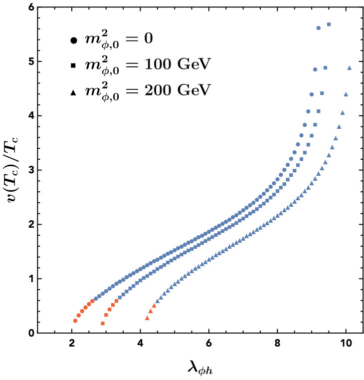 Figure 18
Peer Reviews
No public reviews on file for this paper yet. If you reviewed it on a platform where reviews are public (OpenReview, ICLR, NeurIPS, ICML), you can paste yours below so the community can read it here.
Videos
No videos yet. Explain this paper in a talk, walkthrough, or lecture? Add one.
\newfloatcommand
capbtabboxtable[][\FBwidth]
Electroweak Symmetric Dark Matter Balls
Eduardo Pontón, Yang Bai and Bithika Jain
(⋆*ICTP South American Institute for Fundamental Research & Instituto de Física Teórica
Universidade Estadual Paulista, São Paulo, Brazil
⋄Department of Physics, University of Wisconsin-Madison, Madison, WI 53706, USA
*)
Abstract
In the simple Higgs-portal dark matter model with a conserved dark matter number, we show that there exists a non-topological soliton state of dark matter. This state has smaller energy per dark matter number than a free particle state and has its interior in the electroweak symmetric vacuum. It could be produced in the early universe from first-order electroweak phase transition and contribute most of dark matter. This electroweak symmetric dark matter ball is a novel macroscopic dark matter candidate with an energy density of the electroweak scale and a mass of 1 gram or above. Because of its electroweak-symmetric interior, the dark matter ball has a large geometric scattering cross section off a nucleon or a nucleus. Dark matter and neutrino experiments with a large-size detector like Xenon1T, BOREXINO and JUNO have great potential to discover electroweak symmetric dark matter balls. We also discuss the formation of bound states of a dark matter ball and ordinary matter.
We are deeply saddened by the passing away of Eduardo Pontón (4 April 1971 – 13 June 2019). Eduardo has been an excellent mentor and collaborator. He has provided invaluable guidance for us from his passion and rigorous scientific attitude. We wish that he has a peaceful life in the other, maybe electroweak symmetric, world.
Contents
1 Introduction
Dark matter (DM) is one of the remaining mysteries in particle physics after the discovery of Higgs boson in 2012. After a few decades of searching for electroweak-sector-related dark matter particles with a mass around 100 GeV and with a null result [1], we have started to enlarge the scope of dark matter masses from both the theoretic model and the experimental search sides. For our visible sector, we have many interesting states of ordinary matter ranging from diluted gas to a dense neutron star. Analogously, it will not be surprising that there are many types of states for dark matter. Under certain circumstance, the majority of dark matter could be in a form of macroscopic state instead of free particle states. The well-known example is the primordial black hole dark matter [2], which has the Schwarzschild radius as its macroscopic size. Another established example the so-called “quark nugget” [3] with around nuclear energy density, which has the constituents of dark matter to be fermionic quarks and the geometrical size of – cm. In this paper, we will focus on another type of macroscopic dark matter with a bosonic constituent or “non-topological soliton” as named in the literature.
For a scalar field with non-linear interactions, it has long been pointed out that there exists a spacially-localized state that can be a solution to the scalar classical equation [4]. The existence and properties of the non-topological soliton as a field-theory object have been studied extensively by T. D. Lee [5] and S. R. Coleman [6] and their collaborators (see Ref. [7] for a review), while its primordial production from early universe physics has also been worked out in Refs. [8, 9, 10]. In supersymmetrical models, Q-balls (the soliton states and named by Coleman), built of squarks and sleptons have also been proposed as a potential dark matter candidate [11, 12, 13]. With a conserved global internal symmetry, the non-topological soliton is an extended object with the lowest value of the energy for a fixed conserved charge, and therefore is stable at quantum level. The non-topological soliton is simply different from topological solitons, which has a quantized charge related to the algebraic geometry. For instance, a nucleon can be regarded as a topological soliton state of pions or Skyrmion because of [14].
After some preparation of soliton basics, we want to point out the main observation of this paper: in the simple Higgs-portal complex scalar dark matter model, a non-topological soliton state exists for dark matter and could be the lowest energy state per dark matter number. For such a simple dark matter model, the dark matter could be in the macroscopic soliton state with a very large dark matter number, which we will refer as dark matter balls (DMBs). One possible mechanism to produce dark matter soliton states from early-universe dynamics could come from the first-order phase transition of electroweak (EW) symmetry, which can be naturally realized based on the quantum-corrected Higgs potential from the complex dark matter particle loop. Below the EW phase transition temperature, the EW symmetry-breaking bubbles grow and push the dark matter number to be in front of the bubble wall. After a few bubbles meet each other and coalesce, the dark matter number is enclosed in a small region and is still in the high-temperature EW-unbroken phase. Based on our later estimation and assuming some initial dark matter-antimatter asymmetry, we have found that the dark matter number is mainly stored in the soliton or DMB state instead of free dark matter particle state.
One interesting feature of DMBs based on the Higgs-portal dark matter model is the interplay between the Higgs potential and dark matter field strength. For a positive quartic interaction of the two fields, a large complex scalar dark matter field inside the DMB provides an effective positive mass for the Higgs field and prefers the Higgs field to sit at zero or a negligible value. So, the dark matter state could be a Electroweak Symmetric DM Ball (EWS-DMB) in sense that the electroweak symmetry is unbroken inside DMBs. This particular feature of DMB also means that the interaction of DMB with ordinary matter is relative large. From our later detailed calculations, we have found that the scattering cross section of DMBs off a nucleon or nucleus saturates to the geometrical cross section, when a DMB has a large radius.
Our observation could dramatically change the experimental search strategy for dark matter: instead of searching for the single-hit scattering event with a small recoil energy in a location deep underground, one could search for multi-hit scattering events at a location not necessarily underground. In consequence, neutrino-oriented experiments with a large size detector become suitable for this type of macroscopic dark matter. Or, searching for tracks in an ancient mineral like Mica may also discover this type of DMBs because of its very long, billion-year, exposure time. We will also discuss various search strategies for EWS-DMB.
The paper is organized as follows. We first work out the properties of soliton states with and without the dark matter bare mass and self-quartic interaction in Section 2. In Section 3, we study the early-universe productions of DMBs based on the first-order electroweak phase transition and obtain the characteristic charge, mass and radius for DMBs. We then calculate the scattering cross sections of DMBs with Standard Model (SM) particles in Section 4. The detection of DMBs in various experiments will be discussed in Section 5. We summarize our results in Section 6. Furthermore, we have also included four Appendixes: the calculation of the number of DMB nucleation sites in Appendix A, the calculation of the binding energy of bound states of EWS-DMBs and ordinary matter in Appendix B, the calculation of the bound states in a Higgs potential well in Appendix C and a simple example of scattering against a heavy object in Appendix D.
2 Soliton States in a Higgs-Portal Dark Matter Scenario
In the Higgs-portal dark matter scenario with a complex scalar particle ,111Although we will not do so here, one could consider the fermionic case. Due to the Pauli exclusion principle, it is qualitatively different from the bosonic example that is the focus of this work. the most general renormalizable Lagrangian preserving a symmetry is
[TABLE]
The symmetry ensures that the elementary quanta are stable, and therefore a DM candidate. This is one of the simplest extension of the SM to include dark matter. For reasons that will become clear in the following, we will focus on the region of parameter space with and , so that the physical mass squared is never negative, even in the absence of a vacuum expectation value (VEV) for . We will also take .222Furthermore, we restrict ourselves to the perturbative regime and . In this case, the global minimum of the tree-level potential breaks the EW symmetry spontaneously: with GeV, and . The quartic coupling is related to the Higgs boson mass GeV [15] by . After electroweak symmetry breaking (EWSB), the free particle mass is
[TABLE]
When the bare dark matter mass , the particle obtains all of its mass from EWSB and .
We are interested here in non-vacuum field configurations that are nevertheless stable due to the conservation of the charge associated with the global symmetry. In the theory given by Eq. (1), the existence and properties of such solutions were worked out in [5] (assuming and ), thus providing an example of a “non-topological soliton” (for a review, see [7]). We will briefly review how these solutions arise and their salient features. We start with the case and , to establish that such DM solitons exist even in this minimal case, which depends on a single free parameter, . This will also highlight the crucial role played by this coupling. In a second stage we will include the effects of the remaining two free parameters, and , which can affect the qualitative properties of the soliton solutions. We will describe the relevant features in Section 2.2.
The DM solitons are characterized by a non-vanishing charge
[TABLE]
which is obtained from the time-dependence , with real. We will focus on spherically symmetric solitons (that have the lowest energy) with and H^{T}=\big{(}0,h(r)/\sqrt{2}\big{)}, obeying the classical equations of motion
[TABLE]
and subject to the boundary conditions , and .
In order to develop an intuition it is useful to write down an approximate description by neglecting the Higgs derivatives in Eq. (5). The motivation is that often the Higgs profile is nearly vanishing inside the DM soliton and takes the (almost) constant value outside, approximating a step function. Thus, apart from the relatively small transition region, the neglect of the spatial derivatives can be justified a posteriori, thus permitting an effective description in terms of a single degree of freedom.333When the transition region is not small, the approximation can deviate by order one from the exact solution, but the qualitative features remain the same. We will also show numerical solutions that solve the full system of Eqs. (4) and (5). Eq. (5) then shows that one can have configurations obeying
[TABLE]
Inserting Eq. (8) into Eq. (4) one gets
[TABLE]
where the effective potential is obtained by using Eq. (8) in (minus) the potential terms of Eq. (1), but including the terms coming from the time derivatives:
[TABLE]
giving
[TABLE]
For later use, we reintroduced here the pure -dependent terms
[TABLE]
although for the time being we are setting them to zero. We then see that at large values, increases quadratically with . Importantly, the origin is unstable provided
[TABLE]
where we again wrote the dependence for later reference. As we will see, the small limit corresponds to large charge . Assuming Eq. (15), one can see that there is a solution that starting “at rest” (using an effective 1-particle mechanics in 1D language, with time evolution parametrized by ) at , rolls down the effective potential towards the hill at , loosing in the process energy due to the effective friction term in Eq. (9). It is clear that by adjusting , it is always possible to arrange for this motion to stop at . One can also see that since , one must have . At the saturation point of Eq. (15), the term in braces in evaluated at the matching point takes the positive value . Thus, for it is possible to find solutions fully contained in the region . Such solutions can have a non-negligible inside the core of the DM soliton, and typically require a more careful analysis that takes into account the derivatives that have been neglected in the effective description. However, when is very small, must be such that to satisfy . Translated into the behavior for this corresponds to situations with (nearly) vanishing inside the core of the DM soliton. We will therefore sometimes refer to such solutions as Electroweak Symmetric DM Balls (EWS-DMBs), or DMBs for short. The associated -profile typically resembles the step-like profile captured by the effective description.
We show in Fig. 1 the effective potential, , taking and , for several values of . The threshold value defined by the saturation of the inequality (15) is about GeV, and we show an example in its vicinity. Together with the GeV case, it gives rise to DM solitons with a sizable Higgs VEV inside the core. (As we will see, for GeV one obtains solutions displaying a core with a small Higgs VEV, i.e. an EWS-DMB.) Finally, the GeV case does not satisfy Eq. (15) and leads to oscillating solutions that tend slowly to zero as , and are therefore not localized. These do not belong in the class of solitonic solutions.
From the previous discussion, we also see that for DMB solutions one must have the scaling
[TABLE]
The size of the DMBs can be easily estimated as follows: setting in Eq. (4), as is appropriate inside the soliton, leads to
[TABLE]
This function has an infinite number of zeros, each of which corresponds to a solution. We will focus on the solution associated with the first zero, which has the lowest energy. Near this first zero, turns on leading quickly to the asymptotic value as (the excited solutions arise in a similar manner, but with additional nodes). The size of the transition, i.e. the thickness of the surface boundary separating the EW breaking and EW preserving phases is of order . We therefore see that the size of the lightest DMB, denoted by R_{\tiny\leavevmode\hbox to2.54pt{\vbox to2.54pt{\pgfpicture\makeatletter\hbox{\hskip 1.26836pt\lower-1.26836pt\hbox to0.0pt{\pgfsys@beginscope\pgfsys@invoke{ }\definecolor{pgfstrokecolor}{rgb}{0,0,0}\pgfsys@color@rgb@stroke{0}{0}{0}\pgfsys@invoke{ }\pgfsys@color@rgb@fill{0}{0}{0}\pgfsys@invoke{ }\pgfsys@setlinewidth{0.4pt}\pgfsys@invoke{ }\nullfont\hbox to0.0pt{\pgfsys@beginscope\pgfsys@invoke{ }{{}}\hbox{\hbox{{\pgfsys@beginscope\pgfsys@invoke{ }{{}{{{}}}{{}}{}{}{}{}{}{}{}{}{}{{}\pgfsys@moveto{1.06836pt}{0.0pt}\pgfsys@curveto{1.06836pt}{0.59004pt}{0.59004pt}{1.06836pt}{0.0pt}{1.06836pt}\pgfsys@curveto{-0.59004pt}{1.06836pt}{-1.06836pt}{0.59004pt}{-1.06836pt}{0.0pt}\pgfsys@curveto{-1.06836pt}{-0.59004pt}{-0.59004pt}{-1.06836pt}{0.0pt}{-1.06836pt}\pgfsys@curveto{0.59004pt}{-1.06836pt}{1.06836pt}{-0.59004pt}{1.06836pt}{0.0pt}\pgfsys@closepath\pgfsys@moveto{0.0pt}{0.0pt}\pgfsys@stroke\pgfsys@invoke{ } }{{{{}}\pgfsys@beginscope\pgfsys@invoke{ }\pgfsys@transformcm{1.0}{0.0}{0.0}{1.0}{-1.80556pt}{-1.20833pt}\pgfsys@invoke{ }\hbox{{\definecolor{pgfstrokecolor}{rgb}{0,0,0}\pgfsys@color@rgb@stroke{0}{0}{0}\pgfsys@invoke{ }\pgfsys@color@rgb@fill{0}{0}{0}\pgfsys@invoke{ }\hbox{{\raisebox{-0.5pt}[0.0pt]{\Phi}}} }}\pgfsys@invoke{\lxSVG@closescope }\pgfsys@endscope}}} \pgfsys@invoke{\lxSVG@closescope }\pgfsys@endscope}}} \pgfsys@invoke{\lxSVG@closescope }\pgfsys@endscope{{{}}}{}{}\hss}\pgfsys@discardpath\pgfsys@invoke{\lxSVG@closescope }\pgfsys@endscope\hss}}\lxSVG@closescope\endpgfpicture}}}, is about
[TABLE]
Inserting the approximate solution (17) in Eq. (3), together with Eq. (16), one finds
[TABLE]
As stated earlier, small maps into large . We also see that in this limit, we have the scaling
[TABLE]
With this qualitative understanding, let us now consider some examples of the full solutions to Eqs. (4) and (5).
2.1 Solutions to the Classical Equations of Motion
It is possible to obtain numerical solutions to the system (4) and (5) and the specified boundary conditions by the “shooting method”. This depends on two variables: and . The first derivatives vanish, which provides the four initial conditions to uniquely specify the solution. In practice, one starts at a small to avoid the singular point at the origin. One can then adjust and to obtain the solution that obeys and . In practice one takes to mean an large enough that the neglected part can be seen to be numerically close to the desired solution. This procedure can be followed for any fixed set of Lagrangian parameters, and fixed . For a given model, one is interested in scanning over , i.e. in obtaining soliton solutions of different charge .
We show in the left panel of Fig. 2 the (blue) and (orange) profiles for three different charges, in the model defined by and . The choice of is motivated by the mechanism of formation of such DM solitons, to be described later, but the features discussed in this section are similar for any of order one. The case (flatter, dashed profiles) corresponds to a choice of close to the threshold value defined by the saturation of the inequality (15). One can see that it is very close to the vacuum solution. There is a second solution with a similar charge with that displays a better defined core. As we will explain next, the former solution is unstable against decay into free elementary quanta, while the latter is a stable DM soliton. The third example has a larger charge , corresponding to a smaller GeV. It shows a clear core with a small Higgs VEV and a large value for . This DM soliton would fall in the category of EWS-DMBs defined above. Although the transition in the Higgs profile from zero to is comparable to the core, one can see that the profile is reasonably well described by the approximate solution (17) (for r\lesssim R_{\tiny\leavevmode\hbox to2.54pt{\vbox to2.54pt{\pgfpicture\makeatletter\hbox{\hskip 1.26836pt\lower-1.26836pt\hbox to0.0pt{\pgfsys@beginscope\pgfsys@invoke{ }\definecolor{pgfstrokecolor}{rgb}{0,0,0}\pgfsys@color@rgb@stroke{0}{0}{0}\pgfsys@invoke{ }\pgfsys@color@rgb@fill{0}{0}{0}\pgfsys@invoke{ }\pgfsys@setlinewidth{0.4pt}\pgfsys@invoke{ }\nullfont\hbox to0.0pt{\pgfsys@beginscope\pgfsys@invoke{ }{{}}\hbox{\hbox{{\pgfsys@beginscope\pgfsys@invoke{ }{{}{{{}}}{{}}{}{}{}{}{}{}{}{}{}{{}\pgfsys@moveto{1.06836pt}{0.0pt}\pgfsys@curveto{1.06836pt}{0.59004pt}{0.59004pt}{1.06836pt}{0.0pt}{1.06836pt}\pgfsys@curveto{-0.59004pt}{1.06836pt}{-1.06836pt}{0.59004pt}{-1.06836pt}{0.0pt}\pgfsys@curveto{-1.06836pt}{-0.59004pt}{-0.59004pt}{-1.06836pt}{0.0pt}{-1.06836pt}\pgfsys@curveto{0.59004pt}{-1.06836pt}{1.06836pt}{-0.59004pt}{1.06836pt}{0.0pt}\pgfsys@closepath\pgfsys@moveto{0.0pt}{0.0pt}\pgfsys@stroke\pgfsys@invoke{ } }{{{{}}\pgfsys@beginscope\pgfsys@invoke{ }\pgfsys@transformcm{1.0}{0.0}{0.0}{1.0}{-1.80556pt}{-1.20833pt}\pgfsys@invoke{ }\hbox{{\definecolor{pgfstrokecolor}{rgb}{0,0,0}\pgfsys@color@rgb@stroke{0}{0}{0}\pgfsys@invoke{ }\pgfsys@color@rgb@fill{0}{0}{0}\pgfsys@invoke{ }\hbox{{\raisebox{-0.5pt}[0.0pt]{\Phi}}} }}\pgfsys@invoke{\lxSVG@closescope }\pgfsys@endscope}}} \pgfsys@invoke{\lxSVG@closescope }\pgfsys@endscope}}} \pgfsys@invoke{\lxSVG@closescope }\pgfsys@endscope{{{}}}{}{}\hss}\pgfsys@discardpath\pgfsys@invoke{\lxSVG@closescope }\pgfsys@endscope\hss}}\lxSVG@closescope\endpgfpicture}}}). Indeed, for GeV, Eq. (18) gives R_{\tiny\leavevmode\hbox to2.54pt{\vbox to2.54pt{\pgfpicture\makeatletter\hbox{\hskip 1.26836pt\lower-1.26836pt\hbox to0.0pt{\pgfsys@beginscope\pgfsys@invoke{ }\definecolor{pgfstrokecolor}{rgb}{0,0,0}\pgfsys@color@rgb@stroke{0}{0}{0}\pgfsys@invoke{ }\pgfsys@color@rgb@fill{0}{0}{0}\pgfsys@invoke{ }\pgfsys@setlinewidth{0.4pt}\pgfsys@invoke{ }\nullfont\hbox to0.0pt{\pgfsys@beginscope\pgfsys@invoke{ }{{}}\hbox{\hbox{{\pgfsys@beginscope\pgfsys@invoke{ }{{}{{{}}}{{}}{}{}{}{}{}{}{}{}{}{{}\pgfsys@moveto{1.06836pt}{0.0pt}\pgfsys@curveto{1.06836pt}{0.59004pt}{0.59004pt}{1.06836pt}{0.0pt}{1.06836pt}\pgfsys@curveto{-0.59004pt}{1.06836pt}{-1.06836pt}{0.59004pt}{-1.06836pt}{0.0pt}\pgfsys@curveto{-1.06836pt}{-0.59004pt}{-0.59004pt}{-1.06836pt}{0.0pt}{-1.06836pt}\pgfsys@curveto{0.59004pt}{-1.06836pt}{1.06836pt}{-0.59004pt}{1.06836pt}{0.0pt}\pgfsys@closepath\pgfsys@moveto{0.0pt}{0.0pt}\pgfsys@stroke\pgfsys@invoke{ } }{{{{}}\pgfsys@beginscope\pgfsys@invoke{ }\pgfsys@transformcm{1.0}{0.0}{0.0}{1.0}{-1.80556pt}{-1.20833pt}\pgfsys@invoke{ }\hbox{{\definecolor{pgfstrokecolor}{rgb}{0,0,0}\pgfsys@color@rgb@stroke{0}{0}{0}\pgfsys@invoke{ }\pgfsys@color@rgb@fill{0}{0}{0}\pgfsys@invoke{ }\hbox{{\raisebox{-0.5pt}[0.0pt]{\Phi}}} }}\pgfsys@invoke{\lxSVG@closescope }\pgfsys@endscope}}} \pgfsys@invoke{\lxSVG@closescope }\pgfsys@endscope}}} \pgfsys@invoke{\lxSVG@closescope }\pgfsys@endscope{{{}}}{}{}\hss}\pgfsys@discardpath\pgfsys@invoke{\lxSVG@closescope }\pgfsys@endscope\hss}}\lxSVG@closescope\endpgfpicture}}}\approx 0.03\leavevmode\nobreak\ {\rm GeV}^{-1}, in good agreement with what is seen in the figure. Obtaining full numerical solutions with larger cores is challenging, as the solutions are sensitive to an exponentially small . Such solutions can nevertheless be easily obtained in the framework of the effective description. We will also use the effective description to discuss the effects of the two additional parameters, and .
Before turning to the general case, we consider the mass of the DM soliton. In the mean field approximation we are using, this can be obtained by computing the classical energy of the configuration:
[TABLE]
where is the SM Higgs potential and was defined in Eq. (14). Here, and are derivatives with respect to . Note that localized field configurations cannot have a well-defined energy: although the mean energy in the rest frame is given by M_{\tiny\leavevmode\hbox to2.54pt{\vbox to2.54pt{\pgfpicture\makeatletter\hbox{\hskip 1.26836pt\lower-1.26836pt\hbox to0.0pt{\pgfsys@beginscope\pgfsys@invoke{ }\definecolor{pgfstrokecolor}{rgb}{0,0,0}\pgfsys@color@rgb@stroke{0}{0}{0}\pgfsys@invoke{ }\pgfsys@color@rgb@fill{0}{0}{0}\pgfsys@invoke{ }\pgfsys@setlinewidth{0.4pt}\pgfsys@invoke{ }\nullfont\hbox to0.0pt{\pgfsys@beginscope\pgfsys@invoke{ }{{}}\hbox{\hbox{{\pgfsys@beginscope\pgfsys@invoke{ }{{}{{{}}}{{}}{}{}{}{}{}{}{}{}{}{{}\pgfsys@moveto{1.06836pt}{0.0pt}\pgfsys@curveto{1.06836pt}{0.59004pt}{0.59004pt}{1.06836pt}{0.0pt}{1.06836pt}\pgfsys@curveto{-0.59004pt}{1.06836pt}{-1.06836pt}{0.59004pt}{-1.06836pt}{0.0pt}\pgfsys@curveto{-1.06836pt}{-0.59004pt}{-0.59004pt}{-1.06836pt}{0.0pt}{-1.06836pt}\pgfsys@curveto{0.59004pt}{-1.06836pt}{1.06836pt}{-0.59004pt}{1.06836pt}{0.0pt}\pgfsys@closepath\pgfsys@moveto{0.0pt}{0.0pt}\pgfsys@stroke\pgfsys@invoke{ } }{{{{}}\pgfsys@beginscope\pgfsys@invoke{ }\pgfsys@transformcm{1.0}{0.0}{0.0}{1.0}{-1.80556pt}{-1.20833pt}\pgfsys@invoke{ }\hbox{{\definecolor{pgfstrokecolor}{rgb}{0,0,0}\pgfsys@color@rgb@stroke{0}{0}{0}\pgfsys@invoke{ }\pgfsys@color@rgb@fill{0}{0}{0}\pgfsys@invoke{ }\hbox{{\raisebox{-0.5pt}[0.0pt]{\Phi}}} }}\pgfsys@invoke{\lxSVG@closescope }\pgfsys@endscope}}} \pgfsys@invoke{\lxSVG@closescope }\pgfsys@endscope}}} \pgfsys@invoke{\lxSVG@closescope }\pgfsys@endscope{{{}}}{}{}\hss}\pgfsys@discardpath\pgfsys@invoke{\lxSVG@closescope }\pgfsys@endscope\hss}}\lxSVG@closescope\endpgfpicture}}}, there are quantum mechanical fluctuations in the 3-momentum. Such effects can be taken into account by a proper separation between the collective center of mass coordinates and the vibrational modes. This can be achieved by defining appropriate coherent states followed by a projection onto zero-momentum eigenstates [16]. We will ignore such corrections and use M_{\tiny\leavevmode\hbox to2.54pt{\vbox to2.54pt{\pgfpicture\makeatletter\hbox{\hskip 1.26836pt\lower-1.26836pt\hbox to0.0pt{\pgfsys@beginscope\pgfsys@invoke{ }\definecolor{pgfstrokecolor}{rgb}{0,0,0}\pgfsys@color@rgb@stroke{0}{0}{0}\pgfsys@invoke{ }\pgfsys@color@rgb@fill{0}{0}{0}\pgfsys@invoke{ }\pgfsys@setlinewidth{0.4pt}\pgfsys@invoke{ }\nullfont\hbox to0.0pt{\pgfsys@beginscope\pgfsys@invoke{ }{{}}\hbox{\hbox{{\pgfsys@beginscope\pgfsys@invoke{ }{{}{{{}}}{{}}{}{}{}{}{}{}{}{}{}{{}\pgfsys@moveto{1.06836pt}{0.0pt}\pgfsys@curveto{1.06836pt}{0.59004pt}{0.59004pt}{1.06836pt}{0.0pt}{1.06836pt}\pgfsys@curveto{-0.59004pt}{1.06836pt}{-1.06836pt}{0.59004pt}{-1.06836pt}{0.0pt}\pgfsys@curveto{-1.06836pt}{-0.59004pt}{-0.59004pt}{-1.06836pt}{0.0pt}{-1.06836pt}\pgfsys@curveto{0.59004pt}{-1.06836pt}{1.06836pt}{-0.59004pt}{1.06836pt}{0.0pt}\pgfsys@closepath\pgfsys@moveto{0.0pt}{0.0pt}\pgfsys@stroke\pgfsys@invoke{ } }{{{{}}\pgfsys@beginscope\pgfsys@invoke{ }\pgfsys@transformcm{1.0}{0.0}{0.0}{1.0}{-1.80556pt}{-1.20833pt}\pgfsys@invoke{ }\hbox{{\definecolor{pgfstrokecolor}{rgb}{0,0,0}\pgfsys@color@rgb@stroke{0}{0}{0}\pgfsys@invoke{ }\pgfsys@color@rgb@fill{0}{0}{0}\pgfsys@invoke{ }\hbox{{\raisebox{-0.5pt}[0.0pt]{\Phi}}} }}\pgfsys@invoke{\lxSVG@closescope }\pgfsys@endscope}}} \pgfsys@invoke{\lxSVG@closescope }\pgfsys@endscope}}} \pgfsys@invoke{\lxSVG@closescope }\pgfsys@endscope{{{}}}{}{}\hss}\pgfsys@discardpath\pgfsys@invoke{\lxSVG@closescope }\pgfsys@endscope\hss}}\lxSVG@closescope\endpgfpicture}}} above as a proxy for the soliton mass, since the above precision is sufficient for our purposes.
We show in the right panel of Fig. 2 the mass of the lightest DM soliton as a function of .444We show here the low region of a scan over , obtained by solving the EOM numerically, as described above. However, for the (almost) horizontal (orange) part of the curve we use instead the first order approximation (for ) derived in [5]: M_{\tiny\leavevmode\hbox to2.54pt{\vbox to2.54pt{\pgfpicture\makeatletter\hbox{\hskip 1.26836pt\lower-1.26836pt\hbox to0.0pt{\pgfsys@beginscope\pgfsys@invoke{ }\definecolor{pgfstrokecolor}{rgb}{0,0,0}\pgfsys@color@rgb@stroke{0}{0}{0}\pgfsys@invoke{ }\pgfsys@color@rgb@fill{0}{0}{0}\pgfsys@invoke{ }\pgfsys@setlinewidth{0.4pt}\pgfsys@invoke{ }\nullfont\hbox to0.0pt{\pgfsys@beginscope\pgfsys@invoke{ }{{}}\hbox{\hbox{{\pgfsys@beginscope\pgfsys@invoke{ }{{}{{{}}}{{}}{}{}{}{}{}{}{}{}{}{{}\pgfsys@moveto{1.06836pt}{0.0pt}\pgfsys@curveto{1.06836pt}{0.59004pt}{0.59004pt}{1.06836pt}{0.0pt}{1.06836pt}\pgfsys@curveto{-0.59004pt}{1.06836pt}{-1.06836pt}{0.59004pt}{-1.06836pt}{0.0pt}\pgfsys@curveto{-1.06836pt}{-0.59004pt}{-0.59004pt}{-1.06836pt}{0.0pt}{-1.06836pt}\pgfsys@curveto{0.59004pt}{-1.06836pt}{1.06836pt}{-0.59004pt}{1.06836pt}{0.0pt}\pgfsys@closepath\pgfsys@moveto{0.0pt}{0.0pt}\pgfsys@stroke\pgfsys@invoke{ } }{{{{}}\pgfsys@beginscope\pgfsys@invoke{ }\pgfsys@transformcm{1.0}{0.0}{0.0}{1.0}{-1.80556pt}{-1.20833pt}\pgfsys@invoke{ }\hbox{{\definecolor{pgfstrokecolor}{rgb}{0,0,0}\pgfsys@color@rgb@stroke{0}{0}{0}\pgfsys@invoke{ }\pgfsys@color@rgb@fill{0}{0}{0}\pgfsys@invoke{ }\hbox{{\raisebox{-0.5pt}[0.0pt]{\Phi}}} }}\pgfsys@invoke{\lxSVG@closescope }\pgfsys@endscope}}} \pgfsys@invoke{\lxSVG@closescope }\pgfsys@endscope}}} \pgfsys@invoke{\lxSVG@closescope }\pgfsys@endscope{{{}}}{}{}\hss}\pgfsys@discardpath\pgfsys@invoke{\lxSVG@closescope }\pgfsys@endscope\hss}}\lxSVG@closescope\endpgfpicture}}}-Qm_{\phi}=(2\pi^{2}M_{2}^{2}m_{h}^{8})/(\lambda_{h}^{2}m_{\phi}^{7}Q)+{\cal O}(Q^{-3}) where the moment is calculable and gives . The reason is that in this region the excited states are split by small energy differences (that tend to zero as on this branch), and it is difficult to isolate the ground state numerically.
One can distinguish two branches as one increases from small values up to where the DM soliton solutions cease to exist. The charge decreases monotonically down to a minimum value ( in the figure), then increases rapidly again and diverges as . It can be shown that all such DM soliton solutions are stable against small classical fluctuations [5]. It is, however, important to compare the DM soliton mass against the energy of free elementary quanta. We plot the difference M_{\tiny\leavevmode\hbox to2.54pt{\vbox to2.54pt{\pgfpicture\makeatletter\hbox{\hskip 1.26836pt\lower-1.26836pt\hbox to0.0pt{\pgfsys@beginscope\pgfsys@invoke{ }\definecolor{pgfstrokecolor}{rgb}{0,0,0}\pgfsys@color@rgb@stroke{0}{0}{0}\pgfsys@invoke{ }\pgfsys@color@rgb@fill{0}{0}{0}\pgfsys@invoke{ }\pgfsys@setlinewidth{0.4pt}\pgfsys@invoke{ }\nullfont\hbox to0.0pt{\pgfsys@beginscope\pgfsys@invoke{ }{{}}\hbox{\hbox{{\pgfsys@beginscope\pgfsys@invoke{ }{{}{{{}}}{{}}{}{}{}{}{}{}{}{}{}{{}\pgfsys@moveto{1.06836pt}{0.0pt}\pgfsys@curveto{1.06836pt}{0.59004pt}{0.59004pt}{1.06836pt}{0.0pt}{1.06836pt}\pgfsys@curveto{-0.59004pt}{1.06836pt}{-1.06836pt}{0.59004pt}{-1.06836pt}{0.0pt}\pgfsys@curveto{-1.06836pt}{-0.59004pt}{-0.59004pt}{-1.06836pt}{0.0pt}{-1.06836pt}\pgfsys@curveto{0.59004pt}{-1.06836pt}{1.06836pt}{-0.59004pt}{1.06836pt}{0.0pt}\pgfsys@closepath\pgfsys@moveto{0.0pt}{0.0pt}\pgfsys@stroke\pgfsys@invoke{ } }{{{{}}\pgfsys@beginscope\pgfsys@invoke{ }\pgfsys@transformcm{1.0}{0.0}{0.0}{1.0}{-1.80556pt}{-1.20833pt}\pgfsys@invoke{ }\hbox{{\definecolor{pgfstrokecolor}{rgb}{0,0,0}\pgfsys@color@rgb@stroke{0}{0}{0}\pgfsys@invoke{ }\pgfsys@color@rgb@fill{0}{0}{0}\pgfsys@invoke{ }\hbox{{\raisebox{-0.5pt}[0.0pt]{\Phi}}} }}\pgfsys@invoke{\lxSVG@closescope }\pgfsys@endscope}}} \pgfsys@invoke{\lxSVG@closescope }\pgfsys@endscope}}} \pgfsys@invoke{\lxSVG@closescope }\pgfsys@endscope{{{}}}{}{}\hss}\pgfsys@discardpath\pgfsys@invoke{\lxSVG@closescope }\pgfsys@endscope\hss}}\lxSVG@closescope\endpgfpicture}}}-Qm_{\phi}, which shows that there are two branches to be distinguished. The first branch (orange) is unstable against quantum mechanical decay into free particle states. The second branch (blue) is forbidden from decaying by a combination of energetic considerations and the conservation of the charge. In fact, they correspond to stable quantum mechanical states. This defines a that separates the two types of solutions. For the model parameters used in the figure, one finds (corresponding to GeV). Thus, the profiles in the left panel of the figure correspond to an unstable soliton, while the and cases correspond to stable DM solitons.
In order to establish the scaling of M_{\tiny\leavevmode\hbox to2.54pt{\vbox to2.54pt{\pgfpicture\makeatletter\hbox{\hskip 1.26836pt\lower-1.26836pt\hbox to0.0pt{\pgfsys@beginscope\pgfsys@invoke{ }\definecolor{pgfstrokecolor}{rgb}{0,0,0}\pgfsys@color@rgb@stroke{0}{0}{0}\pgfsys@invoke{ }\pgfsys@color@rgb@fill{0}{0}{0}\pgfsys@invoke{ }\pgfsys@setlinewidth{0.4pt}\pgfsys@invoke{ }\nullfont\hbox to0.0pt{\pgfsys@beginscope\pgfsys@invoke{ }{{}}\hbox{\hbox{{\pgfsys@beginscope\pgfsys@invoke{ }{{}{{{}}}{{}}{}{}{}{}{}{}{}{}{}{{}\pgfsys@moveto{1.06836pt}{0.0pt}\pgfsys@curveto{1.06836pt}{0.59004pt}{0.59004pt}{1.06836pt}{0.0pt}{1.06836pt}\pgfsys@curveto{-0.59004pt}{1.06836pt}{-1.06836pt}{0.59004pt}{-1.06836pt}{0.0pt}\pgfsys@curveto{-1.06836pt}{-0.59004pt}{-0.59004pt}{-1.06836pt}{0.0pt}{-1.06836pt}\pgfsys@curveto{0.59004pt}{-1.06836pt}{1.06836pt}{-0.59004pt}{1.06836pt}{0.0pt}\pgfsys@closepath\pgfsys@moveto{0.0pt}{0.0pt}\pgfsys@stroke\pgfsys@invoke{ } }{{{{}}\pgfsys@beginscope\pgfsys@invoke{ }\pgfsys@transformcm{1.0}{0.0}{0.0}{1.0}{-1.80556pt}{-1.20833pt}\pgfsys@invoke{ }\hbox{{\definecolor{pgfstrokecolor}{rgb}{0,0,0}\pgfsys@color@rgb@stroke{0}{0}{0}\pgfsys@invoke{ }\pgfsys@color@rgb@fill{0}{0}{0}\pgfsys@invoke{ }\hbox{{\raisebox{-0.5pt}[0.0pt]{\Phi}}} }}\pgfsys@invoke{\lxSVG@closescope }\pgfsys@endscope}}} \pgfsys@invoke{\lxSVG@closescope }\pgfsys@endscope}}} \pgfsys@invoke{\lxSVG@closescope }\pgfsys@endscope{{{}}}{}{}\hss}\pgfsys@discardpath\pgfsys@invoke{\lxSVG@closescope }\pgfsys@endscope\hss}}\lxSVG@closescope\endpgfpicture}}} with , let us focus on DMBs by assuming that the field vanishes inside the core. Then is given by Eq. (17) for r<R_{\tiny\leavevmode\hbox to2.54pt{\vbox to2.54pt{\pgfpicture\makeatletter\hbox{\hskip 1.26836pt\lower-1.26836pt\hbox to0.0pt{\pgfsys@beginscope\pgfsys@invoke{ }\definecolor{pgfstrokecolor}{rgb}{0,0,0}\pgfsys@color@rgb@stroke{0}{0}{0}\pgfsys@invoke{ }\pgfsys@color@rgb@fill{0}{0}{0}\pgfsys@invoke{ }\pgfsys@setlinewidth{0.4pt}\pgfsys@invoke{ }\nullfont\hbox to0.0pt{\pgfsys@beginscope\pgfsys@invoke{ }{{}}\hbox{\hbox{{\pgfsys@beginscope\pgfsys@invoke{ }{{}{{{}}}{{}}{}{}{}{}{}{}{}{}{}{{}\pgfsys@moveto{1.06836pt}{0.0pt}\pgfsys@curveto{1.06836pt}{0.59004pt}{0.59004pt}{1.06836pt}{0.0pt}{1.06836pt}\pgfsys@curveto{-0.59004pt}{1.06836pt}{-1.06836pt}{0.59004pt}{-1.06836pt}{0.0pt}\pgfsys@curveto{-1.06836pt}{-0.59004pt}{-0.59004pt}{-1.06836pt}{0.0pt}{-1.06836pt}\pgfsys@curveto{0.59004pt}{-1.06836pt}{1.06836pt}{-0.59004pt}{1.06836pt}{0.0pt}\pgfsys@closepath\pgfsys@moveto{0.0pt}{0.0pt}\pgfsys@stroke\pgfsys@invoke{ } }{{{{}}\pgfsys@beginscope\pgfsys@invoke{ }\pgfsys@transformcm{1.0}{0.0}{0.0}{1.0}{-1.80556pt}{-1.20833pt}\pgfsys@invoke{ }\hbox{{\definecolor{pgfstrokecolor}{rgb}{0,0,0}\pgfsys@color@rgb@stroke{0}{0}{0}\pgfsys@invoke{ }\pgfsys@color@rgb@fill{0}{0}{0}\pgfsys@invoke{ }\hbox{{\raisebox{-0.5pt}[0.0pt]{\Phi}}} }}\pgfsys@invoke{\lxSVG@closescope }\pgfsys@endscope}}} \pgfsys@invoke{\lxSVG@closescope }\pgfsys@endscope}}} \pgfsys@invoke{\lxSVG@closescope }\pgfsys@endscope{{{}}}{}{}\hss}\pgfsys@discardpath\pgfsys@invoke{\lxSVG@closescope }\pgfsys@endscope\hss}}\lxSVG@closescope\endpgfpicture}}}\approx\pi/\omega (and zero for r>R_{\tiny\leavevmode\hbox to2.54pt{\vbox to2.54pt{\pgfpicture\makeatletter\hbox{\hskip 1.26836pt\lower-1.26836pt\hbox to0.0pt{\pgfsys@beginscope\pgfsys@invoke{ }\definecolor{pgfstrokecolor}{rgb}{0,0,0}\pgfsys@color@rgb@stroke{0}{0}{0}\pgfsys@invoke{ }\pgfsys@color@rgb@fill{0}{0}{0}\pgfsys@invoke{ }\pgfsys@setlinewidth{0.4pt}\pgfsys@invoke{ }\nullfont\hbox to0.0pt{\pgfsys@beginscope\pgfsys@invoke{ }{{}}\hbox{\hbox{{\pgfsys@beginscope\pgfsys@invoke{ }{{}{{{}}}{{}}{}{}{}{}{}{}{}{}{}{{}\pgfsys@moveto{1.06836pt}{0.0pt}\pgfsys@curveto{1.06836pt}{0.59004pt}{0.59004pt}{1.06836pt}{0.0pt}{1.06836pt}\pgfsys@curveto{-0.59004pt}{1.06836pt}{-1.06836pt}{0.59004pt}{-1.06836pt}{0.0pt}\pgfsys@curveto{-1.06836pt}{-0.59004pt}{-0.59004pt}{-1.06836pt}{0.0pt}{-1.06836pt}\pgfsys@curveto{0.59004pt}{-1.06836pt}{1.06836pt}{-0.59004pt}{1.06836pt}{0.0pt}\pgfsys@closepath\pgfsys@moveto{0.0pt}{0.0pt}\pgfsys@stroke\pgfsys@invoke{ } }{{{{}}\pgfsys@beginscope\pgfsys@invoke{ }\pgfsys@transformcm{1.0}{0.0}{0.0}{1.0}{-1.80556pt}{-1.20833pt}\pgfsys@invoke{ }\hbox{{\definecolor{pgfstrokecolor}{rgb}{0,0,0}\pgfsys@color@rgb@stroke{0}{0}{0}\pgfsys@invoke{ }\pgfsys@color@rgb@fill{0}{0}{0}\pgfsys@invoke{ }\hbox{{\raisebox{-0.5pt}[0.0pt]{\Phi}}} }}\pgfsys@invoke{\lxSVG@closescope }\pgfsys@endscope}}} \pgfsys@invoke{\lxSVG@closescope }\pgfsys@endscope}}} \pgfsys@invoke{\lxSVG@closescope }\pgfsys@endscope{{{}}}{}{}\hss}\pgfsys@discardpath\pgfsys@invoke{\lxSVG@closescope }\pgfsys@endscope\hss}}\lxSVG@closescope\endpgfpicture}}}). Neglecting the surface tension contributions from (i.e. setting everywhere), one has from Eq. (21):
[TABLE]
where we exchanged for using Eq. (19). We are interested in the lowest energy solution for fixed . Minimizing against the dynamical variable , we find that the minimum is at
[TABLE]
Thus, together with the results of the previous section, we have that for DMBs in the case that , the following scaling laws between the charge, the size, and the mass of the DMB apply 555We will see in the next section that by itself does not change these scaling relations.
[TABLE]
These scaling laws hold for DM solitons with a large . In the low region displayed in the right panel of Fig. 2 somewhat different relations are obeyed, that can only be found by a more detailed numerical analysis.
We focus on the stability point associated with the charge that delimits the stable/unstable soliton configurations. In the left panel of Fig. 3 we show the corresponding DM soliton mass, M_{\tiny\leavevmode\hbox to2.54pt{\vbox to2.54pt{\pgfpicture\makeatletter\hbox{\hskip 1.26836pt\lower-1.26836pt\hbox to0.0pt{\pgfsys@beginscope\pgfsys@invoke{ }\definecolor{pgfstrokecolor}{rgb}{0,0,0}\pgfsys@color@rgb@stroke{0}{0}{0}\pgfsys@invoke{ }\pgfsys@color@rgb@fill{0}{0}{0}\pgfsys@invoke{ }\pgfsys@setlinewidth{0.4pt}\pgfsys@invoke{ }\nullfont\hbox to0.0pt{\pgfsys@beginscope\pgfsys@invoke{ }{{}}\hbox{\hbox{{\pgfsys@beginscope\pgfsys@invoke{ }{{}{{{}}}{{}}{}{}{}{}{}{}{}{}{}{{}\pgfsys@moveto{1.06836pt}{0.0pt}\pgfsys@curveto{1.06836pt}{0.59004pt}{0.59004pt}{1.06836pt}{0.0pt}{1.06836pt}\pgfsys@curveto{-0.59004pt}{1.06836pt}{-1.06836pt}{0.59004pt}{-1.06836pt}{0.0pt}\pgfsys@curveto{-1.06836pt}{-0.59004pt}{-0.59004pt}{-1.06836pt}{0.0pt}{-1.06836pt}\pgfsys@curveto{0.59004pt}{-1.06836pt}{1.06836pt}{-0.59004pt}{1.06836pt}{0.0pt}\pgfsys@closepath\pgfsys@moveto{0.0pt}{0.0pt}\pgfsys@stroke\pgfsys@invoke{ } }{{{{}}\pgfsys@beginscope\pgfsys@invoke{ }\pgfsys@transformcm{1.0}{0.0}{0.0}{1.0}{-1.80556pt}{-1.20833pt}\pgfsys@invoke{ }\hbox{{\definecolor{pgfstrokecolor}{rgb}{0,0,0}\pgfsys@color@rgb@stroke{0}{0}{0}\pgfsys@invoke{ }\pgfsys@color@rgb@fill{0}{0}{0}\pgfsys@invoke{ }\hbox{{\raisebox{-0.5pt}[0.0pt]{\Phi}}} }}\pgfsys@invoke{\lxSVG@closescope }\pgfsys@endscope}}} \pgfsys@invoke{\lxSVG@closescope }\pgfsys@endscope}}} \pgfsys@invoke{\lxSVG@closescope }\pgfsys@endscope{{{}}}{}{}\hss}\pgfsys@discardpath\pgfsys@invoke{\lxSVG@closescope }\pgfsys@endscope\hss}}\lxSVG@closescope\endpgfpicture}}}^{S}, as a function of , as we vary in the range . The simulated models are well fitted by 666If one uses Eq. (23) to determine , even though it is not meant to hold for the lowest charges corresponding to DM solitons that are not DMBs, one can estimate . This gives a reasonable order of magnitude estimate for , working better for larger .
[TABLE]
This is a parametric relation across models as we vary . The parametric dependence for is shown in the right panel of Fig. 3, and can be reproduced by a broken power law in this range, as shown in the figure. From the information in both panels one can get M_{\tiny\leavevmode\hbox to2.54pt{\vbox to2.54pt{\pgfpicture\makeatletter\hbox{\hskip 1.26836pt\lower-1.26836pt\hbox to0.0pt{\pgfsys@beginscope\pgfsys@invoke{ }\definecolor{pgfstrokecolor}{rgb}{0,0,0}\pgfsys@color@rgb@stroke{0}{0}{0}\pgfsys@invoke{ }\pgfsys@color@rgb@fill{0}{0}{0}\pgfsys@invoke{ }\pgfsys@setlinewidth{0.4pt}\pgfsys@invoke{ }\nullfont\hbox to0.0pt{\pgfsys@beginscope\pgfsys@invoke{ }{{}}\hbox{\hbox{{\pgfsys@beginscope\pgfsys@invoke{ }{{}{{{}}}{{}}{}{}{}{}{}{}{}{}{}{{}\pgfsys@moveto{1.06836pt}{0.0pt}\pgfsys@curveto{1.06836pt}{0.59004pt}{0.59004pt}{1.06836pt}{0.0pt}{1.06836pt}\pgfsys@curveto{-0.59004pt}{1.06836pt}{-1.06836pt}{0.59004pt}{-1.06836pt}{0.0pt}\pgfsys@curveto{-1.06836pt}{-0.59004pt}{-0.59004pt}{-1.06836pt}{0.0pt}{-1.06836pt}\pgfsys@curveto{0.59004pt}{-1.06836pt}{1.06836pt}{-0.59004pt}{1.06836pt}{0.0pt}\pgfsys@closepath\pgfsys@moveto{0.0pt}{0.0pt}\pgfsys@stroke\pgfsys@invoke{ } }{{{{}}\pgfsys@beginscope\pgfsys@invoke{ }\pgfsys@transformcm{1.0}{0.0}{0.0}{1.0}{-1.80556pt}{-1.20833pt}\pgfsys@invoke{ }\hbox{{\definecolor{pgfstrokecolor}{rgb}{0,0,0}\pgfsys@color@rgb@stroke{0}{0}{0}\pgfsys@invoke{ }\pgfsys@color@rgb@fill{0}{0}{0}\pgfsys@invoke{ }\hbox{{\raisebox{-0.5pt}[0.0pt]{\Phi}}} }}\pgfsys@invoke{\lxSVG@closescope }\pgfsys@endscope}}} \pgfsys@invoke{\lxSVG@closescope }\pgfsys@endscope}}} \pgfsys@invoke{\lxSVG@closescope }\pgfsys@endscope{{{}}}{}{}\hss}\pgfsys@discardpath\pgfsys@invoke{\lxSVG@closescope }\pgfsys@endscope\hss}}\lxSVG@closescope\endpgfpicture}}}^{S}(\lambda_{\phi h}). One can similarly consider the radius for such a minimum charge DM soliton, which is well described by
[TABLE]
Thus, the typical radii for such charges are of order , while the masses are in the tens of TeV and above region. These scales arise from the weak scale due to charge enhancements, qualitatively similar to the scaling laws discussed above, but not as simple. Based on these plots we can estimate the energy density associated with the DM soliton configuration to be of order
[TABLE]
To the extent that the scaling laws given in Eq. (24) connect the low and high cases, we expect the same estimate to hold for very large DMBs.
2.2 Effects of the Dark Matter Bare Mass and Self-Quartic Interaction
We now comment on the effects of the remaining two parameters of the model, and . Within the context of the effective potential description defined in Eq. (13), one can see that
The bare mass can be easily included by defining an effective in the effective potential and associated EOM. One must only remember that when computing observables such as the mass of the DM soliton via Eq. (21), it is the orthogonal combination that appears. Similarly, the charge is proportional to , and the combination enters only through . With the solutions for the case at hand this can be easily taken into account. 2. 2.
The quartic self-interaction has a more significant effect: it changes the large behavior of the effective potential from the quadratic one used in the previous section, turning it down to reach an asymptotic behavior (for ) (see the left panel of Fig. 4). This creates a maximum in the potential at some . The soliton solutions must therefore satisfy , since for the solutions would run down the hill in the wrong direction and not be bounded. This is the scenario considered for -balls in Ref. [6], and we know that stable solitonic configurations exist in this case.
The first point could mean that even for ultraheavy elementary particles that receive only a small contribution to their mass from EWSB, it could be possible to have solitonic configurations related to the weak scale, i.e. sustaining an EW symmetric “vacuum” in a finite region of space, inside the normal EW breaking vacuum.
Let us now describe some of the consequences of the quartic coupling , assuming for simplicity that we are interested in DM solitons with a large charge , such that they fall in the class of EWS-DMBs. In this case, the maximum of the effective potential described in point 2 above lies in the region , where according to Eq. (13),
[TABLE]
This determines and . Since , one must have , which defines a critical frequency
[TABLE]
such that soliton solutions must obey . The conditon (15) must also be imposed, so that the origin be a maximum as opposed to a minimum, as discussed in the previous section. Thus, in the presence of , is bounded by non-zero values both from below and above. In the left panel of Fig. 4, we show the effective potential as a function of for several choices of and fixed and . Only when GeV one finds trajectories where the effective particle, starting at an appropriate , comes to rest at at , with an exponential approach, so that it effectively reaches the second hill in a finite . These are the finite energy, finite , DM solitons. We also indicate a categorization of two distinct classes of DM solitons in terms of the initial conditions in the particle mechanics analogue. The “quadratic DM solitons”, discussed in the previous section, are denoted by in the figure. Those for which the quartic self-interaction plays an essential role, as we are discussing in this section, are denoted by , i.e. we will refer to them sometimes as “quartic DMBs”.777Unlike in Fig. 1, this is only to illustrate the concept. In particular, as was shown in that figure, the should start higher on the GeV curve than the region shown in Fig. 4, where the quartic effects become more important. For sufficiently small both types of DMBs can coexist.
Although the allowed range of is limited, soliton solutions with arbitrarily large charges exist. These occur for close to , and are obtained by making the volume large, as they display a uniform charge density. Thus, such balls behave like aggregates of matter [6]. We show in the right panel of Fig. 4 the numerical solutions obtained within the effective potential approach, for , , and for several values of near GeV, as obtained from Eq. (29). One can see that as approaches , the size of the soliton increases, and the profiles resemble a step-function, much more than when the quartic coupling is absent or negligible. This can be easily understood from the particle mechanics analogy: one starts at rest near the top of the potential maximum at , and slowly picks up speed for a long “time” , generating a nearly constant inner core. At some point enough speed is attained and the particle falls down the potential in a short time, decelerates rapidly as it approaches the local maximum at the origin, and eventually comes to rest there. We can therefore use a simple step function profile for to estimate quantities of interest, where for concreteness we can take the size of the profile as the R_{\tiny\leavevmode\hbox to2.54pt{\vbox to2.54pt{\pgfpicture\makeatletter\hbox{\hskip 1.26836pt\lower-1.26836pt\hbox to0.0pt{\pgfsys@beginscope\pgfsys@invoke{ }\definecolor{pgfstrokecolor}{rgb}{0,0,0}\pgfsys@color@rgb@stroke{0}{0}{0}\pgfsys@invoke{ }\pgfsys@color@rgb@fill{0}{0}{0}\pgfsys@invoke{ }\pgfsys@setlinewidth{0.4pt}\pgfsys@invoke{ }\nullfont\hbox to0.0pt{\pgfsys@beginscope\pgfsys@invoke{ }{{}}\hbox{\hbox{{\pgfsys@beginscope\pgfsys@invoke{ }{{}{{{}}}{{}}{}{}{}{}{}{}{}{}{}{{}\pgfsys@moveto{1.06836pt}{0.0pt}\pgfsys@curveto{1.06836pt}{0.59004pt}{0.59004pt}{1.06836pt}{0.0pt}{1.06836pt}\pgfsys@curveto{-0.59004pt}{1.06836pt}{-1.06836pt}{0.59004pt}{-1.06836pt}{0.0pt}\pgfsys@curveto{-1.06836pt}{-0.59004pt}{-0.59004pt}{-1.06836pt}{0.0pt}{-1.06836pt}\pgfsys@curveto{0.59004pt}{-1.06836pt}{1.06836pt}{-0.59004pt}{1.06836pt}{0.0pt}\pgfsys@closepath\pgfsys@moveto{0.0pt}{0.0pt}\pgfsys@stroke\pgfsys@invoke{ } }{{{{}}\pgfsys@beginscope\pgfsys@invoke{ }\pgfsys@transformcm{1.0}{0.0}{0.0}{1.0}{-1.80556pt}{-1.20833pt}\pgfsys@invoke{ }\hbox{{\definecolor{pgfstrokecolor}{rgb}{0,0,0}\pgfsys@color@rgb@stroke{0}{0}{0}\pgfsys@invoke{ }\pgfsys@color@rgb@fill{0}{0}{0}\pgfsys@invoke{ }\hbox{{\raisebox{-0.5pt}[0.0pt]{\Phi}}} }}\pgfsys@invoke{\lxSVG@closescope }\pgfsys@endscope}}} \pgfsys@invoke{\lxSVG@closescope }\pgfsys@endscope}}} \pgfsys@invoke{\lxSVG@closescope }\pgfsys@endscope{{{}}}{}{}\hss}\pgfsys@discardpath\pgfsys@invoke{\lxSVG@closescope }\pgfsys@endscope\hss}}\lxSVG@closescope\endpgfpicture}}} such that \phi(R_{\tiny\leavevmode\hbox to2.54pt{\vbox to2.54pt{\pgfpicture\makeatletter\hbox{\hskip 1.26836pt\lower-1.26836pt\hbox to0.0pt{\pgfsys@beginscope\pgfsys@invoke{ }\definecolor{pgfstrokecolor}{rgb}{0,0,0}\pgfsys@color@rgb@stroke{0}{0}{0}\pgfsys@invoke{ }\pgfsys@color@rgb@fill{0}{0}{0}\pgfsys@invoke{ }\pgfsys@setlinewidth{0.4pt}\pgfsys@invoke{ }\nullfont\hbox to0.0pt{\pgfsys@beginscope\pgfsys@invoke{ }{{}}\hbox{\hbox{{\pgfsys@beginscope\pgfsys@invoke{ }{{}{{{}}}{{}}{}{}{}{}{}{}{}{}{}{{}\pgfsys@moveto{1.06836pt}{0.0pt}\pgfsys@curveto{1.06836pt}{0.59004pt}{0.59004pt}{1.06836pt}{0.0pt}{1.06836pt}\pgfsys@curveto{-0.59004pt}{1.06836pt}{-1.06836pt}{0.59004pt}{-1.06836pt}{0.0pt}\pgfsys@curveto{-1.06836pt}{-0.59004pt}{-0.59004pt}{-1.06836pt}{0.0pt}{-1.06836pt}\pgfsys@curveto{0.59004pt}{-1.06836pt}{1.06836pt}{-0.59004pt}{1.06836pt}{0.0pt}\pgfsys@closepath\pgfsys@moveto{0.0pt}{0.0pt}\pgfsys@stroke\pgfsys@invoke{ } }{{{{}}\pgfsys@beginscope\pgfsys@invoke{ }\pgfsys@transformcm{1.0}{0.0}{0.0}{1.0}{-1.80556pt}{-1.20833pt}\pgfsys@invoke{ }\hbox{{\definecolor{pgfstrokecolor}{rgb}{0,0,0}\pgfsys@color@rgb@stroke{0}{0}{0}\pgfsys@invoke{ }\pgfsys@color@rgb@fill{0}{0}{0}\pgfsys@invoke{ }\hbox{{\raisebox{-0.5pt}[0.0pt]{\Phi}}} }}\pgfsys@invoke{\lxSVG@closescope }\pgfsys@endscope}}} \pgfsys@invoke{\lxSVG@closescope }\pgfsys@endscope}}} \pgfsys@invoke{\lxSVG@closescope }\pgfsys@endscope{{{}}}{}{}\hss}\pgfsys@discardpath\pgfsys@invoke{\lxSVG@closescope }\pgfsys@endscope\hss}}\lxSVG@closescope\endpgfpicture}}})=\phi_{\rm max}/2. In the limit of , the DMB radius shows a simple scaling as R_{\tiny\leavevmode\hbox to2.54pt{\vbox to2.54pt{\pgfpicture\makeatletter\hbox{\hskip 1.26836pt\lower-1.26836pt\hbox to0.0pt{\pgfsys@beginscope\pgfsys@invoke{ }\definecolor{pgfstrokecolor}{rgb}{0,0,0}\pgfsys@color@rgb@stroke{0}{0}{0}\pgfsys@invoke{ }\pgfsys@color@rgb@fill{0}{0}{0}\pgfsys@invoke{ }\pgfsys@setlinewidth{0.4pt}\pgfsys@invoke{ }\nullfont\hbox to0.0pt{\pgfsys@beginscope\pgfsys@invoke{ }{{}}\hbox{\hbox{{\pgfsys@beginscope\pgfsys@invoke{ }{{}{{{}}}{{}}{}{}{}{}{}{}{}{}{}{{}\pgfsys@moveto{1.06836pt}{0.0pt}\pgfsys@curveto{1.06836pt}{0.59004pt}{0.59004pt}{1.06836pt}{0.0pt}{1.06836pt}\pgfsys@curveto{-0.59004pt}{1.06836pt}{-1.06836pt}{0.59004pt}{-1.06836pt}{0.0pt}\pgfsys@curveto{-1.06836pt}{-0.59004pt}{-0.59004pt}{-1.06836pt}{0.0pt}{-1.06836pt}\pgfsys@curveto{0.59004pt}{-1.06836pt}{1.06836pt}{-0.59004pt}{1.06836pt}{0.0pt}\pgfsys@closepath\pgfsys@moveto{0.0pt}{0.0pt}\pgfsys@stroke\pgfsys@invoke{ } }{{{{}}\pgfsys@beginscope\pgfsys@invoke{ }\pgfsys@transformcm{1.0}{0.0}{0.0}{1.0}{-1.80556pt}{-1.20833pt}\pgfsys@invoke{ }\hbox{{\definecolor{pgfstrokecolor}{rgb}{0,0,0}\pgfsys@color@rgb@stroke{0}{0}{0}\pgfsys@invoke{ }\pgfsys@color@rgb@fill{0}{0}{0}\pgfsys@invoke{ }\hbox{{\raisebox{-0.5pt}[0.0pt]{\Phi}}} }}\pgfsys@invoke{\lxSVG@closescope }\pgfsys@endscope}}} \pgfsys@invoke{\lxSVG@closescope }\pgfsys@endscope}}} \pgfsys@invoke{\lxSVG@closescope }\pgfsys@endscope{{{}}}{}{}\hss}\pgfsys@discardpath\pgfsys@invoke{\lxSVG@closescope }\pgfsys@endscope\hss}}\lxSVG@closescope\endpgfpicture}}}\propto 1/(\overline{\omega}-\overline{\omega}_{c}), which can be seen in the right panel of Fig. 4. For and , the overall coefficient can be fitted from the numerical results: R_{\tiny\leavevmode\hbox to2.54pt{\vbox to2.54pt{\pgfpicture\makeatletter\hbox{\hskip 1.26836pt\lower-1.26836pt\hbox to0.0pt{\pgfsys@beginscope\pgfsys@invoke{ }\definecolor{pgfstrokecolor}{rgb}{0,0,0}\pgfsys@color@rgb@stroke{0}{0}{0}\pgfsys@invoke{ }\pgfsys@color@rgb@fill{0}{0}{0}\pgfsys@invoke{ }\pgfsys@setlinewidth{0.4pt}\pgfsys@invoke{ }\nullfont\hbox to0.0pt{\pgfsys@beginscope\pgfsys@invoke{ }{{}}\hbox{\hbox{{\pgfsys@beginscope\pgfsys@invoke{ }{{}{{{}}}{{}}{}{}{}{}{}{}{}{}{}{{}\pgfsys@moveto{1.06836pt}{0.0pt}\pgfsys@curveto{1.06836pt}{0.59004pt}{0.59004pt}{1.06836pt}{0.0pt}{1.06836pt}\pgfsys@curveto{-0.59004pt}{1.06836pt}{-1.06836pt}{0.59004pt}{-1.06836pt}{0.0pt}\pgfsys@curveto{-1.06836pt}{-0.59004pt}{-0.59004pt}{-1.06836pt}{0.0pt}{-1.06836pt}\pgfsys@curveto{0.59004pt}{-1.06836pt}{1.06836pt}{-0.59004pt}{1.06836pt}{0.0pt}\pgfsys@closepath\pgfsys@moveto{0.0pt}{0.0pt}\pgfsys@stroke\pgfsys@invoke{ } }{{{{}}\pgfsys@beginscope\pgfsys@invoke{ }\pgfsys@transformcm{1.0}{0.0}{0.0}{1.0}{-1.80556pt}{-1.20833pt}\pgfsys@invoke{ }\hbox{{\definecolor{pgfstrokecolor}{rgb}{0,0,0}\pgfsys@color@rgb@stroke{0}{0}{0}\pgfsys@invoke{ }\pgfsys@color@rgb@fill{0}{0}{0}\pgfsys@invoke{ }\hbox{{\raisebox{-0.5pt}[0.0pt]{\Phi}}} }}\pgfsys@invoke{\lxSVG@closescope }\pgfsys@endscope}}} \pgfsys@invoke{\lxSVG@closescope }\pgfsys@endscope}}} \pgfsys@invoke{\lxSVG@closescope }\pgfsys@endscope{{{}}}{}{}\hss}\pgfsys@discardpath\pgfsys@invoke{\lxSVG@closescope }\pgfsys@endscope\hss}}\lxSVG@closescope\endpgfpicture}}}\approx 0.66/(\overline{\omega}-\overline{\omega}_{c}).
The Higgs profile also takes a step-like form, with
[TABLE]
The Higgs profile “size” is determined by the such that , which we have assumed is smaller than . Taking the ratio of the two values that define these radii, we have
[TABLE]
where in the second relation we assumed . For order one couplings and , the ratio is of order one, so that the two radii can be identified: R\equiv R_{h}\sim R_{\tiny\leavevmode\hbox to2.54pt{\vbox to2.54pt{\pgfpicture\makeatletter\hbox{\hskip 1.26836pt\lower-1.26836pt\hbox to0.0pt{\pgfsys@beginscope\pgfsys@invoke{ }\definecolor{pgfstrokecolor}{rgb}{0,0,0}\pgfsys@color@rgb@stroke{0}{0}{0}\pgfsys@invoke{ }\pgfsys@color@rgb@fill{0}{0}{0}\pgfsys@invoke{ }\pgfsys@setlinewidth{0.4pt}\pgfsys@invoke{ }\nullfont\hbox to0.0pt{\pgfsys@beginscope\pgfsys@invoke{ }{{}}\hbox{\hbox{{\pgfsys@beginscope\pgfsys@invoke{ }{{}{{{}}}{{}}{}{}{}{}{}{}{}{}{}{{}\pgfsys@moveto{1.06836pt}{0.0pt}\pgfsys@curveto{1.06836pt}{0.59004pt}{0.59004pt}{1.06836pt}{0.0pt}{1.06836pt}\pgfsys@curveto{-0.59004pt}{1.06836pt}{-1.06836pt}{0.59004pt}{-1.06836pt}{0.0pt}\pgfsys@curveto{-1.06836pt}{-0.59004pt}{-0.59004pt}{-1.06836pt}{0.0pt}{-1.06836pt}\pgfsys@curveto{0.59004pt}{-1.06836pt}{1.06836pt}{-0.59004pt}{1.06836pt}{0.0pt}\pgfsys@closepath\pgfsys@moveto{0.0pt}{0.0pt}\pgfsys@stroke\pgfsys@invoke{ } }{{{{}}\pgfsys@beginscope\pgfsys@invoke{ }\pgfsys@transformcm{1.0}{0.0}{0.0}{1.0}{-1.80556pt}{-1.20833pt}\pgfsys@invoke{ }\hbox{{\definecolor{pgfstrokecolor}{rgb}{0,0,0}\pgfsys@color@rgb@stroke{0}{0}{0}\pgfsys@invoke{ }\pgfsys@color@rgb@fill{0}{0}{0}\pgfsys@invoke{ }\hbox{{\raisebox{-0.5pt}[0.0pt]{\Phi}}} }}\pgfsys@invoke{\lxSVG@closescope }\pgfsys@endscope}}} \pgfsys@invoke{\lxSVG@closescope }\pgfsys@endscope}}} \pgfsys@invoke{\lxSVG@closescope }\pgfsys@endscope{{{}}}{}{}\hss}\pgfsys@discardpath\pgfsys@invoke{\lxSVG@closescope }\pgfsys@endscope\hss}}\lxSVG@closescope\endpgfpicture}}}. When is small, there can be some difference between the two radii. However, one expects at least a 1-loop size of order , so that the above ratio of VEVs is not expected to be greater than , and therefore the two radii should be close enough to be identified as in the case of order one couplings.
The charge of the DM soliton, Eq. (3), in the case , is then approximately given by
[TABLE]
The soliton mass, Eq. (21), neglecting the surface tension contributions, is given here by
[TABLE]
where we used due to the condition at . Compared to the energy, , of free quanta, each of mass as given in Eq. (2), we have
[TABLE]
We see that the above ratio is less than one when
[TABLE]
For instance, if , this is always satisfied. The DM soliton is then the lowest energy per dark number state, and stable.
We also see that for large , large R_{\tiny\leavevmode\hbox to2.54pt{\vbox to2.54pt{\pgfpicture\makeatletter\hbox{\hskip 1.26836pt\lower-1.26836pt\hbox to0.0pt{\pgfsys@beginscope\pgfsys@invoke{ }\definecolor{pgfstrokecolor}{rgb}{0,0,0}\pgfsys@color@rgb@stroke{0}{0}{0}\pgfsys@invoke{ }\pgfsys@color@rgb@fill{0}{0}{0}\pgfsys@invoke{ }\pgfsys@setlinewidth{0.4pt}\pgfsys@invoke{ }\nullfont\hbox to0.0pt{\pgfsys@beginscope\pgfsys@invoke{ }{{}}\hbox{\hbox{{\pgfsys@beginscope\pgfsys@invoke{ }{{}{{{}}}{{}}{}{}{}{}{}{}{}{}{}{{}\pgfsys@moveto{1.06836pt}{0.0pt}\pgfsys@curveto{1.06836pt}{0.59004pt}{0.59004pt}{1.06836pt}{0.0pt}{1.06836pt}\pgfsys@curveto{-0.59004pt}{1.06836pt}{-1.06836pt}{0.59004pt}{-1.06836pt}{0.0pt}\pgfsys@curveto{-1.06836pt}{-0.59004pt}{-0.59004pt}{-1.06836pt}{0.0pt}{-1.06836pt}\pgfsys@curveto{0.59004pt}{-1.06836pt}{1.06836pt}{-0.59004pt}{1.06836pt}{0.0pt}\pgfsys@closepath\pgfsys@moveto{0.0pt}{0.0pt}\pgfsys@stroke\pgfsys@invoke{ } }{{{{}}\pgfsys@beginscope\pgfsys@invoke{ }\pgfsys@transformcm{1.0}{0.0}{0.0}{1.0}{-1.80556pt}{-1.20833pt}\pgfsys@invoke{ }\hbox{{\definecolor{pgfstrokecolor}{rgb}{0,0,0}\pgfsys@color@rgb@stroke{0}{0}{0}\pgfsys@invoke{ }\pgfsys@color@rgb@fill{0}{0}{0}\pgfsys@invoke{ }\hbox{{\raisebox{-0.5pt}[0.0pt]{\Phi}}} }}\pgfsys@invoke{\lxSVG@closescope }\pgfsys@endscope}}} \pgfsys@invoke{\lxSVG@closescope }\pgfsys@endscope}}} \pgfsys@invoke{\lxSVG@closescope }\pgfsys@endscope{{{}}}{}{}\hss}\pgfsys@discardpath\pgfsys@invoke{\lxSVG@closescope }\pgfsys@endscope\hss}}\lxSVG@closescope\endpgfpicture}}} DMBs in the presence of a , which have , one has the following scaling laws between the DMB’s charge, size and mass:
[TABLE]
Thus while in both types of DMBs we have discussed, M_{\tiny\leavevmode\hbox to2.54pt{\vbox to2.54pt{\pgfpicture\makeatletter\hbox{\hskip 1.26836pt\lower-1.26836pt\hbox to0.0pt{\pgfsys@beginscope\pgfsys@invoke{ }\definecolor{pgfstrokecolor}{rgb}{0,0,0}\pgfsys@color@rgb@stroke{0}{0}{0}\pgfsys@invoke{ }\pgfsys@color@rgb@fill{0}{0}{0}\pgfsys@invoke{ }\pgfsys@setlinewidth{0.4pt}\pgfsys@invoke{ }\nullfont\hbox to0.0pt{\pgfsys@beginscope\pgfsys@invoke{ }{{}}\hbox{\hbox{{\pgfsys@beginscope\pgfsys@invoke{ }{{}{{{}}}{{}}{}{}{}{}{}{}{}{}{}{{}\pgfsys@moveto{1.06836pt}{0.0pt}\pgfsys@curveto{1.06836pt}{0.59004pt}{0.59004pt}{1.06836pt}{0.0pt}{1.06836pt}\pgfsys@curveto{-0.59004pt}{1.06836pt}{-1.06836pt}{0.59004pt}{-1.06836pt}{0.0pt}\pgfsys@curveto{-1.06836pt}{-0.59004pt}{-0.59004pt}{-1.06836pt}{0.0pt}{-1.06836pt}\pgfsys@curveto{0.59004pt}{-1.06836pt}{1.06836pt}{-0.59004pt}{1.06836pt}{0.0pt}\pgfsys@closepath\pgfsys@moveto{0.0pt}{0.0pt}\pgfsys@stroke\pgfsys@invoke{ } }{{{{}}\pgfsys@beginscope\pgfsys@invoke{ }\pgfsys@transformcm{1.0}{0.0}{0.0}{1.0}{-1.80556pt}{-1.20833pt}\pgfsys@invoke{ }\hbox{{\definecolor{pgfstrokecolor}{rgb}{0,0,0}\pgfsys@color@rgb@stroke{0}{0}{0}\pgfsys@invoke{ }\pgfsys@color@rgb@fill{0}{0}{0}\pgfsys@invoke{ }\hbox{{\raisebox{-0.5pt}[0.0pt]{\Phi}}} }}\pgfsys@invoke{\lxSVG@closescope }\pgfsys@endscope}}} \pgfsys@invoke{\lxSVG@closescope }\pgfsys@endscope}}} \pgfsys@invoke{\lxSVG@closescope }\pgfsys@endscope{{{}}}{}{}\hss}\pgfsys@discardpath\pgfsys@invoke{\lxSVG@closescope }\pgfsys@endscope\hss}}\lxSVG@closescope\endpgfpicture}}} scales with volume, they can carry very different charges. The formation mechanism for such aggregates of charges will determine the type of DMBs one would expect. We discuss these issues next.
3 Early Universe Production of DMBs
Depending on the early-universe history, there could be several possible ways to produce DMBs, in this section we concentrate a simple mechanism based on first-order phase transition. Especially, with the extension of the singlet scalar of the SM Higgs potential, the electroweak symmetry breaking is naturally a first-order one. Furthermore, the typical dark matter number in one DMB depends whether there is an asymmetry in dark matter and antimatter or not. For simplicity, we just assume that the dark matter asymmetry is given by some ultra-violent physics and have the production mechanism similar to the “quark nugget” in Ref. [3].
3.1 First-Order Electroweak Phase Transition
The tree level scalar potential is given by in Eq. (10), setting . The form of this potential is equivalent to one obtained by addition to the SM Higgs potential of two real scalar singlets, corresponding to the real and imaginary parts of . In the early universe, at very high temperature, the global minimum occurs at the electroweak symmetry preserving point . As the universe cools down, the global minimum happens at an EWSB vacua with . Depending on the coupling , one can have a “one-step” phase transition where the phase transition occurs purely along the Higgs direction.
To study the electroweak phase transition (EWPT), we consider the effective finite-temperature potential where is the real component of the SM Higgs doublet, and is temperature [17, 18, 19, 20, 21, 22, 23, 24, 25]
[TABLE]
where is thermal masses (or Debye masses) (see its formulas in [24] for instance). The first term is the tree-level SM Higgs potential. The second term is the one-loop contribution to the zero-temperature effective potential, also known as Coleman-Weinberg potential [26]. Using the on-shell renormalization scheme in the Landau gauge, it is given by [21]
[TABLE]
where is the degree of freedom for each particle, for fermions(bosons), are masses in the presence of a background Higgs field with and ignoring lighter fermions. The finite-temperature correction term has
[TABLE]
where the integral with “” sign denotes the thermal bosonic/fermionic function.
Before we provide the parameter space for first-order phase transition, we want to note that requiring the ordinary electroweak vacuum with GeV as the global vacuum at or sets a constraint on the coupling and the bare mass [27]. When , this requires
[TABLE]
The two-loop effective potential could slightly change this numerical number. For the range of GeV, the upper bound on varies from 9.0 to 10.0. Therefore, in our numerical calculation for the parameter space of phase transition, we will restrict ourselves to this allowed range.
In the left panel of Fig. 5, we show the first-order phase transition temperature as a function of for different bare mass . In each curve, we also separate it into two regions with the strong first-order phase transition region in blue with [28] and the weak first-order phase transition region in red with . For GeV, the first-order phase transition happens for , while the strong first-order phase transition happens for . As increases but below the upper bound in (42), the phase transition temperature decreases. For the benchmark point with , the phase transition temperature has GeV. In the right panel of Fig. 5, we show the ratio of the -dependent EWSB VEV over as a function of . Again, the strong(weak) first-order phase transition region is denoted in blue(red) color. As the coupling increases, the ratio of increases. We also note that for both plots, the self-interaction quartic coupling does not play a role for the one-step phase transition evaluated at the one-loop level.
3.2 Formation of DMBs from First-Order Phase Transition
We discuss now how DMBs might be formed during the EWPT in the early universe. As we will see, the formation of the DMBs requires the transition to be a strong first-order. We will also discuss their expected average properties such as charge, mass and size.
For the purpose of this section, we assume that some high-scale physics, analogous to leptogenesis, has already generated a asymmetry, that we will call DM number,888To emphasize its connection to DM, we will sometimes refer to the charge of a state as DM number. When dealing with free fundamental quanta, this is the difference between -particles and -antiparticles. It applies more generally to extended classical field configurations with no well-defined number of particles. with a yield , which we treat as a UV-dependent free parameter. Here, the entropy density is , with being the effective number of relativistic degrees of freedom. As a reference point, the SM baryon number asymmetry is measured to be [29]. It would be interesting if there was a common origin for and , in which case one would expect , at least if the generation occurs at the same time. Realizing such a scenario would require additional model assumptions. However, one should note that the presence of the complex scalar can already lead a strong first-order EWPT, which is one of the conditions for EW baryogenesis. Thus, one may be able to build a model to also generate the DM number asymmetry within the framework of EW baryogenesis, which we will not explore in this paper.
We organize the analysis in three stages for conceptual clarity:
The “snowplow” stage, taking place around , when the EWSB nucleation process happens. We will argue that a large fraction of the DM number ends up in the unbroken phase, as opposed to the true vacuum (broken) phase. 2. 2.
The second stage is delimited by the formation of DMBs from the DM number stored inside regions of unbroken phase. 3. 3.
Subsequent to the DMB formation, the free DM number gets rid of its symmetric component, leaving behind the asymmetric yield .
We will argue that up until the freeze-out temperature of the free particles in the broken phase, DM number continues being accumulated inside the DMBs. The end result is that the amount of DM number stored in elementary quanta is exponentially suppressed.
We start with the snowplow stage. Just below the EWPT temperature GeV, the EWSB (true vacuum) bubbles start to pop up, and grow when they surpass a critical size. During the bubble nucleation process, one immediate question is whether the DM number stays mainly in the unbroken or broken phases. To address this, we first give a simple kinetic argument, assuming that (or that it can be neglected).999For large , such that the particles are non-relativistic already at in the unbroken phase, taking into account the conserved DM number is more involved. Considerations analogous to the ones detailed in this section would allow to determine how much of the DM number ends up in the broken versus unbroken phases. However, this would be relevant only in the presence of additional physics that would account for the first-order phase transition, since the small abundance of particles would have a negligible effect on the finite-temperature Higgs effective potential. Thus, we do not consider this case, and focus on , as discussed in Section 3.1. Note however, that Eqs. (43) and (44) remain unchanged in the presence of an arbitrary . At leading order, the answer involves the particle mass , the phase transition temperature, , and the bubble wall speed (or the corresponding boost factor ). It is convenient to work in the bubble wall’s rest frame, which sees a stream of particles moving in the direction (this is just the direction of expansion of the bubble wall in the plasma frame). From energy conservation, the condition for a particle to remain in the unbroken phase, where it is massless, is , where . Here the hat denotes that is the momentum of the particle in the wall’s rest frame. Boosting this condition back to the plasma frame, we arrive at
[TABLE]
For a non-relativistic wall speed, , this condition simplifies to . Using the Bose-Einstein statistics distribution, the average momentum is . So for the bubble wall to “snowplow” the DM number into the unbroken phase one needs
[TABLE]
From the relation between and shown in the right panel of Fig. 5, one can infer that one needs a modestly large value of so that most of the DM number stays in the unbroken phase.
Instead of kinematic arguments, one can also provide an estimation based on chemical equilibrium considerations. Here the condition of chemical equilibrium, , allows to estimate the ratio of DM number in the high-temperature, “h”, and low-temperature, “l”, phases. In both phases and not far below , one has (small asymmetry, see footnote 9). For a relativistic gas of elementary particles, one has at
[TABLE]
where , while for non-relativistic particles 101010This is the case, in particular around , inside the true EWSB vacuum during a sufficiently strong first-order EWPT induced by the coupling,. Referring to Fig. 5, the non-relativistic limit should hold approximately for , and to good accuracy for .
[TABLE]
Thus, when in chemical equilibrium,
[TABLE]
For a heavy elementary particle, is suppressed. In the case that , and assuming that the inequality (44) is saturated, one has , and . However, the chemical equilibrium between inside and outside of the DMB could be kept until a lower temperature, . This is because the free and can be absorbed by the DMBs or a large binding energy can be released when free and particles enter DMBs.
The relevant process is \footnotesize{\leavevmode\hbox to5.52pt{\vbox to5.52pt{\pgfpicture\makeatletter\hbox{\hskip 2.75835pt\lower-2.75835pt\hbox to0.0pt{\pgfsys@beginscope\pgfsys@invoke{ }\definecolor{pgfstrokecolor}{rgb}{0,0,0}\pgfsys@color@rgb@stroke{0}{0}{0}\pgfsys@invoke{ }\pgfsys@color@rgb@fill{0}{0}{0}\pgfsys@invoke{ }\pgfsys@setlinewidth{0.4pt}\pgfsys@invoke{ }\nullfont\hbox to0.0pt{\pgfsys@beginscope\pgfsys@invoke{ }{{}}\hbox{\hbox{{\pgfsys@beginscope\pgfsys@invoke{ }{{}{{{}}}{{}}{}{}{}{}{}{}{}{}{}{{}\pgfsys@moveto{2.55835pt}{0.0pt}\pgfsys@curveto{2.55835pt}{1.41295pt}{1.41295pt}{2.55835pt}{0.0pt}{2.55835pt}\pgfsys@curveto{-1.41295pt}{2.55835pt}{-2.55835pt}{1.41295pt}{-2.55835pt}{0.0pt}\pgfsys@curveto{-2.55835pt}{-1.41295pt}{-1.41295pt}{-2.55835pt}{0.0pt}{-2.55835pt}\pgfsys@curveto{1.41295pt}{-2.55835pt}{2.55835pt}{-1.41295pt}{2.55835pt}{0.0pt}\pgfsys@closepath\pgfsys@moveto{0.0pt}{0.0pt}\pgfsys@stroke\pgfsys@invoke{ } }{{{{}}\pgfsys@beginscope\pgfsys@invoke{ }\pgfsys@transformcm{1.0}{0.0}{0.0}{1.0}{-2.88889pt}{-2.23332pt}\pgfsys@invoke{ }\hbox{{\definecolor{pgfstrokecolor}{rgb}{0,0,0}\pgfsys@color@rgb@stroke{0}{0}{0}\pgfsys@invoke{ }\pgfsys@color@rgb@fill{0}{0}{0}\pgfsys@invoke{ }\hbox{{\raisebox{-0.5pt}[0.0pt]{\Phi}}} }}\pgfsys@invoke{\lxSVG@closescope }\pgfsys@endscope}}} \pgfsys@invoke{\lxSVG@closescope }\pgfsys@endscope}}} \pgfsys@invoke{\lxSVG@closescope }\pgfsys@endscope{{{}}}{}{}\hss}\pgfsys@discardpath\pgfsys@invoke{\lxSVG@closescope }\pgfsys@endscope\hss}}\lxSVG@closescope\endpgfpicture}}}_{Q}+\Phi\leftrightarrow\footnotesize{\leavevmode\hbox to5.52pt{\vbox to5.52pt{\pgfpicture\makeatletter\hbox{\hskip 2.75835pt\lower-2.75835pt\hbox to0.0pt{\pgfsys@beginscope\pgfsys@invoke{ }\definecolor{pgfstrokecolor}{rgb}{0,0,0}\pgfsys@color@rgb@stroke{0}{0}{0}\pgfsys@invoke{ }\pgfsys@color@rgb@fill{0}{0}{0}\pgfsys@invoke{ }\pgfsys@setlinewidth{0.4pt}\pgfsys@invoke{ }\nullfont\hbox to0.0pt{\pgfsys@beginscope\pgfsys@invoke{ }{{}}\hbox{\hbox{{\pgfsys@beginscope\pgfsys@invoke{ }{{}{{{}}}{{}}{}{}{}{}{}{}{}{}{}{{}\pgfsys@moveto{2.55835pt}{0.0pt}\pgfsys@curveto{2.55835pt}{1.41295pt}{1.41295pt}{2.55835pt}{0.0pt}{2.55835pt}\pgfsys@curveto{-1.41295pt}{2.55835pt}{-2.55835pt}{1.41295pt}{-2.55835pt}{0.0pt}\pgfsys@curveto{-2.55835pt}{-1.41295pt}{-1.41295pt}{-2.55835pt}{0.0pt}{-2.55835pt}\pgfsys@curveto{1.41295pt}{-2.55835pt}{2.55835pt}{-1.41295pt}{2.55835pt}{0.0pt}\pgfsys@closepath\pgfsys@moveto{0.0pt}{0.0pt}\pgfsys@stroke\pgfsys@invoke{ } }{{{{}}\pgfsys@beginscope\pgfsys@invoke{ }\pgfsys@transformcm{1.0}{0.0}{0.0}{1.0}{-2.88889pt}{-2.23332pt}\pgfsys@invoke{ }\hbox{{\definecolor{pgfstrokecolor}{rgb}{0,0,0}\pgfsys@color@rgb@stroke{0}{0}{0}\pgfsys@invoke{ }\pgfsys@color@rgb@fill{0}{0}{0}\pgfsys@invoke{ }\hbox{{\raisebox{-0.5pt}[0.0pt]{\Phi}}} }}\pgfsys@invoke{\lxSVG@closescope }\pgfsys@endscope}}} \pgfsys@invoke{\lxSVG@closescope }\pgfsys@endscope}}} \pgfsys@invoke{\lxSVG@closescope }\pgfsys@endscope{{{}}}{}{}\hss}\pgfsys@discardpath\pgfsys@invoke{\lxSVG@closescope }\pgfsys@endscope\hss}}\lxSVG@closescope\endpgfpicture}}}_{Q+1}+X with denoting SM particles. We first note that when the temperature is above the “binding energy”, [with as the temperature-dependent energy per charge for the soliton state], both forward and backward processes are efficient. The chemical equilibrium between DMB and free state is reached. As , the free can be absorbed by the DMBs, but not the other way. The freeze-out temperature, , for \footnotesize{\leavevmode\hbox to5.52pt{\vbox to5.52pt{\pgfpicture\makeatletter\hbox{\hskip 2.75835pt\lower-2.75835pt\hbox to0.0pt{\pgfsys@beginscope\pgfsys@invoke{ }\definecolor{pgfstrokecolor}{rgb}{0,0,0}\pgfsys@color@rgb@stroke{0}{0}{0}\pgfsys@invoke{ }\pgfsys@color@rgb@fill{0}{0}{0}\pgfsys@invoke{ }\pgfsys@setlinewidth{0.4pt}\pgfsys@invoke{ }\nullfont\hbox to0.0pt{\pgfsys@beginscope\pgfsys@invoke{ }{{}}\hbox{\hbox{{\pgfsys@beginscope\pgfsys@invoke{ }{{}{{{}}}{{}}{}{}{}{}{}{}{}{}{}{{}\pgfsys@moveto{2.55835pt}{0.0pt}\pgfsys@curveto{2.55835pt}{1.41295pt}{1.41295pt}{2.55835pt}{0.0pt}{2.55835pt}\pgfsys@curveto{-1.41295pt}{2.55835pt}{-2.55835pt}{1.41295pt}{-2.55835pt}{0.0pt}\pgfsys@curveto{-2.55835pt}{-1.41295pt}{-1.41295pt}{-2.55835pt}{0.0pt}{-2.55835pt}\pgfsys@curveto{1.41295pt}{-2.55835pt}{2.55835pt}{-1.41295pt}{2.55835pt}{0.0pt}\pgfsys@closepath\pgfsys@moveto{0.0pt}{0.0pt}\pgfsys@stroke\pgfsys@invoke{ } }{{{{}}\pgfsys@beginscope\pgfsys@invoke{ }\pgfsys@transformcm{1.0}{0.0}{0.0}{1.0}{-2.88889pt}{-2.23332pt}\pgfsys@invoke{ }\hbox{{\definecolor{pgfstrokecolor}{rgb}{0,0,0}\pgfsys@color@rgb@stroke{0}{0}{0}\pgfsys@invoke{ }\pgfsys@color@rgb@fill{0}{0}{0}\pgfsys@invoke{ }\hbox{{\raisebox{-0.5pt}[0.0pt]{\Phi}}} }}\pgfsys@invoke{\lxSVG@closescope }\pgfsys@endscope}}} \pgfsys@invoke{\lxSVG@closescope }\pgfsys@endscope}}} \pgfsys@invoke{\lxSVG@closescope }\pgfsys@endscope{{{}}}{}{}\hss}\pgfsys@discardpath\pgfsys@invoke{\lxSVG@closescope }\pgfsys@endscope\hss}}\lxSVG@closescope\endpgfpicture}}}_{Q}+\Phi\rightarrow\footnotesize{\leavevmode\hbox to5.52pt{\vbox to5.52pt{\pgfpicture\makeatletter\hbox{\hskip 2.75835pt\lower-2.75835pt\hbox to0.0pt{\pgfsys@beginscope\pgfsys@invoke{ }\definecolor{pgfstrokecolor}{rgb}{0,0,0}\pgfsys@color@rgb@stroke{0}{0}{0}\pgfsys@invoke{ }\pgfsys@color@rgb@fill{0}{0}{0}\pgfsys@invoke{ }\pgfsys@setlinewidth{0.4pt}\pgfsys@invoke{ }\nullfont\hbox to0.0pt{\pgfsys@beginscope\pgfsys@invoke{ }{{}}\hbox{\hbox{{\pgfsys@beginscope\pgfsys@invoke{ }{{}{{{}}}{{}}{}{}{}{}{}{}{}{}{}{{}\pgfsys@moveto{2.55835pt}{0.0pt}\pgfsys@curveto{2.55835pt}{1.41295pt}{1.41295pt}{2.55835pt}{0.0pt}{2.55835pt}\pgfsys@curveto{-1.41295pt}{2.55835pt}{-2.55835pt}{1.41295pt}{-2.55835pt}{0.0pt}\pgfsys@curveto{-2.55835pt}{-1.41295pt}{-1.41295pt}{-2.55835pt}{0.0pt}{-2.55835pt}\pgfsys@curveto{1.41295pt}{-2.55835pt}{2.55835pt}{-1.41295pt}{2.55835pt}{0.0pt}\pgfsys@closepath\pgfsys@moveto{0.0pt}{0.0pt}\pgfsys@stroke\pgfsys@invoke{ } }{{{{}}\pgfsys@beginscope\pgfsys@invoke{ }\pgfsys@transformcm{1.0}{0.0}{0.0}{1.0}{-2.88889pt}{-2.23332pt}\pgfsys@invoke{ }\hbox{{\definecolor{pgfstrokecolor}{rgb}{0,0,0}\pgfsys@color@rgb@stroke{0}{0}{0}\pgfsys@invoke{ }\pgfsys@color@rgb@fill{0}{0}{0}\pgfsys@invoke{ }\hbox{{\raisebox{-0.5pt}[0.0pt]{\Phi}}} }}\pgfsys@invoke{\lxSVG@closescope }\pgfsys@endscope}}} \pgfsys@invoke{\lxSVG@closescope }\pgfsys@endscope}}} \pgfsys@invoke{\lxSVG@closescope }\pgfsys@endscope{{{}}}{}{}\hss}\pgfsys@discardpath\pgfsys@invoke{\lxSVG@closescope }\pgfsys@endscope\hss}}\lxSVG@closescope\endpgfpicture}}}_{Q+1}+X, is anticipated to be satisfy . The free particle absorbing rate by DMBs is estimated to be
[TABLE]
with the radius of DMB as a function of . Just below the temperature of the ending of nucleations , the number of DMB, , within one Hubble patch is estimated in Eq. (98). Using it, the averaged radius of DMB is around R_{\tiny{\leavevmode\hbox to2.54pt{\vbox to2.54pt{\pgfpicture\makeatletter\hbox{\hskip 1.26836pt\lower-1.26836pt\hbox to0.0pt{\pgfsys@beginscope\pgfsys@invoke{ }\definecolor{pgfstrokecolor}{rgb}{0,0,0}\pgfsys@color@rgb@stroke{0}{0}{0}\pgfsys@invoke{ }\pgfsys@color@rgb@fill{0}{0}{0}\pgfsys@invoke{ }\pgfsys@setlinewidth{0.4pt}\pgfsys@invoke{ }\nullfont\hbox to0.0pt{\pgfsys@beginscope\pgfsys@invoke{ }{{}}\hbox{\hbox{{\pgfsys@beginscope\pgfsys@invoke{ }{{}{{{}}}{{}}{}{}{}{}{}{}{}{}{}{{}\pgfsys@moveto{1.06836pt}{0.0pt}\pgfsys@curveto{1.06836pt}{0.59004pt}{0.59004pt}{1.06836pt}{0.0pt}{1.06836pt}\pgfsys@curveto{-0.59004pt}{1.06836pt}{-1.06836pt}{0.59004pt}{-1.06836pt}{0.0pt}\pgfsys@curveto{-1.06836pt}{-0.59004pt}{-0.59004pt}{-1.06836pt}{0.0pt}{-1.06836pt}\pgfsys@curveto{0.59004pt}{-1.06836pt}{1.06836pt}{-0.59004pt}{1.06836pt}{0.0pt}\pgfsys@closepath\pgfsys@moveto{0.0pt}{0.0pt}\pgfsys@stroke\pgfsys@invoke{ } }{{{{}}\pgfsys@beginscope\pgfsys@invoke{ }\pgfsys@transformcm{1.0}{0.0}{0.0}{1.0}{-1.80556pt}{-1.20833pt}\pgfsys@invoke{ }\hbox{{\definecolor{pgfstrokecolor}{rgb}{0,0,0}\pgfsys@color@rgb@stroke{0}{0}{0}\pgfsys@invoke{ }\pgfsys@color@rgb@fill{0}{0}{0}\pgfsys@invoke{ }\hbox{{\raisebox{-0.5pt}[0.0pt]{\Phi}}} }}\pgfsys@invoke{\lxSVG@closescope }\pgfsys@endscope}}} \pgfsys@invoke{\lxSVG@closescope }\pgfsys@endscope}}} \pgfsys@invoke{\lxSVG@closescope }\pgfsys@endscope{{{}}}{}{}\hss}\pgfsys@discardpath\pgfsys@invoke{\lxSVG@closescope }\pgfsys@endscope\hss}}\lxSVG@closescope\endpgfpicture}}}}(T_{f})\sim(N^{\rm Hubble}_{\textrm{DMB}})^{1/3}\,d_{H}. The inverse Hubble distance is , where the reduced Planck mass GeV. As the Universe cools, the radius of DMB also reduces, which requires a more detailed understanding of how DMB evolves at a non-zero temperature and non-zero vacuum pressure. As a simplistic estimation, we assume its radius shrinking velocity is from to the freeze-out temperature . Using the relation , we have the radius as a function of temperature as
[TABLE]
Substituting R_{\tiny{\leavevmode\hbox to2.54pt{\vbox to2.54pt{\pgfpicture\makeatletter\hbox{\hskip 1.26836pt\lower-1.26836pt\hbox to0.0pt{\pgfsys@beginscope\pgfsys@invoke{ }\definecolor{pgfstrokecolor}{rgb}{0,0,0}\pgfsys@color@rgb@stroke{0}{0}{0}\pgfsys@invoke{ }\pgfsys@color@rgb@fill{0}{0}{0}\pgfsys@invoke{ }\pgfsys@setlinewidth{0.4pt}\pgfsys@invoke{ }\nullfont\hbox to0.0pt{\pgfsys@beginscope\pgfsys@invoke{ }{{}}\hbox{\hbox{{\pgfsys@beginscope\pgfsys@invoke{ }{{}{{{}}}{{}}{}{}{}{}{}{}{}{}{}{{}\pgfsys@moveto{1.06836pt}{0.0pt}\pgfsys@curveto{1.06836pt}{0.59004pt}{0.59004pt}{1.06836pt}{0.0pt}{1.06836pt}\pgfsys@curveto{-0.59004pt}{1.06836pt}{-1.06836pt}{0.59004pt}{-1.06836pt}{0.0pt}\pgfsys@curveto{-1.06836pt}{-0.59004pt}{-0.59004pt}{-1.06836pt}{0.0pt}{-1.06836pt}\pgfsys@curveto{0.59004pt}{-1.06836pt}{1.06836pt}{-0.59004pt}{1.06836pt}{0.0pt}\pgfsys@closepath\pgfsys@moveto{0.0pt}{0.0pt}\pgfsys@stroke\pgfsys@invoke{ } }{{{{}}\pgfsys@beginscope\pgfsys@invoke{ }\pgfsys@transformcm{1.0}{0.0}{0.0}{1.0}{-1.80556pt}{-1.20833pt}\pgfsys@invoke{ }\hbox{{\definecolor{pgfstrokecolor}{rgb}{0,0,0}\pgfsys@color@rgb@stroke{0}{0}{0}\pgfsys@invoke{ }\pgfsys@color@rgb@fill{0}{0}{0}\pgfsys@invoke{ }\hbox{{\raisebox{-0.5pt}[0.0pt]{\Phi}}} }}\pgfsys@invoke{\lxSVG@closescope }\pgfsys@endscope}}} \pgfsys@invoke{\lxSVG@closescope }\pgfsys@endscope}}} \pgfsys@invoke{\lxSVG@closescope }\pgfsys@endscope{{{}}}{}{}\hss}\pgfsys@discardpath\pgfsys@invoke{\lxSVG@closescope }\pgfsys@endscope\hss}}\lxSVG@closescope\endpgfpicture}}}}(T) into Eq. (48) and requiring , we have the approximate freeze-out temperature as
[TABLE]
For , GeV and for from Eq. (98), one has GeV. One can then substitute into (47) to obtain for . For sure, our estimation of the freeze-out temperature and the ratio is a naive one, but the results do suggest that the fraction of dark number in the free particle state can be neglected for the phenomenological purpose.
As the universe cools down, and states annihilate into SM particles and leave behind the asymmetric component. If one is allowed to ignore additional DM number shuffling processes from one phase to the other or below the freeze-out temperature , DM in our Universe could be composed of both macroscopic DMBs and microscopic -particle states, if both states are stable. Focusing on quartic DMBs, we saw in Eq. (35) and the subsequent discussion, that the energy per charge of the DMB is given by , as given in Eq. (29), which is less than the free particle mass, , for the generic parameter space defined by [see Eq. (37)]. Given an asymmetric yield , one can calculate the ratio of the DM and ordinary matter energy densities as
[TABLE]
To fit the measured value of [29], one needs GeV. If the yield is comparable to the ordinary baryon one, the model parameters are then required to satisfy GeV, which is the well-known situation of asymmetric DM models. We note that, to achieve such a small value of , we need , which is much smaller than its natural lower-limit value of for . We therefore take and choose GeV as a benchmark model point, for which one has .
Having discussed the DM abundance and its rough composition in terms of free elementary particles versus such trapped inside DMBs, we can now estimate the average DM number in a DMB. Since, as we have argued, we expect most of the DM number to stay in the false EWS vacuum, we will neglect the small contribution inside the EWSB bubbles in the following estimates. Given the DM number density around , the average DM number inside a DMB can be estimated as the ratio of the total number within one Hubble patch over the number of DMBs in one Hubble patch. The total DM number within one Hubble patch has
[TABLE]
Here, we also took . The number of DMBs in one Hubble patch is of the same order of magnitude as the number of EWSB nucleation sites, which is sensitive to the detailed properties of the EW bubbles or the model parameter . In Appendix A, we have estimated the number of nucleation sites in terms of the model parameter [see Eq. (98)]. After some numerical fit, the number of DMBs within one Hubble patch reads
[TABLE]
which captures the dominant dependence on (see also Table 1 for numbers for from 3 to 7). When varies from 3 to 7, we find that decreases from to .
Finally, the average DM number in one DMB is estimated to be
[TABLE]
with a fitted as a function of as [see Eq. (99)]. Multiplying by the energy per charge, , the average DMB mass is
[TABLE]
In the range , the average DMB mass ranges from GeV to GeV or from g to g. In our subsequent phenomenological considerations we will allow for a wider range of DMB masses, and use the first-order phase transition values as guidance. From Eq. (34), which applies to quartic DMBs, we see that the DMB radius scales like , in the limit that (i.e. ). Using also Eq. (29), we therefore have
[TABLE]
For the range of , the DMB radius varies from to or from to .
4 Scattering of DMBs with SM Particles
In this section we discuss a number of issues related to the scattering of DMBs. We start with a discussion of bound states of SM particles inside the DMB, as this bears on its scattering cross section, and other possible effects.
4.1 Bound States
We have seen how DMBs sustain a core where the EW symmetry is essentially unbroken, while outside the soliton the usual EWSB vacuum is quickly reached. Such Higgs profiles display a sharp transition of size , separating a much wider EW preserving region from the symmtry-breaking vacuum outside. It acts as a potential well, seen by any SM particle or bound state with a strength dictated by its coupling strength to the Higgs boson. Typically, the Higgs well is invisible only to massless particles like photons (at tree level), as well as neutrinos due to their lightness. We can model this physics as a 3D potential well (i.e. with a sharp transition), and use the intuition from the quantum mechanical treatment of such a problem. However, since elementary particles trapped inside the DMB see essentially no Higgs VEV, they behave like trapped massless states. We will therefore include the kinematic relativistic effects. For the SM fermions and gauge bosons, spin effects are also expected to be important in determining the spectrum of bound states. Although our methods can be generalized in a straightforward manner to include such effects, we will neglect them for simplicity, and aim at getting only a qualitative understanding. Hence, we will be thinking of appropriate scalar particles as proxies for the SM fermions and gauge bosons. Similarly, we will neglect corrections from the possible creation of particle-antiparticle pairs, which would require a significantly more complex quantum field theory treatment. In summary, we are interested here in the Klein-Gordon equation in the presence of a 3D well, in its one-particle interpretation.
We will also be interested in particles, such as hadrons or nuclei, that get most of their mass from sources (QCD dynamics) other than EWSB. Such bound states can be described by a non-relativistic analysis, which can be obtained by taking the non-relativistic limit of the case above.
We describe the appropriate treatment in Appendix C, and invoke here only the main results, which are sufficiently intuitive. In Appendix B we discuss the backreaction of such bound states on the DMB, which is expected to be small due to the large dark matter or number composing a DM soliton with a large . This is in spite of the large number of particles that can get bound by the DMB, as we shall discuss.
The structure of the Klein-Gordon equation is identical to the Schrödinger equation in a 3D potential well, with the replacement (where is the mass of the particle in the normal EWSB vacuum), together with an appropriate mapping of the potential (by a constant rescaling). Thus, the solutions are given by spherical Bessel functions inside and outside the DMB, whose matching at the boundary lead to the condition for the spectrum. For example, for particles that get their mass solely from EWSB, one gets for the -wave states for a DMB with a radius
[TABLE]
which determines the bound state spectrum . The threshold radius to have a bound state can be estimated to be
[TABLE]
Numerically, one has , , for eV. So, for the DMB radius from first-order phase transition in Eq. (56), neutrinos can not be bounded, but other fermions do have bound states.
For particles that get only part of their mass from EWSB, the -wave spectrum is determined by
[TABLE]
where we denote the mass in the EWSB vacuum by (as for nucleons), and the coupling of the particle to a single Higgs boson by (e.g. the nucleon Yukawa coupling). Note that Eq. (57) can be obtained from Eq. (59) by setting . Also, if with , one can check that Eq. (59) reduces to the non-relativistic result determining the binding energies in the presence of a potential well of depth . The threshold radius to have a bound sate for nucleons is
[TABLE]
or numerically . The corresponding threshold radius for a nucleus is even smaller by a factor of .
As a first application, consider Eq. (57) in the case of a large DMB with . The eigenvalues are then close to the poles of the cotangent. In particular, keeping the first order correction, the lowest energy solution is at
[TABLE]
As shown in Appendix B, when backreaction effects can be neglected, the mass of the DMB with a bound state as above is given simply by M_{\tiny\leavevmode\hbox to2.54pt{\vbox to2.54pt{\pgfpicture\makeatletter\hbox{\hskip 1.26836pt\lower-1.26836pt\hbox to0.0pt{\pgfsys@beginscope\pgfsys@invoke{ }\definecolor{pgfstrokecolor}{rgb}{0,0,0}\pgfsys@color@rgb@stroke{0}{0}{0}\pgfsys@invoke{ }\pgfsys@color@rgb@fill{0}{0}{0}\pgfsys@invoke{ }\pgfsys@setlinewidth{0.4pt}\pgfsys@invoke{ }\nullfont\hbox to0.0pt{\pgfsys@beginscope\pgfsys@invoke{ }{{}}\hbox{\hbox{{\pgfsys@beginscope\pgfsys@invoke{ }{{}{{{}}}{{}}{}{}{}{}{}{}{}{}{}{{}\pgfsys@moveto{1.06836pt}{0.0pt}\pgfsys@curveto{1.06836pt}{0.59004pt}{0.59004pt}{1.06836pt}{0.0pt}{1.06836pt}\pgfsys@curveto{-0.59004pt}{1.06836pt}{-1.06836pt}{0.59004pt}{-1.06836pt}{0.0pt}\pgfsys@curveto{-1.06836pt}{-0.59004pt}{-0.59004pt}{-1.06836pt}{0.0pt}{-1.06836pt}\pgfsys@curveto{0.59004pt}{-1.06836pt}{1.06836pt}{-0.59004pt}{1.06836pt}{0.0pt}\pgfsys@closepath\pgfsys@moveto{0.0pt}{0.0pt}\pgfsys@stroke\pgfsys@invoke{ } }{{{{}}\pgfsys@beginscope\pgfsys@invoke{ }\pgfsys@transformcm{1.0}{0.0}{0.0}{1.0}{-1.80556pt}{-1.20833pt}\pgfsys@invoke{ }\hbox{{\definecolor{pgfstrokecolor}{rgb}{0,0,0}\pgfsys@color@rgb@stroke{0}{0}{0}\pgfsys@invoke{ }\pgfsys@color@rgb@fill{0}{0}{0}\pgfsys@invoke{ }\hbox{{\raisebox{-0.5pt}[0.0pt]{\Phi}}} }}\pgfsys@invoke{\lxSVG@closescope }\pgfsys@endscope}}} \pgfsys@invoke{\lxSVG@closescope }\pgfsys@endscope}}} \pgfsys@invoke{\lxSVG@closescope }\pgfsys@endscope{{{}}}{}{}\hss}\pgfsys@discardpath\pgfsys@invoke{\lxSVG@closescope }\pgfsys@endscope\hss}}\lxSVG@closescope\endpgfpicture}}}^{(0)}+E^{\chi}_{n}, where M_{\tiny\leavevmode\hbox to2.54pt{\vbox to2.54pt{\pgfpicture\makeatletter\hbox{\hskip 1.26836pt\lower-1.26836pt\hbox to0.0pt{\pgfsys@beginscope\pgfsys@invoke{ }\definecolor{pgfstrokecolor}{rgb}{0,0,0}\pgfsys@color@rgb@stroke{0}{0}{0}\pgfsys@invoke{ }\pgfsys@color@rgb@fill{0}{0}{0}\pgfsys@invoke{ }\pgfsys@setlinewidth{0.4pt}\pgfsys@invoke{ }\nullfont\hbox to0.0pt{\pgfsys@beginscope\pgfsys@invoke{ }{{}}\hbox{\hbox{{\pgfsys@beginscope\pgfsys@invoke{ }{{}{{{}}}{{}}{}{}{}{}{}{}{}{}{}{{}\pgfsys@moveto{1.06836pt}{0.0pt}\pgfsys@curveto{1.06836pt}{0.59004pt}{0.59004pt}{1.06836pt}{0.0pt}{1.06836pt}\pgfsys@curveto{-0.59004pt}{1.06836pt}{-1.06836pt}{0.59004pt}{-1.06836pt}{0.0pt}\pgfsys@curveto{-1.06836pt}{-0.59004pt}{-0.59004pt}{-1.06836pt}{0.0pt}{-1.06836pt}\pgfsys@curveto{0.59004pt}{-1.06836pt}{1.06836pt}{-0.59004pt}{1.06836pt}{0.0pt}\pgfsys@closepath\pgfsys@moveto{0.0pt}{0.0pt}\pgfsys@stroke\pgfsys@invoke{ } }{{{{}}\pgfsys@beginscope\pgfsys@invoke{ }\pgfsys@transformcm{1.0}{0.0}{0.0}{1.0}{-1.80556pt}{-1.20833pt}\pgfsys@invoke{ }\hbox{{\definecolor{pgfstrokecolor}{rgb}{0,0,0}\pgfsys@color@rgb@stroke{0}{0}{0}\pgfsys@invoke{ }\pgfsys@color@rgb@fill{0}{0}{0}\pgfsys@invoke{ }\hbox{{\raisebox{-0.5pt}[0.0pt]{\Phi}}} }}\pgfsys@invoke{\lxSVG@closescope }\pgfsys@endscope}}} \pgfsys@invoke{\lxSVG@closescope }\pgfsys@endscope}}} \pgfsys@invoke{\lxSVG@closescope }\pgfsys@endscope{{{}}}{}{}\hss}\pgfsys@discardpath\pgfsys@invoke{\lxSVG@closescope }\pgfsys@endscope\hss}}\lxSVG@closescope\endpgfpicture}}}^{(0)} is the DMB mass in the absence of , and is the bound spectrum as described above. So, for the particles satisfying , the bound state masses for different species are still ordered in their SM relations or for instance. On the other hand, the mass spectrum is very degenerate, which may kinematically forbid some SM decaying channels. The energy balance for a process can be described simply in terms of the bound state spectrum. For example, for the SM process , assuming all the particles are bound to the DMB in the ground state, and using Eq. (61), one can easily see that this decay channel is kinematically forbidden in the limit of . However, the top quark in DMB could still decay into light fermions via three-body processes like for and no bound states for electron, neutrinos and down quark.
Consider now a nucleon. Here, for , the binding energy for the lowest energy state is determined by the vanishing of the denominator on the r.h.s. of Eq. (59), and around 38 MeV numerically. 111111Although the expression for we have quoted is only approximate, one can check that it reproduces the correct difference in binding energies between the proton and neutron bound states by solving Eq. (59) for the ground states numerically. Hence the nuclei can be safely treated in the nonrelativistic limit. Compared to the typical electron binding energies which are of order (at least if is large enough for the potential well to sustain several bound states), the typical nucleon binding energies are larger, but only by a factor of order . Let us compare the proton versus neutron cases. Using MeV and MeV [30], together with and [31], we get
[TABLE]
Thus, the neutron is slightly more deeply bound and “lighter” than the proton inside a DMB. This reflects the fact that inside the DMB the quarks are massless, and the fact that in the normal vacuum gives a positive contribution to (that dominates over the negative electromagnetic contribution) is absent inside the soliton. Hence, the proton is “heavier” than the neutron when bound to a DMB. This means, in particular, that for such bound states, we can have the process
[TABLE]
with the neutrino escaping the DMB and the positron bounded inside DMB.121212We are assuming here that QCD is in its standard chirally broken phase, an issue that requires analysis. Notice also that in this case the gauge boson receives a contribution to its mass, unrelated to the Higgs, which for simplicity we have ignored in Eq. (62). Thus, trapped protons tend to decay into neutrons, in analogy to a neutron star.
One can reason along similar lines to address other processes involving particles bound to a DMB. One should keep in mind that, in general, a DMB can be expected to be a complicated object carrying with it a cloud of different types of particles. Finally, we also note that there are many bound states in a DMB with a large . The maximum number of angular momentum for the bound states has , i.e. roughly when the order of the spherical Bessel function passes the number of cycles that the Bessel function can fit in the size . Thus, we can put an upper bound on the number of orbital states as or more explicitly
[TABLE]
One should keep in mind that the above estimates do not take into account the strong and electromagnetic interactions between these particles. Using a benchmark , the number of states for various states have , and .
If all the nucleon states are occupied, we estimate a nucleon density of about , which corresponds to an inter-nucleon distance of about 2 fm, a density of the order of the nuclear density [as seen from Eq. (64), this is independent of ]. The total contribution to the DMB mass due to these nucleons is about GeV, where the small binding energy per nucleon is neglected. The captured nuclear matter gives a negligible contribution to the DMB mass, which is dominated by the and contributions.
4.2 Scattering Off a Nucleon or Nucleus
After the previous cursory description of bound states of SM particles in a DMB, we turn to the question of DMB scattering from normal matter such as nucleons or nuclei.
The first observation is that DMBs are expected to be heavy compared to the target particles. For instance, Figs. 2 and 3 show examples with masses in the multi-TeV range and above,131313In particular, the DM solitons discussed in this work cannot be lighter than the weak scale. and we will actually discuss much heavier objects like in (55), as expected from our discussion on how they can be produced. This means that one can analyze the scattering problem treating the DMB as an infinitely heavy object generating a fixed Higgs background field, while treating the nucleon or nucleus as a light particle scattering against such a fixed potential—a quantum mechanics scattering problem. We describe the procedure in Appendix D, in the context of a simple toy model. Since the typical velocities involved if the DMBs are gravitationally bound to our galaxy are of order , one is safely in the non-relativistic regime. As discussed previously, we can further model the Higgs background as a 3D potential well.
As is familiar from the non-relativistic quantum mechanical treatment of scattering processes, the scattering cross section can be affected significantly when bound states are available. In the present context, the presence of bound states depends on the size of the DMB, with a threshold radius that depends on the scattering particle (normal vacuum) mass (as discussed in Appendix C). When the DMB is small enough so as to not allow for bound states, one can treat the problem in the Born approximation (and safely in the limit). For DMBs with a large charge, on the other hand, they are large enough to contain a very large number of bound states. In such a situation a partial wave analysis is more appropriate. We will describe the partial wave analysis in some generality first, as the Born approximation case can be understood as an appropriate limit of the partial wave result.
4.2.1 Partial Wave Analysis
As explained above and in Appendix C our problem is mapped into the corresponding non-relativistic problem by a simple reinterpretation of certain quantities. In particular, for a partial wave in the 3D potential well we are using, the spectrum is determined by matching the logarithmic derivatives at , and takes exactly the form of the non-relativistic result:
[TABLE]
where and are spherical Bessel functions of the first and second kind respectively, and is the scattering phase shift for the -th partial wave. The only difference is in the interpretation of the wavevectors (outer region) and (inner region). For particles that get their mass only from EWSB, such as an electron, they are given by
[TABLE]
where is the mass of the particle in the normal EWSB vacuum. For particles like nucleons that get contributions to their mass from sources other than EWSB, they are given by
[TABLE]
where is the mass in the normal vacuum, and is their coupling to a single Higgs (e.g. a Yukawa interaction).
The cross section is given by
[TABLE]
For given parameters, it is straightforward to obtain numerically from Eq. (65), and do it up to large enough that the sum in Eq. (70) is observed to converge.
In the left panel of Fig. 6 we show the result for scattering against a nucleon, as a function of the DMB radius . We plot the cross section, as computed from Eqs. (68), (69) and (70), summing up to , where we have checked that the sum has been saturated in the range of shown. We use MeV and , and assume a typical DMB scattering momentum of . We see that, as a function of , the cross section displays a complicated resonant structure. For small DMBs with , as those shown in Figs. 2 and 4, the cross section is suppressed. This is the regime where it can be computed in the Born approximation, as will be discussed in the next subsection. Well above the most prominent resonances, it displays a “hard ball” behavior that drops from to , although with some additional small scale resonant structures. These are large DMBs that are of phenomenological interest given our previous considerations on their production.
In the right panel of Fig. 6 and summing up to for nucleon(oxygen), we show the cross section for DMB scattering against a nucleon or an oxygen nucleus,141414Here we use and , with the atomic number . for a benchmark DMB of radius \mathrm{\SIUnitSymbolAngstrom}$$, which corresponds to a geometrical cross section of . One can see that the cross sections follow roughly a “hard ball” behavior. For a smaller radius (for instance ), there exists also a superimposed resonant structure. We note, however, that the detailed structure is rather sensitive to the coupling of nucleons to the Higgs. One should keep this in mind, as we have made approximations and neglected physical effects such as spin or other relativistic effects that can affect the spectrum of bound states. Nevertheless, we learn that for such large DMBs, the cross section is expected to be between 2 and 4 times the geometric cross section. This holds, in particular, whether the scattering is off a nucleon or a much heavier nucleus.
Our considerations in this section depend only on the DMB radius. However, the charge and mass of the DMB for this radius depend on the type of DMB. For instance, for DMBs sustained with (quadratic DMBs), which obey the scaling laws of Eq. (24), one has for
[TABLE]
For a DMB sustained by the quartic self interaction [see paragraph after Eq. (51)], one finds from Eqs. (29) and (34),
[TABLE]
We see that their masses are comparable, as expected from the fact that in both cases the mass scales with volume, and the underlying scales involved are just the weak scale times functions of couplings taken to be of order one. Only the associated charges are significantly different. From our discussion in Section 2.2 we expect that the second case is more likely (i.e. the quartic instead of the quadratic DMBs).
4.2.2 Born Limit
Let us now turn to the Born limit, applicable for small enough DMBs that do not sustain any bound states (for the given target particle). We will see that in this case one can compute in more detail the scattering cross section, without assuming a 3D well model. It also addresses directly the constraints on DMBs with masses not exceedingly above the weak scale.
In the presence of the nontrivial Higgs background induced by the DMB, a particle approaching this region sees a potential
[TABLE]
where we choose that as , and is the coupling of the scattering particle to the Higgs (e.g. for nucleons). In the first Born approximation the scattering amplitude is given by
[TABLE]
where is the reduced mass of the system and is the momentum transfer. For the case at hand, the range of the Higgs potential well is much shorter than the length scales that can be probed by the typical . We can therefore set , and compute Eq. (74) numerically for the Higgs profiles found as described in Section 2.
We have computed the DMB-nucleon scattering cross sections for a number of models with different and different DMB charges (see Section 2.1). Depending on the value of , these span DMB masses from about TeV.151515The precise range covered in our scan of models depends on . For instance, the lightest stable solutions are shown in Fig. 3. We find that the cross sections for this range of masses are well described by the relation
[TABLE]
where we have considered all the models together as they all fall reasonably close to the above parametrization. Comparing to the Xenon1T bound [1], which in this region can be parametrized as
[TABLE]
we see that at the lowest masses of order several TeV, \sigma_{\tiny\leavevmode\hbox to2.54pt{\vbox to2.54pt{\pgfpicture\makeatletter\hbox{\hskip 1.26836pt\lower-1.26836pt\hbox to0.0pt{\pgfsys@beginscope\pgfsys@invoke{ }\definecolor{pgfstrokecolor}{rgb}{0,0,0}\pgfsys@color@rgb@stroke{0}{0}{0}\pgfsys@invoke{ }\pgfsys@color@rgb@fill{0}{0}{0}\pgfsys@invoke{ }\pgfsys@setlinewidth{0.4pt}\pgfsys@invoke{ }\nullfont\hbox to0.0pt{\pgfsys@beginscope\pgfsys@invoke{ }{{}}\hbox{\hbox{{\pgfsys@beginscope\pgfsys@invoke{ }{{}{{{}}}{{}}{}{}{}{}{}{}{}{}{}{{}\pgfsys@moveto{1.06836pt}{0.0pt}\pgfsys@curveto{1.06836pt}{0.59004pt}{0.59004pt}{1.06836pt}{0.0pt}{1.06836pt}\pgfsys@curveto{-0.59004pt}{1.06836pt}{-1.06836pt}{0.59004pt}{-1.06836pt}{0.0pt}\pgfsys@curveto{-1.06836pt}{-0.59004pt}{-0.59004pt}{-1.06836pt}{0.0pt}{-1.06836pt}\pgfsys@curveto{0.59004pt}{-1.06836pt}{1.06836pt}{-0.59004pt}{1.06836pt}{0.0pt}\pgfsys@closepath\pgfsys@moveto{0.0pt}{0.0pt}\pgfsys@stroke\pgfsys@invoke{ } }{{{{}}\pgfsys@beginscope\pgfsys@invoke{ }\pgfsys@transformcm{1.0}{0.0}{0.0}{1.0}{-1.80556pt}{-1.20833pt}\pgfsys@invoke{ }\hbox{{\definecolor{pgfstrokecolor}{rgb}{0,0,0}\pgfsys@color@rgb@stroke{0}{0}{0}\pgfsys@invoke{ }\pgfsys@color@rgb@fill{0}{0}{0}\pgfsys@invoke{ }\hbox{{\raisebox{-0.5pt}[0.0pt]{\Phi}}} }}\pgfsys@invoke{\lxSVG@closescope }\pgfsys@endscope}}} \pgfsys@invoke{\lxSVG@closescope }\pgfsys@endscope}}} \pgfsys@invoke{\lxSVG@closescope }\pgfsys@endscope{{{}}}{}{}\hss}\pgfsys@discardpath\pgfsys@invoke{\lxSVG@closescope }\pgfsys@endscope\hss}}\lxSVG@closescope\endpgfpicture}}N} is already excluded by direct detection searches, and that \sigma_{\tiny\leavevmode\hbox to2.54pt{\vbox to2.54pt{\pgfpicture\makeatletter\hbox{\hskip 1.26836pt\lower-1.26836pt\hbox to0.0pt{\pgfsys@beginscope\pgfsys@invoke{ }\definecolor{pgfstrokecolor}{rgb}{0,0,0}\pgfsys@color@rgb@stroke{0}{0}{0}\pgfsys@invoke{ }\pgfsys@color@rgb@fill{0}{0}{0}\pgfsys@invoke{ }\pgfsys@setlinewidth{0.4pt}\pgfsys@invoke{ }\nullfont\hbox to0.0pt{\pgfsys@beginscope\pgfsys@invoke{ }{{}}\hbox{\hbox{{\pgfsys@beginscope\pgfsys@invoke{ }{{}{{{}}}{{}}{}{}{}{}{}{}{}{}{}{{}\pgfsys@moveto{1.06836pt}{0.0pt}\pgfsys@curveto{1.06836pt}{0.59004pt}{0.59004pt}{1.06836pt}{0.0pt}{1.06836pt}\pgfsys@curveto{-0.59004pt}{1.06836pt}{-1.06836pt}{0.59004pt}{-1.06836pt}{0.0pt}\pgfsys@curveto{-1.06836pt}{-0.59004pt}{-0.59004pt}{-1.06836pt}{0.0pt}{-1.06836pt}\pgfsys@curveto{0.59004pt}{-1.06836pt}{1.06836pt}{-0.59004pt}{1.06836pt}{0.0pt}\pgfsys@closepath\pgfsys@moveto{0.0pt}{0.0pt}\pgfsys@stroke\pgfsys@invoke{ } }{{{{}}\pgfsys@beginscope\pgfsys@invoke{ }\pgfsys@transformcm{1.0}{0.0}{0.0}{1.0}{-1.80556pt}{-1.20833pt}\pgfsys@invoke{ }\hbox{{\definecolor{pgfstrokecolor}{rgb}{0,0,0}\pgfsys@color@rgb@stroke{0}{0}{0}\pgfsys@invoke{ }\pgfsys@color@rgb@fill{0}{0}{0}\pgfsys@invoke{ }\hbox{{\raisebox{-0.5pt}[0.0pt]{\Phi}}} }}\pgfsys@invoke{\lxSVG@closescope }\pgfsys@endscope}}} \pgfsys@invoke{\lxSVG@closescope }\pgfsys@endscope}}} \pgfsys@invoke{\lxSVG@closescope }\pgfsys@endscope{{{}}}{}{}\hss}\pgfsys@discardpath\pgfsys@invoke{\lxSVG@closescope }\pgfsys@endscope\hss}}\lxSVG@closescope\endpgfpicture}}N} increases with mass faster than the linear growth in Eq. (76). We note that the models considered above all have a vanishing bare mass (and ). Increasing the value of does not qualitatively relax the constraint. For quartic DMBs, where is important, the DMBs have a large radius and a large geometric nucleon scattering cross section, much larger than those captured by the Born approximation above.
Hence, all the models at low masses are excluded by direct detection constraints up to the experimental reach (about GeV for Xenon1T and GeV for BOREXINO), and we do not consider them in further detail. Our focus is instead in the large DMB mass limit.
5 DMB Detection
Before we discuss the detection of DMB, we want to briefly discuss the collider search for Higgs-portal dark matter. For the dark matter particle mass is below one half of the Higgs boson, or , the Higgs boson can decay into two dark matter particles and has additional invisible decay branching ratio [32]. For the DMB formation scenario from first-order phase transition, the coupling is needed to be above around 2, such that the dark matter particle mass is heavier than the Higgs boson mass. For this case, the collider constraints from the LHC are dramatically reduced because of the three-body production phase space for producing off-shell Higgs-mediated two dark matter particles and one additional jet. For instance, the parton-level production cross section for or GeV with is around 0.1 fb with a missing transverse energy cut above 250 GeV at the 13 TeV LHC. With 36.1 fb*-1*, the number of signal events is three orders of magnitude smaller than the uncertainty of measurement [33]. So, there is no collider constraint on the model parameter space with considered in this paper.
Another constraints on the model parameter space come from direct detection of the free particle. As discussed around Eq. (50), the free dark matter particle is subdominant of the total dark matter energy density. However, given the stringent direct detection constraints on a dark matter with a mass around 100 GeV, a non-trivial constraint on the coupling may apply here. Using the coupling and with and , the spin-independent scattering cross section has the formula of
[TABLE]
where we have used the reduced mass to be in the limit of and the small bare mass limit with . The latest constraints from Xenon1T have set an upper bound for dark matter scattering cross sections in Eq. (76), which can be translated into a constraint on our model parameter space as
[TABLE]
which is well satisfied for a freeze-out temperature below 1 GeV in Eq. (47).
5.1 Multiple Scattering Signals for a DMB with a Large
For DMBs with a small and as we discussed around Eq. (76), the scattering cross section is small for DMB to reach the underground detectors, but not small enough to satisfy the direct detection constraints. On the other hand, the DMB could have a very heavy mass and a large scattering cross section (see Fig. 6). Although we did discuss the potential early universe productions of DMB from a first-order phase transition and obtained some benchmark radii for DMB in Eq. (56), we will keep the DMB radius and mass as free parameters to discuss its detection potential. As a simple recap what we have learned for the properties of DMB in Section 2: for with , the mass DMB has M_{\tiny\leavevmode\hbox to2.54pt{\vbox to2.54pt{\pgfpicture\makeatletter\hbox{\hskip 1.26836pt\lower-1.26836pt\hbox to0.0pt{\pgfsys@beginscope\pgfsys@invoke{ }\definecolor{pgfstrokecolor}{rgb}{0,0,0}\pgfsys@color@rgb@stroke{0}{0}{0}\pgfsys@invoke{ }\pgfsys@color@rgb@fill{0}{0}{0}\pgfsys@invoke{ }\pgfsys@setlinewidth{0.4pt}\pgfsys@invoke{ }\nullfont\hbox to0.0pt{\pgfsys@beginscope\pgfsys@invoke{ }{{}}\hbox{\hbox{{\pgfsys@beginscope\pgfsys@invoke{ }{{}{{{}}}{{}}{}{}{}{}{}{}{}{}{}{{}\pgfsys@moveto{1.06836pt}{0.0pt}\pgfsys@curveto{1.06836pt}{0.59004pt}{0.59004pt}{1.06836pt}{0.0pt}{1.06836pt}\pgfsys@curveto{-0.59004pt}{1.06836pt}{-1.06836pt}{0.59004pt}{-1.06836pt}{0.0pt}\pgfsys@curveto{-1.06836pt}{-0.59004pt}{-0.59004pt}{-1.06836pt}{0.0pt}{-1.06836pt}\pgfsys@curveto{0.59004pt}{-1.06836pt}{1.06836pt}{-0.59004pt}{1.06836pt}{0.0pt}\pgfsys@closepath\pgfsys@moveto{0.0pt}{0.0pt}\pgfsys@stroke\pgfsys@invoke{ } }{{{{}}\pgfsys@beginscope\pgfsys@invoke{ }\pgfsys@transformcm{1.0}{0.0}{0.0}{1.0}{-1.80556pt}{-1.20833pt}\pgfsys@invoke{ }\hbox{{\definecolor{pgfstrokecolor}{rgb}{0,0,0}\pgfsys@color@rgb@stroke{0}{0}{0}\pgfsys@invoke{ }\pgfsys@color@rgb@fill{0}{0}{0}\pgfsys@invoke{ }\hbox{{\raisebox{-0.5pt}[0.0pt]{\Phi}}} }}\pgfsys@invoke{\lxSVG@closescope }\pgfsys@endscope}}} \pgfsys@invoke{\lxSVG@closescope }\pgfsys@endscope}}} \pgfsys@invoke{\lxSVG@closescope }\pgfsys@endscope{{{}}}{}{}\hss}\pgfsys@discardpath\pgfsys@invoke{\lxSVG@closescope }\pgfsys@endscope\hss}}\lxSVG@closescope\endpgfpicture}}}=Q\,\omega_{c}, while the radius has R_{\tiny\leavevmode\hbox to2.54pt{\vbox to2.54pt{\pgfpicture\makeatletter\hbox{\hskip 1.26836pt\lower-1.26836pt\hbox to0.0pt{\pgfsys@beginscope\pgfsys@invoke{ }\definecolor{pgfstrokecolor}{rgb}{0,0,0}\pgfsys@color@rgb@stroke{0}{0}{0}\pgfsys@invoke{ }\pgfsys@color@rgb@fill{0}{0}{0}\pgfsys@invoke{ }\pgfsys@setlinewidth{0.4pt}\pgfsys@invoke{ }\nullfont\hbox to0.0pt{\pgfsys@beginscope\pgfsys@invoke{ }{{}}\hbox{\hbox{{\pgfsys@beginscope\pgfsys@invoke{ }{{}{{{}}}{{}}{}{}{}{}{}{}{}{}{}{{}\pgfsys@moveto{1.06836pt}{0.0pt}\pgfsys@curveto{1.06836pt}{0.59004pt}{0.59004pt}{1.06836pt}{0.0pt}{1.06836pt}\pgfsys@curveto{-0.59004pt}{1.06836pt}{-1.06836pt}{0.59004pt}{-1.06836pt}{0.0pt}\pgfsys@curveto{-1.06836pt}{-0.59004pt}{-0.59004pt}{-1.06836pt}{0.0pt}{-1.06836pt}\pgfsys@curveto{0.59004pt}{-1.06836pt}{1.06836pt}{-0.59004pt}{1.06836pt}{0.0pt}\pgfsys@closepath\pgfsys@moveto{0.0pt}{0.0pt}\pgfsys@stroke\pgfsys@invoke{ } }{{{{}}\pgfsys@beginscope\pgfsys@invoke{ }\pgfsys@transformcm{1.0}{0.0}{0.0}{1.0}{-1.80556pt}{-1.20833pt}\pgfsys@invoke{ }\hbox{{\definecolor{pgfstrokecolor}{rgb}{0,0,0}\pgfsys@color@rgb@stroke{0}{0}{0}\pgfsys@invoke{ }\pgfsys@color@rgb@fill{0}{0}{0}\pgfsys@invoke{ }\hbox{{\raisebox{-0.5pt}[0.0pt]{\Phi}}} }}\pgfsys@invoke{\lxSVG@closescope }\pgfsys@endscope}}} \pgfsys@invoke{\lxSVG@closescope }\pgfsys@endscope}}} \pgfsys@invoke{\lxSVG@closescope }\pgfsys@endscope{{{}}}{}{}\hss}\pgfsys@discardpath\pgfsys@invoke{\lxSVG@closescope }\pgfsys@endscope\hss}}\lxSVG@closescope\endpgfpicture}}}=(3\lambda_{\phi}/4\pi)^{1/3}\,\omega_{c}^{-1}\,Q^{1/3}. For a large value of R_{\tiny\leavevmode\hbox to2.54pt{\vbox to2.54pt{\pgfpicture\makeatletter\hbox{\hskip 1.26836pt\lower-1.26836pt\hbox to0.0pt{\pgfsys@beginscope\pgfsys@invoke{ }\definecolor{pgfstrokecolor}{rgb}{0,0,0}\pgfsys@color@rgb@stroke{0}{0}{0}\pgfsys@invoke{ }\pgfsys@color@rgb@fill{0}{0}{0}\pgfsys@invoke{ }\pgfsys@setlinewidth{0.4pt}\pgfsys@invoke{ }\nullfont\hbox to0.0pt{\pgfsys@beginscope\pgfsys@invoke{ }{{}}\hbox{\hbox{{\pgfsys@beginscope\pgfsys@invoke{ }{{}{{{}}}{{}}{}{}{}{}{}{}{}{}{}{{}\pgfsys@moveto{1.06836pt}{0.0pt}\pgfsys@curveto{1.06836pt}{0.59004pt}{0.59004pt}{1.06836pt}{0.0pt}{1.06836pt}\pgfsys@curveto{-0.59004pt}{1.06836pt}{-1.06836pt}{0.59004pt}{-1.06836pt}{0.0pt}\pgfsys@curveto{-1.06836pt}{-0.59004pt}{-0.59004pt}{-1.06836pt}{0.0pt}{-1.06836pt}\pgfsys@curveto{0.59004pt}{-1.06836pt}{1.06836pt}{-0.59004pt}{1.06836pt}{0.0pt}\pgfsys@closepath\pgfsys@moveto{0.0pt}{0.0pt}\pgfsys@stroke\pgfsys@invoke{ } }{{{{}}\pgfsys@beginscope\pgfsys@invoke{ }\pgfsys@transformcm{1.0}{0.0}{0.0}{1.0}{-1.80556pt}{-1.20833pt}\pgfsys@invoke{ }\hbox{{\definecolor{pgfstrokecolor}{rgb}{0,0,0}\pgfsys@color@rgb@stroke{0}{0}{0}\pgfsys@invoke{ }\pgfsys@color@rgb@fill{0}{0}{0}\pgfsys@invoke{ }\hbox{{\raisebox{-0.5pt}[0.0pt]{\Phi}}} }}\pgfsys@invoke{\lxSVG@closescope }\pgfsys@endscope}}} \pgfsys@invoke{\lxSVG@closescope }\pgfsys@endscope}}} \pgfsys@invoke{\lxSVG@closescope }\pgfsys@endscope{{{}}}{}{}\hss}\pgfsys@discardpath\pgfsys@invoke{\lxSVG@closescope }\pgfsys@endscope\hss}}\lxSVG@closescope\endpgfpicture}}}, the scattering cross section of DMB with a nucleus reaches a geometrical one with (see Fig. 6)
[TABLE]
which will be used as a prediction based on DMB properties. We emphasize here that once the radius of DMB is large enough, the scattering cross section with a nucleus is approximately independent of the nucleus mass number.
For the heavy DMB with a large scattering cross section, the ordinary underground dark matter direct detection experiments become less sensitive. The ideal experiment would be the one with a large product of the exposure time and the effective detector area. For a long exposure time, one could consider Mica type experiment [34] that looks for tracks generated by DMBs passing by. For a large effective detector area, one could adopt the neutrino-oriented detectors with a small enough energy-trigger threshold. In the following, we discuss the search potential for a few experiments.
Mica Constraints
For our DMB with or without quark or neutron matter inside, the scattering cross section is in the range of – times the geometric cross section (see Fig. 6). Since the scattering off a nucleon and a nucleus have similar cross sections, we can ignore the detailed chemical components of Mica for constraining the scattering cross section or the geometric size of DMB. To have a dark matter-generated track in Mica, one at least requires one encounter event or . Based on Ref. [34], the experiment has and . For the averaged dark matter velocity with , one has
[TABLE]
So, DMB with a mass GeV may leave a track in Mica.
Following the treatment in the paper by De Rújula and Glashow [35], the energy loss rate is
[TABLE]
Here, is the individual element energy density and . The velocity should be the speed at a depth of around km underground.161616One may worry about the overburden effects on reducing the DMB velocity when it reaches Mica. The relative change of the velocities from ground with to underground with and has (v_{f}-v_{i})/v_{i}\approx\sigma_{{\tiny\leavevmode\hbox to2.54pt{\vbox to2.54pt{\pgfpicture\makeatletter\hbox{\hskip 1.26836pt\lower-1.26836pt\hbox to0.0pt{\pgfsys@beginscope\pgfsys@invoke{ }\definecolor{pgfstrokecolor}{rgb}{0,0,0}\pgfsys@color@rgb@stroke{0}{0}{0}\pgfsys@invoke{ }\pgfsys@color@rgb@fill{0}{0}{0}\pgfsys@invoke{ }\pgfsys@setlinewidth{0.4pt}\pgfsys@invoke{ }\nullfont\hbox to0.0pt{\pgfsys@beginscope\pgfsys@invoke{ }{{}}\hbox{\hbox{{\pgfsys@beginscope\pgfsys@invoke{ }{{}{{{}}}{{}}{}{}{}{}{}{}{}{}{}{{}\pgfsys@moveto{1.06836pt}{0.0pt}\pgfsys@curveto{1.06836pt}{0.59004pt}{0.59004pt}{1.06836pt}{0.0pt}{1.06836pt}\pgfsys@curveto{-0.59004pt}{1.06836pt}{-1.06836pt}{0.59004pt}{-1.06836pt}{0.0pt}\pgfsys@curveto{-1.06836pt}{-0.59004pt}{-0.59004pt}{-1.06836pt}{0.0pt}{-1.06836pt}\pgfsys@curveto{0.59004pt}{-1.06836pt}{1.06836pt}{-0.59004pt}{1.06836pt}{0.0pt}\pgfsys@closepath\pgfsys@moveto{0.0pt}{0.0pt}\pgfsys@stroke\pgfsys@invoke{ } }{{{{}}\pgfsys@beginscope\pgfsys@invoke{ }\pgfsys@transformcm{1.0}{0.0}{0.0}{1.0}{-1.80556pt}{-1.20833pt}\pgfsys@invoke{ }\hbox{{\definecolor{pgfstrokecolor}{rgb}{0,0,0}\pgfsys@color@rgb@stroke{0}{0}{0}\pgfsys@invoke{ }\pgfsys@color@rgb@fill{0}{0}{0}\pgfsys@invoke{ }\hbox{{\raisebox{-0.5pt}[0.0pt]{\Phi}}} }}\pgfsys@invoke{\lxSVG@closescope }\pgfsys@endscope}}} \pgfsys@invoke{\lxSVG@closescope }\pgfsys@endscope}}} \pgfsys@invoke{\lxSVG@closescope }\pgfsys@endscope{{{}}}{}{}\hss}\pgfsys@discardpath\pgfsys@invoke{\lxSVG@closescope }\pgfsys@endscope\hss}}\lxSVG@closescope\endpgfpicture}}}A}\,\rho_{\oplus}\,L/M_{\tiny\leavevmode\hbox to2.54pt{\vbox to2.54pt{\pgfpicture\makeatletter\hbox{\hskip 1.26836pt\lower-1.26836pt\hbox to0.0pt{\pgfsys@beginscope\pgfsys@invoke{ }\definecolor{pgfstrokecolor}{rgb}{0,0,0}\pgfsys@color@rgb@stroke{0}{0}{0}\pgfsys@invoke{ }\pgfsys@color@rgb@fill{0}{0}{0}\pgfsys@invoke{ }\pgfsys@setlinewidth{0.4pt}\pgfsys@invoke{ }\nullfont\hbox to0.0pt{\pgfsys@beginscope\pgfsys@invoke{ }{{}}\hbox{\hbox{{\pgfsys@beginscope\pgfsys@invoke{ }{{}{{{}}}{{}}{}{}{}{}{}{}{}{}{}{{}\pgfsys@moveto{1.06836pt}{0.0pt}\pgfsys@curveto{1.06836pt}{0.59004pt}{0.59004pt}{1.06836pt}{0.0pt}{1.06836pt}\pgfsys@curveto{-0.59004pt}{1.06836pt}{-1.06836pt}{0.59004pt}{-1.06836pt}{0.0pt}\pgfsys@curveto{-1.06836pt}{-0.59004pt}{-0.59004pt}{-1.06836pt}{0.0pt}{-1.06836pt}\pgfsys@curveto{0.59004pt}{-1.06836pt}{1.06836pt}{-0.59004pt}{1.06836pt}{0.0pt}\pgfsys@closepath\pgfsys@moveto{0.0pt}{0.0pt}\pgfsys@stroke\pgfsys@invoke{ } }{{{{}}\pgfsys@beginscope\pgfsys@invoke{ }\pgfsys@transformcm{1.0}{0.0}{0.0}{1.0}{-1.80556pt}{-1.20833pt}\pgfsys@invoke{ }\hbox{{\definecolor{pgfstrokecolor}{rgb}{0,0,0}\pgfsys@color@rgb@stroke{0}{0}{0}\pgfsys@invoke{ }\pgfsys@color@rgb@fill{0}{0}{0}\pgfsys@invoke{ }\hbox{{\raisebox{-0.5pt}[0.0pt]{\Phi}}} }}\pgfsys@invoke{\lxSVG@closescope }\pgfsys@endscope}}} \pgfsys@invoke{\lxSVG@closescope }\pgfsys@endscope}}} \pgfsys@invoke{\lxSVG@closescope }\pgfsys@endscope{{{}}}{}{}\hss}\pgfsys@discardpath\pgfsys@invoke{\lxSVG@closescope }\pgfsys@endscope\hss}}\lxSVG@closescope\endpgfpicture}}}, which is around and negligible for km, (for crust) and the benchmark model point in Eq. (79). Beyond the DMB model, we will consider the parameter region with in order to ignore the overburden effects. For the velocity, we simple take it to be the averaged dark matter velocity around our solar system. To leave a track in the Mica experiment [34], the Mica stopping power has to be above
[TABLE]
So, the constraint on the DMB scattering cross section has
[TABLE]
Xenon-1T Sensitivity
For the Xenon1T experiment, one could search for multi-hit signals as discussed in Ref. [36]. Since the liquid Xenon TPC has 1 m in diameter and 1 m in height, we simply take the detector area as . Taking the observation time of one year or , the upper limit on dark matter mass is GeV.
Different from the situation in a neutrino detector, one could count the numbers of hits from both the scintillation and electroluminescence of electrons that have drifted into the gas above the target liquid. The number of hits is estimated to be N_{\rm hit}\sim\sigma_{{\tiny\leavevmode\hbox to2.54pt{\vbox to2.54pt{\pgfpicture\makeatletter\hbox{\hskip 1.26836pt\lower-1.26836pt\hbox to0.0pt{\pgfsys@beginscope\pgfsys@invoke{ }\definecolor{pgfstrokecolor}{rgb}{0,0,0}\pgfsys@color@rgb@stroke{0}{0}{0}\pgfsys@invoke{ }\pgfsys@color@rgb@fill{0}{0}{0}\pgfsys@invoke{ }\pgfsys@setlinewidth{0.4pt}\pgfsys@invoke{ }\nullfont\hbox to0.0pt{\pgfsys@beginscope\pgfsys@invoke{ }{{}}\hbox{\hbox{{\pgfsys@beginscope\pgfsys@invoke{ }{{}{{{}}}{{}}{}{}{}{}{}{}{}{}{}{{}\pgfsys@moveto{1.06836pt}{0.0pt}\pgfsys@curveto{1.06836pt}{0.59004pt}{0.59004pt}{1.06836pt}{0.0pt}{1.06836pt}\pgfsys@curveto{-0.59004pt}{1.06836pt}{-1.06836pt}{0.59004pt}{-1.06836pt}{0.0pt}\pgfsys@curveto{-1.06836pt}{-0.59004pt}{-0.59004pt}{-1.06836pt}{0.0pt}{-1.06836pt}\pgfsys@curveto{0.59004pt}{-1.06836pt}{1.06836pt}{-0.59004pt}{1.06836pt}{0.0pt}\pgfsys@closepath\pgfsys@moveto{0.0pt}{0.0pt}\pgfsys@stroke\pgfsys@invoke{ } }{{{{}}\pgfsys@beginscope\pgfsys@invoke{ }\pgfsys@transformcm{1.0}{0.0}{0.0}{1.0}{-1.80556pt}{-1.20833pt}\pgfsys@invoke{ }\hbox{{\definecolor{pgfstrokecolor}{rgb}{0,0,0}\pgfsys@color@rgb@stroke{0}{0}{0}\pgfsys@invoke{ }\pgfsys@color@rgb@fill{0}{0}{0}\pgfsys@invoke{ }\hbox{{\raisebox{-0.5pt}[0.0pt]{\Phi}}} }}\pgfsys@invoke{\lxSVG@closescope }\pgfsys@endscope}}} \pgfsys@invoke{\lxSVG@closescope }\pgfsys@endscope}}} \pgfsys@invoke{\lxSVG@closescope }\pgfsys@endscope{{{}}}{}{}\hss}\pgfsys@discardpath\pgfsys@invoke{\lxSVG@closescope }\pgfsys@endscope\hss}}\lxSVG@closescope\endpgfpicture}}}A}\,n_{\rm det}\,L_{\rm det}. The liquid Xenon has a density of with the main abundant atomic mass number of around . Taking m and , the projected probing cross section has
[TABLE]
BOREXINO Sensitivity
For the neutrino experiment, BOREXINO, located in the Gran Sasso underground laboratory with the average rock cover of about 1.4 km and based on organic scintillator with a low energy trigger threshold [37], it can also constrain some of the DMB parameter space. Using Eq. (80) and and , the dark matter mass is required to be below around GeV to have a few encounter events.
Following the experimental paper [38], the trigger of BOREXINO requires at least 25 to 30 hits of PMTs or 50 to 60 keV energy threshold during a selected time window around ns. However, there is some efficiency factor for the nuclear recoil energy converting to detectable photons. Following the experimental measurement [39] and the semi-empirical calculation [40], the factor for the recoil energy below around 20 keV. In the experimental paper [39], the possible threshold energy around 2.8 keV for Carbon is mentioned, but was not crystal clear. The BOREXINO uses the organic scintillator pseudocumene (C9H12) with a density of . Since Carbon occupies around 90% of the total density and has a larger recoil energy, we mainly keep Carbon when we derive a constraint on scattering cross sections.
Since the kinematics has M_{\tiny\leavevmode\hbox to2.54pt{\vbox to2.54pt{\pgfpicture\makeatletter\hbox{\hskip 1.26836pt\lower-1.26836pt\hbox to0.0pt{\pgfsys@beginscope\pgfsys@invoke{ }\definecolor{pgfstrokecolor}{rgb}{0,0,0}\pgfsys@color@rgb@stroke{0}{0}{0}\pgfsys@invoke{ }\pgfsys@color@rgb@fill{0}{0}{0}\pgfsys@invoke{ }\pgfsys@setlinewidth{0.4pt}\pgfsys@invoke{ }\nullfont\hbox to0.0pt{\pgfsys@beginscope\pgfsys@invoke{ }{{}}\hbox{\hbox{{\pgfsys@beginscope\pgfsys@invoke{ }{{}{{{}}}{{}}{}{}{}{}{}{}{}{}{}{{}\pgfsys@moveto{1.06836pt}{0.0pt}\pgfsys@curveto{1.06836pt}{0.59004pt}{0.59004pt}{1.06836pt}{0.0pt}{1.06836pt}\pgfsys@curveto{-0.59004pt}{1.06836pt}{-1.06836pt}{0.59004pt}{-1.06836pt}{0.0pt}\pgfsys@curveto{-1.06836pt}{-0.59004pt}{-0.59004pt}{-1.06836pt}{0.0pt}{-1.06836pt}\pgfsys@curveto{0.59004pt}{-1.06836pt}{1.06836pt}{-0.59004pt}{1.06836pt}{0.0pt}\pgfsys@closepath\pgfsys@moveto{0.0pt}{0.0pt}\pgfsys@stroke\pgfsys@invoke{ } }{{{{}}\pgfsys@beginscope\pgfsys@invoke{ }\pgfsys@transformcm{1.0}{0.0}{0.0}{1.0}{-1.80556pt}{-1.20833pt}\pgfsys@invoke{ }\hbox{{\definecolor{pgfstrokecolor}{rgb}{0,0,0}\pgfsys@color@rgb@stroke{0}{0}{0}\pgfsys@invoke{ }\pgfsys@color@rgb@fill{0}{0}{0}\pgfsys@invoke{ }\hbox{{\raisebox{-0.5pt}[0.0pt]{\Phi}}} }}\pgfsys@invoke{\lxSVG@closescope }\pgfsys@endscope}}} \pgfsys@invoke{\lxSVG@closescope }\pgfsys@endscope}}} \pgfsys@invoke{\lxSVG@closescope }\pgfsys@endscope{{{}}}{}{}\hss}\pgfsys@discardpath\pgfsys@invoke{\lxSVG@closescope }\pgfsys@endscope\hss}}\lxSVG@closescope\endpgfpicture}}}\gg m_{\rm C}, the reduced mass of the two-body scattering system has . In terms of the scattering angle defined in the center-of-mass frame, the energy deposited in the detector is
[TABLE]
For a simple Maxwellian halo and ignoring the motion of the Sun and Earth and the escaping velocity, the differential rate per recoil energy has a simple dependence on via [41]
[TABLE]
with . The averaged recoil energy can be estimated to be
[TABLE]
For one incident DMB hitting the detector, the interaction rate is \Gamma=n_{\rm C}\,\sigma_{{\tiny\leavevmode\hbox to2.54pt{\vbox to2.54pt{\pgfpicture\makeatletter\hbox{\hskip 1.26836pt\lower-1.26836pt\hbox to0.0pt{\pgfsys@beginscope\pgfsys@invoke{ }\definecolor{pgfstrokecolor}{rgb}{0,0,0}\pgfsys@color@rgb@stroke{0}{0}{0}\pgfsys@invoke{ }\pgfsys@color@rgb@fill{0}{0}{0}\pgfsys@invoke{ }\pgfsys@setlinewidth{0.4pt}\pgfsys@invoke{ }\nullfont\hbox to0.0pt{\pgfsys@beginscope\pgfsys@invoke{ }{{}}\hbox{\hbox{{\pgfsys@beginscope\pgfsys@invoke{ }{{}{{{}}}{{}}{}{}{}{}{}{}{}{}{}{{}\pgfsys@moveto{1.06836pt}{0.0pt}\pgfsys@curveto{1.06836pt}{0.59004pt}{0.59004pt}{1.06836pt}{0.0pt}{1.06836pt}\pgfsys@curveto{-0.59004pt}{1.06836pt}{-1.06836pt}{0.59004pt}{-1.06836pt}{0.0pt}\pgfsys@curveto{-1.06836pt}{-0.59004pt}{-0.59004pt}{-1.06836pt}{0.0pt}{-1.06836pt}\pgfsys@curveto{0.59004pt}{-1.06836pt}{1.06836pt}{-0.59004pt}{1.06836pt}{0.0pt}\pgfsys@closepath\pgfsys@moveto{0.0pt}{0.0pt}\pgfsys@stroke\pgfsys@invoke{ } }{{{{}}\pgfsys@beginscope\pgfsys@invoke{ }\pgfsys@transformcm{1.0}{0.0}{0.0}{1.0}{-1.80556pt}{-1.20833pt}\pgfsys@invoke{ }\hbox{{\definecolor{pgfstrokecolor}{rgb}{0,0,0}\pgfsys@color@rgb@stroke{0}{0}{0}\pgfsys@invoke{ }\pgfsys@color@rgb@fill{0}{0}{0}\pgfsys@invoke{ }\hbox{{\raisebox{-0.5pt}[0.0pt]{\Phi}}} }}\pgfsys@invoke{\lxSVG@closescope }\pgfsys@endscope}}} \pgfsys@invoke{\lxSVG@closescope }\pgfsys@endscope}}} \pgfsys@invoke{\lxSVG@closescope }\pgfsys@endscope{{{}}}{}{}\hss}\pgfsys@discardpath\pgfsys@invoke{\lxSVG@closescope }\pgfsys@endscope\hss}}\lxSVG@closescope\endpgfpicture}}}A}\,\overline{v}_{\rm rel}. The constraints on the cross section after satisfying the trigger requirement is
[TABLE]
For the multi-hit signal events from DMB passing by, one could use the event shape to isolate them from backgrounds. Before dedicated experimental searches, we take the above equation as the potential reach from BOREXINO.
JUNO Sensitivity
The JUNO neutrino experiment aiming to determine the neutrino mass hierarchy is located in Jiangmen of South China and around 700 m underground. It uses liquid scintillators with 3 g/L 2,5-diphenyloxazole as the fluor and 15 mg/L p-bis-(o-methylstyryl)-benzene as the wavelength shifter. It has the density of 0.859 g/ml with around 88% of Carbon. The radius of the JUNO detector is m. So, we take the detector area to be approximately . Taking an experimental observation time of , the reach on the DMB mass is estimated to be GeV.
From the experimental studies in Refs. [42, 43], one can have the selection time of ns with the trigger energy around keV and around 80% trigger efficiency. Similar to the estimation in Eq. (88), we have the projected limit from the JUNO experiment as
[TABLE]
In Fig. 7, we summarize the experimental reaches from Mica, Xenon1T, BOREXINO and JUNO for fixed model parameters , and GeV. Varying these model parameter values does not change the signal curve much, especially in the log plot here. From this figure, one can see that a wide range of DMBs with a mass below around GeV could be discovered by experiments with a large exposure. For DMB with a mass above GeV or the Mica reach, there is no experimental probe at the current moment. New ideas to probe a heavy DMB are worth of exploring. For instance, one could use seismic data to search for heavy DMBs with a large scattering cross section [44, 45].
Finally, we also comment on other bigger-size neutrino experiments. For IceCube with and , the typical trigger energy is 100 GeV with the deep-core part as low as 10 GeV [46]. Only relativistic incident particles can generate Cherenkov lights, which is not the case for the non-relativistic DMB at hand. For the DUNE experiment with and [47], it potentially can probe DMB mass up to GeV. However, the energy threshold is a few MeV and still too high to measure the summed recoil energy for the DMB multi-hit events. Beyond the recoil energy from the DMB elastic scattering, the bound state formation from DMB capturing nucleons and nuclei could deposit much larger energy, 38 MeV for a nucleon and MeV for a nucleus, which requires additional dedicated studies to estimate the experimental reach.
6 Discussion and Conclusions
The EWS-DMB is a special dark matter candidate because of its close relation to the Higgs potential. Different from the collider studies for the Higgs boson properties with the Higgs boson as the quantum field around the global vacuum with , the restoration of electroweak symmetry inside a DMB provides us an opportunity to probe a wide range of the Higgs VEV from 0 to . When the DMB interacts with the ordinary matter, the vacuum energy difference inside and outside the DMB can generate an effective “Higgs force” on nucleons or nuclei. As we discuss before, this force could also bind nucleons or nuclei inside the DMB.
As discussed around Eq. (64), the number of allowed bound states for heavy quarks inside a DMB is very large. After the primordial formation of DMBs from the early-universe dynamics, many of those states could be filled. As a result, the baryon number density inside a DMB could be very high and even to have the QCD in the deconfined phase, when the energy per baryon is below the proton mass outside DMB. If this is indeed the case, the electroweak symmetry inside DMB is really unbroken, not even corrected by the QCD confinement related chiral symmetry breaking. The EW sphaleron process is therefore active and can change baryons to leptons, which similar to the monopole in Grand Unified Theory that can induce catastrophic proton decays [48, 49]. Although the Earth is not dense enough to stop a DMB, a neutron star may have a DMB stuck inside. The subsequent sphaleron-induced nucleon decays may change the properties of neutron stars and even evaporate them away.
For the DMB considered in this paper, the constituent dark matter particle is a boson. A similar study can be performed for a fermionic dark matter particle. The equilibrium of the low-temperature DMB state is then reached by the vacuum pressure and the degenerate fermion pressure. The situation is similar to the quark nugget in Ref. [3], except that the energy density of EWS-DMB has the electroweak scale and higher than the QCD scale in the QCD quark nugget. For the early-universe formation of DMBs, we have simply used the first-order electroweak phase transition, which is very natural given the Higgs-portal coupling to the complex scalar dark matter particle. The stochastic gravitational waves could be another correlated signatures to cross check the scenario in this paper.
In summary, starting from the simple Higgs-portal dark matter model, we have shown that the non-topological soliton state could be the main appearance of dark matter. The electroweak-symmetric DMB is another type of macroscopical dark matter models and has its mass of – g, depending on the portal quartic coupling strength and if formed from the first-order electroweak symmetry phase transition. The radius of a spherically-symmetric DMB varies from to cm. The energy density of DMB is at the electroweak scale such that it can penetrate the Earth without stopping. The experiments with a large detector size or a long exposure time are ideal to search for DMBs. Indeed, the existing Xenon1T and BOREXINO or the future JUNO experiments may discover a DMB with mass from g to 0.1 g, based on multi-hit events.
Acknowledgements
We thank Joshua Berger, Marcela Carena, Zackaria Chacko and Rogério Rosenfeld for discussion. B.J. and E.P. acknowledge support from the São Paulo Research Foundation (FAPESP), grant award numbers 2016/01343-7 and 2017/05770-0. The work of Y.B. is supported by the U. S. Department of Energy under the contract DE-SC0017647. Y.B. also thanks the host of ICTP-SAIFR when this project was initialized. This work was performed at the Aspen Center for Physics, which is supported by National Science Foundation grant PHY-1066293. This research was supported by the Munich Institute for Astro- and Particle Physics (MIAPP) of the DFG cluster of excellence “Origin and Structure of the Universe”.
Appendix A Number of DMB Nucleation Sites
In this appendix we derive part of the information necessary to estimate the expected DM number carried by DMBs produced during a first-order phase transition. Assuming that the net charge in a Hubble volume has been set by some earlier DM number-genesis mechanism, the average DM number for such DMBs is controlled by how many DMBs are produced within that Hubble patch, which we call . Here we simply take , where is the number of EWSB nucleation sites in one Hubble patch. To estimate , we follow a standard calculation (see Ref. [50] for example).
The bubble nucleation rate is controlled by the -symmetric bounce action, , where is the energy of the static -symmetric critical bubble,
[TABLE]
and is the 1-loop, finite-temperature effective potential given in Eq. (39). The bounce solution can be obtained by solving the temperature-dependent Euclidean equation of motion
[TABLE]
with boundary conditions and . For different values of and in Fig. 8, we show the bounce profiles at (see Table 1 for numerical numbers), approximately the temperature at the end of nucleation process. In general, the bounce profiles have a “thick-wall” feature. As one increases the coupling , the size of the profile decreases.
For the electroweak phase transition, we are interested in times only slightly after the critical temperature is reached. We parametrize the bounce action, in the vicinity of , as
[TABLE]
where the two parameters and are functions of the model-parameter ,171717The results reported in this appendix are for . Since we are dealing with a “one-step” phase transition, where , enters only at 1-loop order through the -dependent , while enters only at 2-loop order. We have also investigated the impact of other values on . We don’t expect the estimates derived here to change significantly, as long as a strong first-order phase transition can be obtained. In particular, cannot be too large, or else would decouple from the plasma and one goes back to the SM result. and we wrote the second equality in terms of the relative difference between and : . For the range , we find that the index is relatively insensitive to .181818Ref. [50] obtains based on an analytic high-temperature-expansion. Here, we have used the full one-loop finite-temperature potential which leads to a slightly different index. The coefficient , however, has a strong dependence on . We show the numerical values for and , as well as , for a few values of in Table 1. Performing a numerical fit, we have a power-law dependence for as a function of
[TABLE]
Given , one can estimate the nucleation rate per unit volume as [51]
[TABLE]
where the -independent is expected to be of order one. Once formed, the nucleated bubble expands due to the vacuum pressure difference between the broken and unbroken phases. Due to its interaction with the particles in the plasma, a non-relativistic terminal velocity is reached [52]. The bubble wall is also preceded by a shock front that moves, for a strong first-order phase transition, at a speed close to the speed of sound. Here, we use the speed of sound also for the bubble wall velocity, , to estimate the temperature at the end of the nucleation process, and then the total number of nucleation sites produced.
Starting at time ,191919In the radiation dominated era. Also, close to the EW phase transition, , the effective number of relativistic degrees of freedom, , does not suffer any abrupt change. is the reduced Planck Mass. when the plasma temperature equals , the fraction of space that remains in the EW unbroken phase is given by [51]
[TABLE]
where the exponentiation accounts for the overlap of the bubbles [53]. Defining as the temperature (corresponding to time ) when the nucleation process is essentially complete by , we calculate from the bounce action as parametrized in Eq. (92) as follows. Using the steepest descent or saddle-point approximation to evaluate the integral in Eq. (95) [50, 54], one gets the following approximate relation
[TABLE]
where , and we wrote simply as without changing the notaton [see Eqs. (92) and (94)]. Eq. (96) holds in the limit that and 202020For the Hubble scale we have , where the effective number of relativistic degrees of freedom is between (the SM value) and , depending on the bare mass parameter . For concreteness, we use .
[TABLE]
where we used that we are interested in times (from the phase transition temperature, ) up to , and that . In the left panel of Fig. 9, we show as a function of , for and , obtained numerically from Eq. (96). We see that it can be described by a simple power law: for these parameter values. Knowing , one obtains from Eq. (92). One finds that for the wide range , only varies from 109 to 129 and can be fitted by , which is insensitive to the detailed information of the bounce action.
The number of nucleation sites within a Hubble patch at is approximately given by [50, 54]
[TABLE]
where in the third equality we have used the fitted relation between and in Eq. (93). This captures the dominant dependence on . Because of the large value in the power index, the number of nucleation sites can change five orders of magnitude even for changes by a factor of two. We also note that taking , the power index in Eq. (98) changes slightly from to [54].
Finally, for our calculation of DMBs charges, it is convenient to know the dependence of phase transition temperatures, which has
[TABLE]
Appendix B EWS-DMBs and Bound States
Consider adding a new (complex scalar) degree of freedom to the Higgs- sector discussed in the main text. This will serve as a proxy for other “matter” and we will denote it by . Thus, the system to be considered in this appendix is given by
[TABLE]
where is given by Eq. (1). Like the SM fermions and gauge bosons, interacts with the scalar sector only through the Higgs field.212121At loop-level, local interactions with will be induced, but since our interest here is only to use as a proxy for the SM sector, we do not consider such terms. We also choose not to include a mass term or self-interactions for . This means that when , as happens inside a DMB, behaves as a massless particle and relativistic effects are important. We are including here only the kinematic ones.
We look for spherically symmetric solutions of the form
[TABLE]
where and are real, while it is convenient to treat as complex.222222We can chose to treat as real, but then it is more convenient to include a factor of in its definition to ensure canonical normalization. Treating it as complex makes the relation to the non-relativistic wavefunction more standard. However, note that here is not exactly the radial wavefunction as usually defined in quantum mechanical central problems. In particular, includes the factor , and has mass dimension one, as for relativistic canonical normalization. They obey the boundary conditions
[TABLE]
We also assume , so that corresponds to a bound state in the Higgs well induced by , as well as the analogous condition [see Eq. (15)], so that there is a soliton in the first place. This generalizes the case studied in the main text, and allows to discuss the issue of particles that get bound to the DMB.
The EOM are
[TABLE]
where is the SM Higgs potential and was defined in Eq. (14). We see that, at the level of the EOM, the distinction between and is mainly in vs (and potentially in their self-interactions, which play a secondary role in the present discussion). We make a notational distinction as a reminder that the interaction is meant to mimic a Yukawa interaction. The important physical difference between and arises instead from the normalizations we impose. For we impose that the charge as defined by Eq. (3) be much larger than one:
[TABLE]
For , we impose instead the relativistic normalization for “one particle”.
[TABLE]
These normalizations do not affect directly the EOM for or , but they affect the Higgs EOM, saying that, even if , the Higgs well is sustained mainly by (there are many more particles in than in ). Then can be thought as a bound state in this well.
We are interested in the total energy of the system, denoted by
[TABLE]
and, in particular, on how it compares to the energy of an “empty” DMB, M_{\tiny\leavevmode\hbox to2.54pt{\vbox to2.54pt{\pgfpicture\makeatletter\hbox{\hskip 1.26836pt\lower-1.26836pt\hbox to0.0pt{\pgfsys@beginscope\pgfsys@invoke{ }\definecolor{pgfstrokecolor}{rgb}{0,0,0}\pgfsys@color@rgb@stroke{0}{0}{0}\pgfsys@invoke{ }\pgfsys@color@rgb@fill{0}{0}{0}\pgfsys@invoke{ }\pgfsys@setlinewidth{0.4pt}\pgfsys@invoke{ }\nullfont\hbox to0.0pt{\pgfsys@beginscope\pgfsys@invoke{ }{{}}\hbox{\hbox{{\pgfsys@beginscope\pgfsys@invoke{ }{{}{{{}}}{{}}{}{}{}{}{}{}{}{}{}{{}\pgfsys@moveto{1.06836pt}{0.0pt}\pgfsys@curveto{1.06836pt}{0.59004pt}{0.59004pt}{1.06836pt}{0.0pt}{1.06836pt}\pgfsys@curveto{-0.59004pt}{1.06836pt}{-1.06836pt}{0.59004pt}{-1.06836pt}{0.0pt}\pgfsys@curveto{-1.06836pt}{-0.59004pt}{-0.59004pt}{-1.06836pt}{0.0pt}{-1.06836pt}\pgfsys@curveto{0.59004pt}{-1.06836pt}{1.06836pt}{-0.59004pt}{1.06836pt}{0.0pt}\pgfsys@closepath\pgfsys@moveto{0.0pt}{0.0pt}\pgfsys@stroke\pgfsys@invoke{ } }{{{{}}\pgfsys@beginscope\pgfsys@invoke{ }\pgfsys@transformcm{1.0}{0.0}{0.0}{1.0}{-1.80556pt}{-1.20833pt}\pgfsys@invoke{ }\hbox{{\definecolor{pgfstrokecolor}{rgb}{0,0,0}\pgfsys@color@rgb@stroke{0}{0}{0}\pgfsys@invoke{ }\pgfsys@color@rgb@fill{0}{0}{0}\pgfsys@invoke{ }\hbox{{\raisebox{-0.5pt}[0.0pt]{\Phi}}} }}\pgfsys@invoke{\lxSVG@closescope }\pgfsys@endscope}}} \pgfsys@invoke{\lxSVG@closescope }\pgfsys@endscope}}} \pgfsys@invoke{\lxSVG@closescope }\pgfsys@endscope{{{}}}{}{}\hss}\pgfsys@discardpath\pgfsys@invoke{\lxSVG@closescope }\pgfsys@endscope\hss}}\lxSVG@closescope\endpgfpicture}}}^{(0)}\equiv M_{\tiny\leavevmode\hbox to2.54pt{\vbox to2.54pt{\pgfpicture\makeatletter\hbox{\hskip 1.26836pt\lower-1.26836pt\hbox to0.0pt{\pgfsys@beginscope\pgfsys@invoke{ }\definecolor{pgfstrokecolor}{rgb}{0,0,0}\pgfsys@color@rgb@stroke{0}{0}{0}\pgfsys@invoke{ }\pgfsys@color@rgb@fill{0}{0}{0}\pgfsys@invoke{ }\pgfsys@setlinewidth{0.4pt}\pgfsys@invoke{ }\nullfont\hbox to0.0pt{\pgfsys@beginscope\pgfsys@invoke{ }{{}}\hbox{\hbox{{\pgfsys@beginscope\pgfsys@invoke{ }{{}{{{}}}{{}}{}{}{}{}{}{}{}{}{}{{}\pgfsys@moveto{1.06836pt}{0.0pt}\pgfsys@curveto{1.06836pt}{0.59004pt}{0.59004pt}{1.06836pt}{0.0pt}{1.06836pt}\pgfsys@curveto{-0.59004pt}{1.06836pt}{-1.06836pt}{0.59004pt}{-1.06836pt}{0.0pt}\pgfsys@curveto{-1.06836pt}{-0.59004pt}{-0.59004pt}{-1.06836pt}{0.0pt}{-1.06836pt}\pgfsys@curveto{0.59004pt}{-1.06836pt}{1.06836pt}{-0.59004pt}{1.06836pt}{0.0pt}\pgfsys@closepath\pgfsys@moveto{0.0pt}{0.0pt}\pgfsys@stroke\pgfsys@invoke{ } }{{{{}}\pgfsys@beginscope\pgfsys@invoke{ }\pgfsys@transformcm{1.0}{0.0}{0.0}{1.0}{-1.80556pt}{-1.20833pt}\pgfsys@invoke{ }\hbox{{\definecolor{pgfstrokecolor}{rgb}{0,0,0}\pgfsys@color@rgb@stroke{0}{0}{0}\pgfsys@invoke{ }\pgfsys@color@rgb@fill{0}{0}{0}\pgfsys@invoke{ }\hbox{{\raisebox{-0.5pt}[0.0pt]{\Phi}}} }}\pgfsys@invoke{\lxSVG@closescope }\pgfsys@endscope}}} \pgfsys@invoke{\lxSVG@closescope }\pgfsys@endscope}}} \pgfsys@invoke{\lxSVG@closescope }\pgfsys@endscope{{{}}}{}{}\hss}\pgfsys@discardpath\pgfsys@invoke{\lxSVG@closescope }\pgfsys@endscope\hss}}\lxSVG@closescope\endpgfpicture}}}[\psi=0], wih the same charge:
[TABLE]
We want to compare two solutions with the same : one where the soliton and a “free” are far away, so that the soliton mass is given by M_{\tiny\leavevmode\hbox to2.54pt{\vbox to2.54pt{\pgfpicture\makeatletter\hbox{\hskip 1.26836pt\lower-1.26836pt\hbox to0.0pt{\pgfsys@beginscope\pgfsys@invoke{ }\definecolor{pgfstrokecolor}{rgb}{0,0,0}\pgfsys@color@rgb@stroke{0}{0}{0}\pgfsys@invoke{ }\pgfsys@color@rgb@fill{0}{0}{0}\pgfsys@invoke{ }\pgfsys@setlinewidth{0.4pt}\pgfsys@invoke{ }\nullfont\hbox to0.0pt{\pgfsys@beginscope\pgfsys@invoke{ }{{}}\hbox{\hbox{{\pgfsys@beginscope\pgfsys@invoke{ }{{}{{{}}}{{}}{}{}{}{}{}{}{}{}{}{{}\pgfsys@moveto{1.06836pt}{0.0pt}\pgfsys@curveto{1.06836pt}{0.59004pt}{0.59004pt}{1.06836pt}{0.0pt}{1.06836pt}\pgfsys@curveto{-0.59004pt}{1.06836pt}{-1.06836pt}{0.59004pt}{-1.06836pt}{0.0pt}\pgfsys@curveto{-1.06836pt}{-0.59004pt}{-0.59004pt}{-1.06836pt}{0.0pt}{-1.06836pt}\pgfsys@curveto{0.59004pt}{-1.06836pt}{1.06836pt}{-0.59004pt}{1.06836pt}{0.0pt}\pgfsys@closepath\pgfsys@moveto{0.0pt}{0.0pt}\pgfsys@stroke\pgfsys@invoke{ } }{{{{}}\pgfsys@beginscope\pgfsys@invoke{ }\pgfsys@transformcm{1.0}{0.0}{0.0}{1.0}{-1.80556pt}{-1.20833pt}\pgfsys@invoke{ }\hbox{{\definecolor{pgfstrokecolor}{rgb}{0,0,0}\pgfsys@color@rgb@stroke{0}{0}{0}\pgfsys@invoke{ }\pgfsys@color@rgb@fill{0}{0}{0}\pgfsys@invoke{ }\hbox{{\raisebox{-0.5pt}[0.0pt]{\Phi}}} }}\pgfsys@invoke{\lxSVG@closescope }\pgfsys@endscope}}} \pgfsys@invoke{\lxSVG@closescope }\pgfsys@endscope}}} \pgfsys@invoke{\lxSVG@closescope }\pgfsys@endscope{{{}}}{}{}\hss}\pgfsys@discardpath\pgfsys@invoke{\lxSVG@closescope }\pgfsys@endscope\hss}}\lxSVG@closescope\endpgfpicture}}}^{(0)}, and the solution where is bound to the soliton. Let us call , the solutions to the EOM with , i.e. the DM soliton configurations we considered in Section 2. Since we want to keep
[TABLE]
fixed, we can consider the Legendre transform
[TABLE]
The EOM for and , Eqs. (105) and (106) can be written as
[TABLE]
A bound state, i.e. , induces a perturbed -ball solution , , and therefore
[TABLE]
where the EOM (114) and (107) have been used. We also have from Eq. (112)
[TABLE]
so we can finally write
[TABLE]
where we used Eq. (109). The second term corresponds to the backreaction of on the DM soliton when it gets bounded to it. One can get an estimate for by considering the linearized EOM satisfied by the perturbations, but in essence one expects the backreaction of a single particle that gets bound to the particle system to be small. Thus,
[TABLE]
We see that the change in the total mass is positive and approximately set by the energy of the bound state, as determined by the eigenvalue problem (107) in the unperturbed background for . Note that to obtain the binding energy, we must compare the bound state mass to M_{\tiny\leavevmode\hbox to2.54pt{\vbox to2.54pt{\pgfpicture\makeatletter\hbox{\hskip 1.26836pt\lower-1.26836pt\hbox to0.0pt{\pgfsys@beginscope\pgfsys@invoke{ }\definecolor{pgfstrokecolor}{rgb}{0,0,0}\pgfsys@color@rgb@stroke{0}{0}{0}\pgfsys@invoke{ }\pgfsys@color@rgb@fill{0}{0}{0}\pgfsys@invoke{ }\pgfsys@setlinewidth{0.4pt}\pgfsys@invoke{ }\nullfont\hbox to0.0pt{\pgfsys@beginscope\pgfsys@invoke{ }{{}}\hbox{\hbox{{\pgfsys@beginscope\pgfsys@invoke{ }{{}{{{}}}{{}}{}{}{}{}{}{}{}{}{}{{}\pgfsys@moveto{1.06836pt}{0.0pt}\pgfsys@curveto{1.06836pt}{0.59004pt}{0.59004pt}{1.06836pt}{0.0pt}{1.06836pt}\pgfsys@curveto{-0.59004pt}{1.06836pt}{-1.06836pt}{0.59004pt}{-1.06836pt}{0.0pt}\pgfsys@curveto{-1.06836pt}{-0.59004pt}{-0.59004pt}{-1.06836pt}{0.0pt}{-1.06836pt}\pgfsys@curveto{0.59004pt}{-1.06836pt}{1.06836pt}{-0.59004pt}{1.06836pt}{0.0pt}\pgfsys@closepath\pgfsys@moveto{0.0pt}{0.0pt}\pgfsys@stroke\pgfsys@invoke{ } }{{{{}}\pgfsys@beginscope\pgfsys@invoke{ }\pgfsys@transformcm{1.0}{0.0}{0.0}{1.0}{-1.80556pt}{-1.20833pt}\pgfsys@invoke{ }\hbox{{\definecolor{pgfstrokecolor}{rgb}{0,0,0}\pgfsys@color@rgb@stroke{0}{0}{0}\pgfsys@invoke{ }\pgfsys@color@rgb@fill{0}{0}{0}\pgfsys@invoke{ }\hbox{{\raisebox{-0.5pt}[0.0pt]{\Phi}}} }}\pgfsys@invoke{\lxSVG@closescope }\pgfsys@endscope}}} \pgfsys@invoke{\lxSVG@closescope }\pgfsys@endscope}}} \pgfsys@invoke{\lxSVG@closescope }\pgfsys@endscope{{{}}}{}{}\hss}\pgfsys@discardpath\pgfsys@invoke{\lxSVG@closescope }\pgfsys@endscope\hss}}\lxSVG@closescope\endpgfpicture}}}^{(0)}+m_{\chi}, i.e. the total energy of the empty DM soliton plus a particle at rest at infinity (where ). This gives
[TABLE]
We can find the solution to the full EOM (105)-(107) numerically by proceeding iteratively as follows. We start from the 0-th order solutions to Eqs. (105) and (106) (with ), that we are calling here and . We then solve Eq. (107) in the fixed background using the “shooting method” to obtain a bound state wavefunction, , obeying the desired boundary conditions, and corresponding to the -th bound state. We then go back to Eqs. (105)-(106), inserting (the properly normalized) as a fixed background, and solving the two-variable system as described in Section 2.1. Here we need to readjust , where corresponds to the soliton, so as to keep fixed. This produces new solutions and . The procedure is iterated to obtain the corrected -th bound state in the background, which is then used to obtain , etc. We find that this procedure typically converges fast.
As an example, we consider the model defined by , , and the 0-th order soliton with , which has and a radius of about (this is an example of a DMB). Taking a particle with vacuum mass (corresponding to ) one finds a ground state with energy , while the total mass M_{\tiny\leavevmode\hbox to2.54pt{\vbox to2.54pt{\pgfpicture\makeatletter\hbox{\hskip 1.26836pt\lower-1.26836pt\hbox to0.0pt{\pgfsys@beginscope\pgfsys@invoke{ }\definecolor{pgfstrokecolor}{rgb}{0,0,0}\pgfsys@color@rgb@stroke{0}{0}{0}\pgfsys@invoke{ }\pgfsys@color@rgb@fill{0}{0}{0}\pgfsys@invoke{ }\pgfsys@setlinewidth{0.4pt}\pgfsys@invoke{ }\nullfont\hbox to0.0pt{\pgfsys@beginscope\pgfsys@invoke{ }{{}}\hbox{\hbox{{\pgfsys@beginscope\pgfsys@invoke{ }{{}{{{}}}{{}}{}{}{}{}{}{}{}{}{}{{}\pgfsys@moveto{1.06836pt}{0.0pt}\pgfsys@curveto{1.06836pt}{0.59004pt}{0.59004pt}{1.06836pt}{0.0pt}{1.06836pt}\pgfsys@curveto{-0.59004pt}{1.06836pt}{-1.06836pt}{0.59004pt}{-1.06836pt}{0.0pt}\pgfsys@curveto{-1.06836pt}{-0.59004pt}{-0.59004pt}{-1.06836pt}{0.0pt}{-1.06836pt}\pgfsys@curveto{0.59004pt}{-1.06836pt}{1.06836pt}{-0.59004pt}{1.06836pt}{0.0pt}\pgfsys@closepath\pgfsys@moveto{0.0pt}{0.0pt}\pgfsys@stroke\pgfsys@invoke{ } }{{{{}}\pgfsys@beginscope\pgfsys@invoke{ }\pgfsys@transformcm{1.0}{0.0}{0.0}{1.0}{-1.80556pt}{-1.20833pt}\pgfsys@invoke{ }\hbox{{\definecolor{pgfstrokecolor}{rgb}{0,0,0}\pgfsys@color@rgb@stroke{0}{0}{0}\pgfsys@invoke{ }\pgfsys@color@rgb@fill{0}{0}{0}\pgfsys@invoke{ }\hbox{{\raisebox{-0.5pt}[0.0pt]{\Phi}}} }}\pgfsys@invoke{\lxSVG@closescope }\pgfsys@endscope}}} \pgfsys@invoke{\lxSVG@closescope }\pgfsys@endscope}}} \pgfsys@invoke{\lxSVG@closescope }\pgfsys@endscope{{{}}}{}{}\hss}\pgfsys@discardpath\pgfsys@invoke{\lxSVG@closescope }\pgfsys@endscope\hss}}\lxSVG@closescope\endpgfpicture}}}[\psi] is about 49 GeV heavier than for the empty DMB. We see that the backreaction amounts to about GeV. \Delta M_{\tiny\leavevmode\hbox to2.54pt{\vbox to2.54pt{\pgfpicture\makeatletter\hbox{\hskip 1.26836pt\lower-1.26836pt\hbox to0.0pt{\pgfsys@beginscope\pgfsys@invoke{ }\definecolor{pgfstrokecolor}{rgb}{0,0,0}\pgfsys@color@rgb@stroke{0}{0}{0}\pgfsys@invoke{ }\pgfsys@color@rgb@fill{0}{0}{0}\pgfsys@invoke{ }\pgfsys@setlinewidth{0.4pt}\pgfsys@invoke{ }\nullfont\hbox to0.0pt{\pgfsys@beginscope\pgfsys@invoke{ }{{}}\hbox{\hbox{{\pgfsys@beginscope\pgfsys@invoke{ }{{}{{{}}}{{}}{}{}{}{}{}{}{}{}{}{{}\pgfsys@moveto{1.06836pt}{0.0pt}\pgfsys@curveto{1.06836pt}{0.59004pt}{0.59004pt}{1.06836pt}{0.0pt}{1.06836pt}\pgfsys@curveto{-0.59004pt}{1.06836pt}{-1.06836pt}{0.59004pt}{-1.06836pt}{0.0pt}\pgfsys@curveto{-1.06836pt}{-0.59004pt}{-0.59004pt}{-1.06836pt}{0.0pt}{-1.06836pt}\pgfsys@curveto{0.59004pt}{-1.06836pt}{1.06836pt}{-0.59004pt}{1.06836pt}{0.0pt}\pgfsys@closepath\pgfsys@moveto{0.0pt}{0.0pt}\pgfsys@stroke\pgfsys@invoke{ } }{{{{}}\pgfsys@beginscope\pgfsys@invoke{ }\pgfsys@transformcm{1.0}{0.0}{0.0}{1.0}{-1.80556pt}{-1.20833pt}\pgfsys@invoke{ }\hbox{{\definecolor{pgfstrokecolor}{rgb}{0,0,0}\pgfsys@color@rgb@stroke{0}{0}{0}\pgfsys@invoke{ }\pgfsys@color@rgb@fill{0}{0}{0}\pgfsys@invoke{ }\hbox{{\raisebox{-0.5pt}[0.0pt]{\Phi}}} }}\pgfsys@invoke{\lxSVG@closescope }\pgfsys@endscope}}} \pgfsys@invoke{\lxSVG@closescope }\pgfsys@endscope}}} \pgfsys@invoke{\lxSVG@closescope }\pgfsys@endscope{{{}}}{}{}\hss}\pgfsys@discardpath\pgfsys@invoke{\lxSVG@closescope }\pgfsys@endscope\hss}}\lxSVG@closescope\endpgfpicture}}}=49\leavevmode\nobreak\ {\rm GeV} is the available energy if “disappeared”. The corresponding profiles are shown in Fig. 10.
Consider a second, lighter particle with (). One finds \Delta M_{\tiny\leavevmode\hbox to2.54pt{\vbox to2.54pt{\pgfpicture\makeatletter\hbox{\hskip 1.26836pt\lower-1.26836pt\hbox to0.0pt{\pgfsys@beginscope\pgfsys@invoke{ }\definecolor{pgfstrokecolor}{rgb}{0,0,0}\pgfsys@color@rgb@stroke{0}{0}{0}\pgfsys@invoke{ }\pgfsys@color@rgb@fill{0}{0}{0}\pgfsys@invoke{ }\pgfsys@setlinewidth{0.4pt}\pgfsys@invoke{ }\nullfont\hbox to0.0pt{\pgfsys@beginscope\pgfsys@invoke{ }{{}}\hbox{\hbox{{\pgfsys@beginscope\pgfsys@invoke{ }{{}{{{}}}{{}}{}{}{}{}{}{}{}{}{}{{}\pgfsys@moveto{1.06836pt}{0.0pt}\pgfsys@curveto{1.06836pt}{0.59004pt}{0.59004pt}{1.06836pt}{0.0pt}{1.06836pt}\pgfsys@curveto{-0.59004pt}{1.06836pt}{-1.06836pt}{0.59004pt}{-1.06836pt}{0.0pt}\pgfsys@curveto{-1.06836pt}{-0.59004pt}{-0.59004pt}{-1.06836pt}{0.0pt}{-1.06836pt}\pgfsys@curveto{0.59004pt}{-1.06836pt}{1.06836pt}{-0.59004pt}{1.06836pt}{0.0pt}\pgfsys@closepath\pgfsys@moveto{0.0pt}{0.0pt}\pgfsys@stroke\pgfsys@invoke{ } }{{{{}}\pgfsys@beginscope\pgfsys@invoke{ }\pgfsys@transformcm{1.0}{0.0}{0.0}{1.0}{-1.80556pt}{-1.20833pt}\pgfsys@invoke{ }\hbox{{\definecolor{pgfstrokecolor}{rgb}{0,0,0}\pgfsys@color@rgb@stroke{0}{0}{0}\pgfsys@invoke{ }\pgfsys@color@rgb@fill{0}{0}{0}\pgfsys@invoke{ }\hbox{{\raisebox{-0.5pt}[0.0pt]{\Phi}}} }}\pgfsys@invoke{\lxSVG@closescope }\pgfsys@endscope}}} \pgfsys@invoke{\lxSVG@closescope }\pgfsys@endscope}}} \pgfsys@invoke{\lxSVG@closescope }\pgfsys@endscope{{{}}}{}{}\hss}\pgfsys@discardpath\pgfsys@invoke{\lxSVG@closescope }\pgfsys@endscope\hss}}\lxSVG@closescope\endpgfpicture}}}=35.93\leavevmode\nobreak\ {\rm GeV} and (not as deeply bound as above). The decay is allowed outside the DMB. But if initially is bound inside the DMB in the ground state, and if we assume that a state with two bound particles has \Delta M_{\tiny\leavevmode\hbox to2.54pt{\vbox to2.54pt{\pgfpicture\makeatletter\hbox{\hskip 1.26836pt\lower-1.26836pt\hbox to0.0pt{\pgfsys@beginscope\pgfsys@invoke{ }\definecolor{pgfstrokecolor}{rgb}{0,0,0}\pgfsys@color@rgb@stroke{0}{0}{0}\pgfsys@invoke{ }\pgfsys@color@rgb@fill{0}{0}{0}\pgfsys@invoke{ }\pgfsys@setlinewidth{0.4pt}\pgfsys@invoke{ }\nullfont\hbox to0.0pt{\pgfsys@beginscope\pgfsys@invoke{ }{{}}\hbox{\hbox{{\pgfsys@beginscope\pgfsys@invoke{ }{{}{{{}}}{{}}{}{}{}{}{}{}{}{}{}{{}\pgfsys@moveto{1.06836pt}{0.0pt}\pgfsys@curveto{1.06836pt}{0.59004pt}{0.59004pt}{1.06836pt}{0.0pt}{1.06836pt}\pgfsys@curveto{-0.59004pt}{1.06836pt}{-1.06836pt}{0.59004pt}{-1.06836pt}{0.0pt}\pgfsys@curveto{-1.06836pt}{-0.59004pt}{-0.59004pt}{-1.06836pt}{0.0pt}{-1.06836pt}\pgfsys@curveto{0.59004pt}{-1.06836pt}{1.06836pt}{-0.59004pt}{1.06836pt}{0.0pt}\pgfsys@closepath\pgfsys@moveto{0.0pt}{0.0pt}\pgfsys@stroke\pgfsys@invoke{ } }{{{{}}\pgfsys@beginscope\pgfsys@invoke{ }\pgfsys@transformcm{1.0}{0.0}{0.0}{1.0}{-1.80556pt}{-1.20833pt}\pgfsys@invoke{ }\hbox{{\definecolor{pgfstrokecolor}{rgb}{0,0,0}\pgfsys@color@rgb@stroke{0}{0}{0}\pgfsys@invoke{ }\pgfsys@color@rgb@fill{0}{0}{0}\pgfsys@invoke{ }\hbox{{\raisebox{-0.5pt}[0.0pt]{\Phi}}} }}\pgfsys@invoke{\lxSVG@closescope }\pgfsys@endscope}}} \pgfsys@invoke{\lxSVG@closescope }\pgfsys@endscope}}} \pgfsys@invoke{\lxSVG@closescope }\pgfsys@endscope{{{}}}{}{}\hss}\pgfsys@discardpath\pgfsys@invoke{\lxSVG@closescope }\pgfsys@endscope\hss}}\lxSVG@closescope\endpgfpicture}}}=2\times 35.93\approx 72\leavevmode\nobreak\ {\rm GeV} (i.e. that the effects are approximately additive), we see that energy conservation would not allow the decay to proceed inside such a soliton.
Appendix C Bound States in a Higgs Potential Well
If one neglects the backreaction effects discussed in Appendix B, we can get a handle on the spectrum of bound states in a DM soliton by solving Eq. (107) in the fixed background of the unperturbed DM soliton. With some abuse of notation, it will be useful to state the starting point here as follows:
[TABLE]
where the source term is added for convenience in taking various limits below. Furthermore, we will assume that the background corresponds to a (spherically symmetric) 3D potential well of size :
[TABLE]
We shall treat the EOM that follows from above as a single particle wave equation. When looking for solutions of the form specified in Eq. (101), it takes the form
[TABLE]
where is regarded as complex. The structure of this equation is the same as the corresponding eigenvalue Schrödinger problem, using a non-relativistic Hamiltonian with a potential, , defined by , and taking , where stands for the non-relativistic energy eigenvalue, and would correspond to the mass of the particle in the corresponding non-relativistic problem. For potentials which are piecewise constant, the solutions can be expressed in terms of spherical Bessel functions. We are interested in bound states, which means that must be below and above (for particles, as opposed to antiparticles, we also take ). Here we defined , the mass of the field in the normal EWSB vacuum, when .
For the -wave case, we have and 232323We use for the wavevector in the inner region to reserve the symbol for the wavevector in the outside region for scattering states with . In the non-relativistic limit this means and when and the wavefunction is in the classically forbidden region [as in the second line of Eq. (125)].
[TABLE]
where
[TABLE]
are both real. Matching the functions and their first derivatives at and dividing the two relations leads to the equation for the spectrum
[TABLE]
Setting leads to Eq. (57), describing the -wave spectrum of a particle that gets its mass only from the background . A similar analysis can be applied to higher partial waves.
Let us establish the condition for the existence of at least one bound state. Writing , the first possible bound state appears when with , i.e. just at threshold. In this case, Eq. (57) reads
[TABLE]
If for , the cotangent is negative and there is a solution for , consistent with the approximation made above. Thus, we see that the (minimum) threshold radius for the existence of a bound state is . Note that this problem is not exactly the same as a non-relativistic 3D well, since we are taking into account here the fact that the mass vanishes inside (recall that above simply stands for ).242424We note that the threshold is mapped into the nonrelativistic result with the identification , as expected from the discussion after Eq. (122), taking . So, even though the particle inside the well is “massless”, it can be bound. For larger , more bound states appear with an asymptotic spacing
[TABLE]
In the large limit, the ground state has energy of order , which corresponds to a binding energy of order .
Let us now consider nucleons, whose mass is essentially independent of . The relevant terms in the (physical) nucleon Lagrangian read
[TABLE]
For a “scalar nucleon” we can then set and in Eq. (120), so that 252525Alternatively, one can make , adding an explicit minus sign in front of the term in Eq. (120) to model a well instead of a barrier.
[TABLE]
where we also relabelled . This leads to Eq. (59) in the -wave case.
Setting , one can see that the first bound state with appears for 262626The threshold coincides with the one found in the nonrelativistic analysis of a particle of mass in a potential well of depth . See footnote 24.
[TABLE]
where the second equation is specific to a nucleon. If we considered a nucleus with nucleons one gets an additional factor of . Again, as increases one gets additional bound states, and in the large limit, their (-wave) spacing is of order .
Appendix D Simple Example of Scattering Against a Heavy Object
In this appendix we illustrate the method used in the main text to compute scattering cross sections with a simple toy model. We take the interaction terms
[TABLE]
where and are scalars (complex and real, respectively), and is a Dirac fermion. We assume that is much heavier than . In this situation, the approach is to first find the field induced by , then consider the scattering of in such an background.
Consider an “elementary” configuration in its rest frame given by
[TABLE]
where is the mass. In the EOM this enters as a source
[TABLE]
which can be interpreted as the superposition of point-like sources
[TABLE]
The charge contained in volume in the configuration of Eq. (135) is
[TABLE]
so we can write Eq. (137) as
[TABLE]
The static and spherically symmetric field induced by the point-like source is
[TABLE]
We can now turn to the fermion, which sees a potential . In the Born approximation, the differential scattering cross section is given by
[TABLE]
where . The total cross section for is
[TABLE]
Let us now repeat the computation following a textbook quantum field theory approach. The tree-level invariant amplitude for scattering is
[TABLE]
where for elastic scattering . In the heavy limit, i.e. taking the Mandelstam , we have
[TABLE]
Using , and taking , we get
[TABLE]
which reproduces Eq. (142) with . This corresponds to the fact that in the QFT computation we are scattering a single particle, and establishes how to implement this concept in the classical language, or generalize it for aggregates of particles. Note also that the only real assumption we have made is that . While we assumed that to compute the total cross section, this was done only for simplicity. Indeed, one can see from Eqs. (144) and (143) that
[TABLE]
with given by Eq. (141), for any . Although clearly the QFT approach is significantly more efficient in this example, the “fixed background” approach is better suited for the scattering against heavy extended objects, which is more naturally discussed in configuration space.
The reference list from the paper itself. Each links out to its DOI / PubMed record.
- 1[1] XENON collaboration, Dark Matter Search Results from a One Ton-Year Exposure of XENON 1T , Phys. Rev. Lett. 121 (2018) 111302 [ 1805.12562 ]. · doi ↗
- 2[2] S. Hawking, Gravitationally collapsed objects of very low mass , Mon. Not. Roy. Astron. Soc. 152 (1971) 75.
- 3[3] E. Witten, Cosmic Separation of Phases , Phys. Rev. D 30 (1984) 272 . · doi ↗
- 4[4] G. Rosen, Particlelike Solutions to Nonlinear Complex Scalar Field Theories with Positive-Definite Energy Densities , Journal of Mathematical Physics 9 (1968) 996 . · doi ↗
- 5[5] R. Friedberg, T. D. Lee and A. Sirlin, A Class of Scalar-Field Soliton Solutions in Three Space Dimensions , Phys. Rev. D 13 (1976) 2739 . · doi ↗
- 6[6] S. R. Coleman, Q Balls , Nucl. Phys. B 262 (1985) 263 . · doi ↗
- 7[7] T. D. Lee and Y. Pang, Nontopological solitons , Phys. Rept. 221 (1992) 251 . · doi ↗
- 8[8] J. A. Frieman, G. B. Gelmini, M. Gleiser and E. W. Kolb, Solitogenesis: Primordial Origin of Nontopological Solitons , Phys. Rev. Lett. 60 (1988) 2101 . · doi ↗