Emergent unitarity from the amplituhedron
Akshay Yelleshpur Srikant

TL;DR
This paper proves perturbative unitarity in $ =4$ SYM using the geometric structure of the amplituhedron, applicable to all amplitudes regardless of multiplicity, loop order, or MHV degree.
Contribution
It provides a geometric proof of unitarity in $ =4$ SYM based on the amplituhedron, extending to all multiplicities, loops, and MHV degrees.
Findings
Perturbative unitarity is derived from the amplituhedron geometry.
The proof applies universally to all amplitude configurations in $ =4$ SYM.
The approach links geometric structures to fundamental quantum field theory principles.
Abstract
We present a proof of perturbative unitarity for SYM, following from the geometry of the amplituhedron. This proof is valid for amplitudes of arbitrary multiplicity , loop order and MHV degree .
Click any figure to enlarge with its caption.
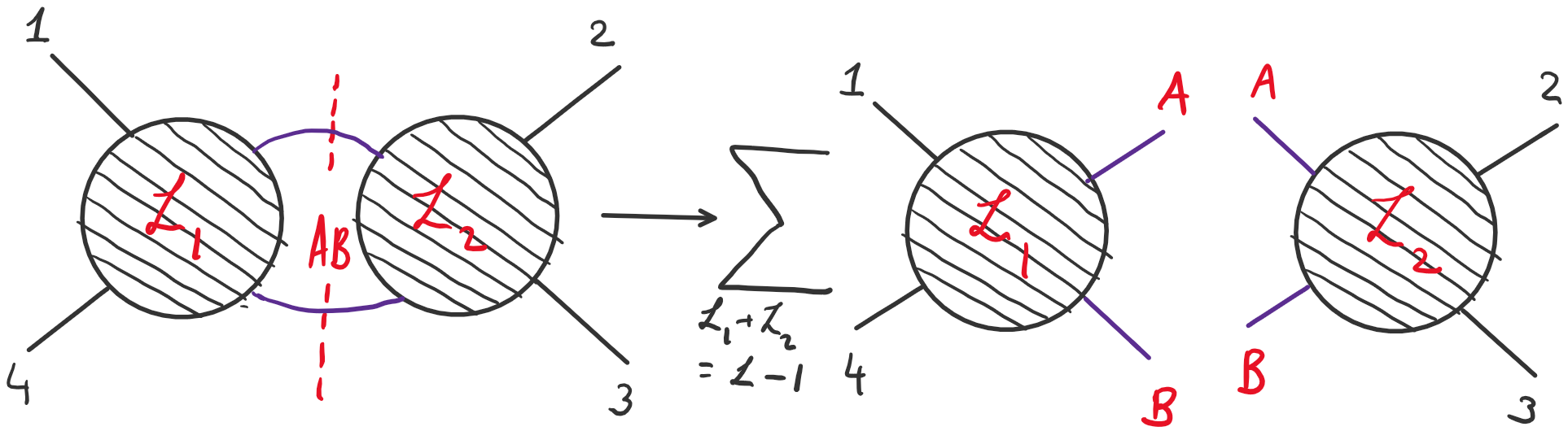 Figure 1
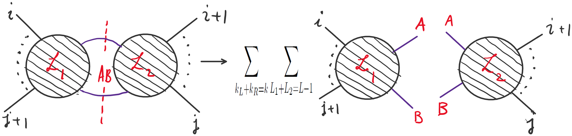 Figure 2
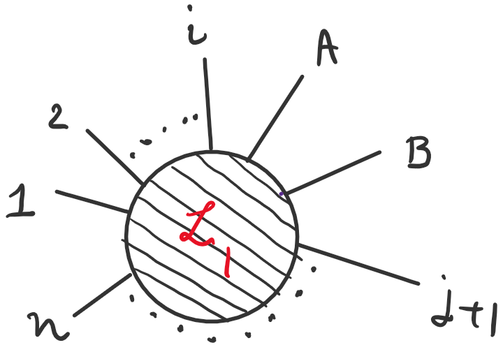 Figure 3
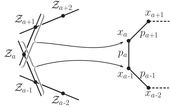 Figure 4
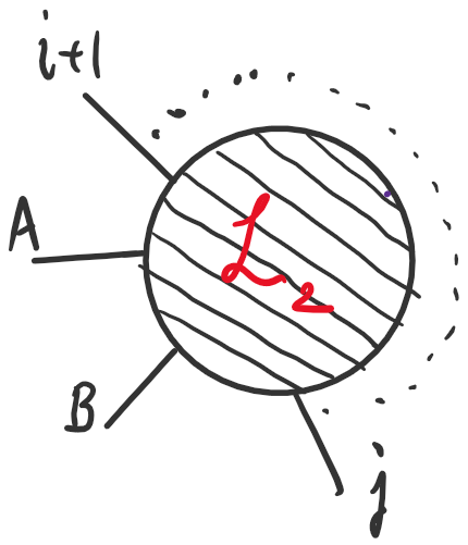 Figure 5
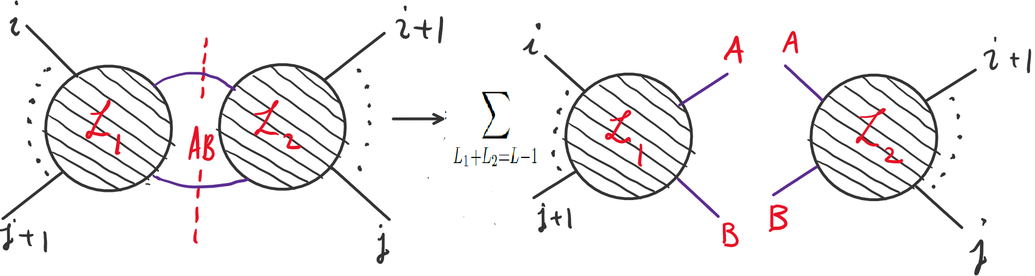 Figure 6
| Region | |||
|---|---|---|---|
| Region | |||
|---|---|---|---|
| + | + | + | 0 |
| + | + | - | 1 |
| + | - | + | -1 |
| + | - | - | 0 |
| - | + | + | -1 |
| - | + | - | 0 |
| - | - | + | 0 |
| - | - | - | 1 |
Peer Reviews
No public reviews on file for this paper yet. If you reviewed it on a platform where reviews are public (OpenReview, ICLR, NeurIPS, ICML), you can paste yours below so the community can read it here.
Videos
No videos yet. Explain this paper in a talk, walkthrough, or lecture? Add one.
††institutetext: Department of Physics, Princeton University, NJ, USA
Emergent Unitarity from the Amplituhedron
Akshay Yelleshpur Srikant
Abstract
We present a proof of perturbative unitarity for planar SYM, following from the geometry of the amplituhedron. This proof is valid for amplitudes of arbitrary multiplicity , loop order and MHV degree .
1 Introduction
Unitarity is at the heart of the traditional, Feynman diagrammatic approach to calculating scattering amplitudes. It is built into the framework of quantum field theory. Modern on-shell methods provide an alternative way to calculate scattering amplitudes. While they eschew Lagrangians, gauge symmetries, virtual particles and other redundancies associated with the traditional formalism of QFT, unitarity remains a central principle that needs to be imposed. It has allowed the construction of loop amplitudes from tree amplitudes via generalized Unitarity methods (unitarity1, ; unitarity2, ; unitarity3, ; unitarity4, ; unitarity5, ) and the development of loop level BCFW recursion relations bcfw1 ; bcfw2 . These on-shell methods have been particularly fruitful in planar SYM and led to the development of the on-shell diagrams in onshelldiagrams and the discovery of the underlying Grassmannian structure. Locality and unitarity seemed to be the guiding principles which dictated how the on-shell diagrams glued together to yield the amplitude. The discovery of the amplituhedron in amplituhedron , intotheamplituhedron revealed the deeper principles behind this process - positive geometry. Positivity dictated how the on-shell diagrams were to be glued together. The resulting scattering amplitudes were miraculously local and unitary!
This discovery of the amplituhedron was inspired by the polytope structure of the six point NMHV scattering amplitude, first elucidated in (hodges, ) and expanded upon in polytopes . This motivated the original definition of the amplituhedron which was analogous to the definition of the interior of a polygon. The tree amplituhedron was defined as the span of planes , living in dimensions. Here and .
[TABLE]
where are positive external data in dimensions. In this context, positivity refers to the conditions if and . is the positive Grassmannian defined as the set of all matrices with ordered, positive minors. For more details on the properties of the positive Grassmannian, see onshelldiagrams ; grassmannian1 ; grassmannian2 ; grassmannian3 and the references therein. The scattering amplitude can be related to the differential form with logarithmic singularities on the boundaries of the amplituhedron. The exact relation along with the extension of eq.(1) to loop level can be found in amplituhedron .
The amplituhedron thus replaced the principles of unitarity and locality by a central tenant of positivity. Tree level locality emerges as a simple consequence of the boundary structure of the amplituhedron, which in turn is dictated by positivity. The emergence of unitarity is more obscure. It is reflected in the factorization of the geometry on approaching certain boundaries. This was proved for in intotheamplituhedron . The extension of this proof to amplitudes with arbitrary multiplicity using (1) is cumbersome and requires the use of the topological definition of the amplituhedron introduced in binarycode . In the following section, we review this definition in some detail along with some properties of scattering amplitudes relevant to this paper. We also expound the relation between the amplituhedron and scattering amplitudes. The rest of the paper is structured as follows. In Section [3], we present a proof of unitarity of scattering amplitudes for 4 point amplitudes of planar SYM, using the topological definition of the amplituhedron. This serves as a warm up to Section [4] in which we provide a proof which is valid for MHV amplitudes of any multiplicity. Finally, in Section 5 we show how the proof of the previous section can be extended to deal with the complexity of higher sectors.
2 Review of the topological definition of
The scattering amplitudes extracted from the amplituhedron defined as in (1), using the procedure outlined in amplituhedron , reproduce the Grassmannian integral form of scattering amplitudes presented in grassmannian1 ; grassmannian2 ; grassmannian3 ; grassmannian4 ; grassmannian5 . These necessarily involve the auxiliary variables . In contrast, the topological definition of the amplituhedron can be stated entirely in terms of the momentum twistors (first introduced in hodges ). Consequently, this yields amplitudes that can be thought of as differential forms on the space of momentum twistors. In this section, we will review the basic concepts involved in the topological definition of the amplituhedron. We begin with a review of momentum twistors and their connection to momenta in Section [2.1] and proceed to the topological definition of the amplituhedron in Section [2.2]. We then explain how amplitudes are extracted from the amplituhedron in Section [2.3] and finally, in Section [2.4], we set up the statement of the optical theorem in the language of momentum twistors. This is the statement we will prove in the main body of the paper.
2.1 Momentum twistors
Momentum twistor space is the projective space . A connection to physical momenta can be made by writing them in the coordinates of an embedding as . Here are the spinor helicity variables which trivialize the on-shell condition.
[TABLE]
where the dual momenta are defined via and trivialize conservation of momentum. Thus the point in dual momentum space is associated to a line in momentum twistor space. Scattering amplitudes in SYM involve momenta which are null and are conserved . Momentum twistors are ideally suited to describe the momenta involved in these amplitudes because they trivialize both these constraints. Figure 1 summarizes the point-line correspondence between points in dual momentum space and lines in momentum twistor space.
Thus all the points of the form
[TABLE]
are associated to the momentum . Note that these are different from the calligraphic used in 1(the connection between the two is that are obtained by projecting the through the plane in 1). Thus, a set of on-shell momenta satisfying can be represented by an ordered set of momentum twistors . Each line corresponds to the point in dual momentum space as shown in Fig 1.
Each loop momentum can also be associated to a line in momentum twistor space. We denote these lines by , where and are any representative points. This helps us distinguish loop momenta from other external momenta. We can express Lorentz invariants in terms of determinants of momentum twistors using the relation
[TABLE]
with and where is the infinity twistor (LocalIntegrands, ; grassmannian2, ). Finally, we connect the invariants involving the with the four bracket via
[TABLE]
We will utilize this connection later in Section [5.4].
2.2 Topological definition
The amplituhedron is a region in momentum twistor space which can be cut out by inequalities. The region depends on the integers and which specify the point, NkMHV amplitude. is the number external legs of the amplitude and correspondingly the number of momentum twistors which are involved in the definition of the amplituhedron. We denote these by . is the number of loops and we have the lines, corresponding to the loop momenta . appears below in the inequalities that define .
2.2.1 Tree level conditions
The first set of conditions that define the amplituhedron involve only the external momentum twistors and we refer to these as the “tree-level” conditions. They are listed below along with some comments about each condition.
- •
The external data must satisfy the following positivity conditions.
[TABLE]
We adopt an ordering in all definitions. We must also define a twisted cyclic symmetry for this ordering with
[TABLE]
This definition is required to ensure that for odd and for even . We will see below that this is crucial to obtain the right number of sign flips.
- •
We require that the sequence
[TABLE]
Note that the ordering is crucial for the above condition to make sense. Using (4), (6) and the reasoning in Appendix [A], we can conclude that all sequences of the form
[TABLE]
with have sign flips. The use of (5) is crucial in arriving at this conclusion. Since all the sequences have the same number of flips (with the appropriate twisted cyclic symmetry factors), we can use any of them in place of the sequence . In the rest of the paper, we will the sequence which is most convenient to the situation.
2.2.2 Loop level conditions
The next set of conditions involve both the external data and the loops and we refer to these as “loop level” conditions.
- •
Each loop must satisfy a positivity condition analogous to (4)
[TABLE]
Note that we must include the twisted cyclic symmetry factor here as well. Once again, this implies that for odd and for even .
- •
We require that sequence
[TABLE]
Following a line of reasoning similar to that in 2.2.1, we can show that all sequences of the form
[TABLE]
with have the same number of sign flips. We will make use of these sequences as convenient in the rest of the paper.
2.2.3 Mutual positivity condition
The final condition is a relation involving multiple loop momenta . We must have
[TABLE]
For multi loop amplitudes, the conditions above amount to demanding that each loop is in the one-loop amplituhedron (i.e. it satisfies conditions and ) and also the mutual positivity condition (9). Finding a solution to all these inequalities is tantamount to computing the point NkMHV amplitude. The complexity of solving the mutual positivity condition shows up even in the simplest case of . Indeed, its solution is at the heart of the four point problem, as explained in intotheamplituhedron .
The topological definition is well suited to exploring cuts of amplitudes (which correspond to saturating some of the inequalities in (4) - (9) by setting them to be equal to zero). This formalism has been exploited to investigate the structure some cuts of amplitudes that are inaccessible by any other means. The results of some classes of these “deep” cuts are obtained to all loop orders in mypaper1 ; mypaper2 .
2.3 Amplitudes and integrands as Canonical Forms
The inequalities (4) - (9) define a region in the space of momentum twistors. The goal of the amplituhedron program is to be able to obtain the amplitude from purely geometric considerations. More precisely, we can obtain the tree level amplitude and the loop level integrand for planar SYM. In contrast to generic quantum field theories, the planar integrand in SYM is a well defined, rational function as shown in unitarity6 ; bcfw2 . The conjecture here is that the Canonical form associated to the amplituhedron is the loop integrand. The Canonical form associated to a region is the differential form with logarithmic singularities on all the boundaries of that region. For more details on Canonical forms, their properties and precise definitions, see canonicalforms . The discovery of amplituhedron-like geometric structures (for e.g. othergeometries1 ; othergeometries2 ; othergeometries3 ; othergeometries4 ) in other theories lends further support to the idea that amplitudes can be thought of as differential forms on kinematic spaces. Some consequences of this are explored in ampsasdiff . It is interesting to note that a topological definition of the amplituhedron has been found directly in momentum space amplituhedronmomentum . This allows for the possibility of expressing SYM amplitudes as differential forms in momentum space rather than momentum twistor space.
It is illustrative to show the calculation of the canonical form for the simple case of . This canonical form should be the 4-point, one-loop MHV integrand. The defining inequalities are
[TABLE]
Since , we can expand these in a basis consisting of . However, are arbitrary points on the line which corresponds to the loop momentum. Since any linear combination of the points and is also on the same line, there is a redundancy in the choice of and . Fixing this redundancy, we arrive at the following parametrization.
[TABLE]
The solution to the inequalities in (10) is
[TABLE]
The boundaries are located at and the differential form with logarithmic singularities on all the boundaries is just
[TABLE]
This is the integrand for the 1-loop four point MHV amplitude as conjectured.
At higher points, the situation is more complicated cases. There are multiple ways in which the sequence (8) can have sign flips. It is useful to triangulate the complete region by enumerating all such patterns. This procedure works extremely well for point MHV amplitudes and is fleshed out in Section [7] of binarycode . Specifically, if we parametrize
[TABLE]
with , we have and . The sequence has two sign flips, one occurring between and and the second between and . Summing over all covers all the positions of the flips. The canonical form for this region is the integrand of the point MHV amplitude.
[TABLE]
For another derivation of this integrand, please refer to bcfw2 .
Finally, an important property of these forms is that they are all projectively well defined. They are invariant under the re-scaling of each external leg. We will make use of this property in Section [5].
2.4 Unitarity and the Optical theorem
The relationship between the singularity structure of scattering amplitudes and unitarity has been the subject of a lot of work. unitarity1 ; unitarity2 ; unitarity3 ; unitarity4 ; unitarity5 ; unitarity6 ; unitarity7 ; unitarity8 ; unitarity9 . It is well known that the branch cut structure of amplitudes is intimately tied to perturbative unitarity. This is encapsulated in the optical theorem which related the discontinuity across a double cut to the product of lower loop amplitudes.
The presence of branch points in loop amplitudes is due to the pole structure of the integrand. This is governed by the boundary structure of the amplituhedron. The structure of boundaries and their relation to branch points has been studied extensively in boundary1 ; boundary2 ; boundary3 ; boundary4 ; boundary5 ; boundary6 ; boundary7 ; boundary8 . The discontinuity across a branch cut is calculated by the residue on an appropriate boundary of the amplituhedron. The optical theorem thus translates into a statement about the factorization of the residue on this boundary. We expect this factorization to emerge as a consequence of the positive geometry.
Let us begin by rewriting the optical theorem, specifically for SYM in the language of momentum twistors. For now, we will focus on MHV amplitudes. We are interested in the case where one of the loops, , cuts the lines and and all other loops (which we denote by ) remain uncut. Thus we are calculating the residue of the MHV amplitude on the cut . It is convenient to parametrize as
[TABLE]
where is an arbitrary reference twistor. The terms in the -loop integrand which contribute to this cut (which has the required poles) can be written as
[TABLE]
The dependence of on the external twistors has been suppressed. The residue of on the cut is
[TABLE]
where is a Jacobian which is irrelevant to our purposes. Unitarity predicts that the function is related to lower point amplitudes (see figure 2) and is of the form
[TABLE]
We will show that this structure emerges from the geometry of the amplituhedron. We will first present a proof for the four point case. This is just a rewriting of the proof found in intotheamplituhedron using the topological definition. This proof will then admit a generalization to amplitudes of higher multiplicity.
3 Proof for 4 point Amplitudes
In this section we will examine the unitarity cut , at four points and show that the residue can be written as a product of lower loop, 4-point amplitudes. Specifically, we will show that the defining conditions of the amplituhedron (4) - (8) can be replaced by two disjoint set of conditions which define a “left amplituhedron” with external data and a “right” amplituhedron with external data . We will show that the mutual positivity conditions in (9) which seemingly connect the “left” and “right” amplituhedra are automatically satisfied once the defining conditions for the “left” and “right” amplituhedra are met. This suffices to prove that the canonical form on the cut is
[TABLE]
where and are the canonical forms of the “left” and “right” amplituhedra respectively. A suitable parametrization of is
[TABLE]
This ensures the cut conditions are satisfied. To compute the canonical form on the cut, we must solve the remaining inequalities. The tree level constraints (4), (6) trivially imply . The remaining loop level conditions in (7) and (8) impose and which ensure . Denoting the uncut loops as with , the remaining inequalities are loop positivity conditions,
[TABLE]
mutual positivity among the uncut loops
[TABLE]
and mutual positivity with the cut loop
[TABLE]
Here we have used the parametrization for and . The consequences of this inequality are best understood by considering the related quantity . Using for and , we can rewrite this as follows.
[TABLE]
The above equation implies as each term on the right hand side is individually positive due to (16) and (18). The two possible solutions are
[TABLE]
and
[TABLE]
A particular loop may satisfy either (20) or (21). In a generic case, there will be loops, which obey and loops, which obey . There are no restrictions on what values and can take. Consequently, the complete region satisfying the inequalities (16) and (18) is a sum over all values of and with . We will now show that the canonical form for a region with fixed and can be written as a product of forms for amplituhedra and . From Fig. 3, it is clear the the external data corresponding to the left amplitude is the set . Any loops which belongs to this amplituhedron must satisfy the defining conditions 4, 6, 7, 8.
[TABLE]
The flip condition is the only one left to be verified and follows from the Plcker relation
[TABLE]
This can be derived by noting that the 5 twistors are linearly dependent which leads to the condition
[TABLE]
Contracting this with yields (23). Note that the RHS of is negative since while the signs of the terms in the LHS are
[TABLE]
This forces and ensures that the sequence in (22) has 2 flips.
Similarly, the external data for the right is the set and a loop which belongs to it satisfies the following conditions.
[TABLE]
Clearly, the conditions (22) and (25) define the amplituhedra and with canonical forms and respectively. To complete the proof that the canonical form on the cut is just the product of these forms, we must show that that mutual positivity between the loops and imposes no further constraints. To see this, we can expand the loop in terms of
[TABLE]
and compute which yields,
[TABLE]
The positivity of all the terms except for and immediately follows from (25). For these two, we have
[TABLE]
Therefore, imposes no new constraints and the canonical form on the cut factorizes into and .
4 Proof for MHV amplitudes of arbitrary multiplicity
We will extend the above results to amplitudes of arbitrary multiplicity. However, the existence of higher sectors beginning with complicates the proof. In this section we will focus on a proof of unitarity for MHV amplitudes. This allows us to sketch the essentials of the proof without additional complications. In the next section, we modify the proof to account for higher sectors.
We are examining the residue of the MHV amplituhedron on the cut . For the rest of the paper, we will assume 111In the singular case of , the amplitude factorizes into a 3-point MHV or amplitude a point MHV amplitude. The 3 point case is degenerate and the use of momentum twistors ensures that all the defining conditions(on-shell and momentum conservation) are always satisfied. There are no further constraints that need to be imposed. The defining conditions for the amplituhedron are
[TABLE]
Here, . We have chosen to look at the flip pattern of a particularly convenient sequence. All other related sequences will also have the same number of flips as mentioned in Section [2.2.2].
There are clearly many patterns of signs for which the sequences has two sign flips. We refer to each pattern as a configuration of the amplituhedron. A configuration for the MHV amplituhedron is specified by giving the signs of all entries of the sequence S. We would like to show that for each configuration, the canonical form can be written as the product of canonical forms of a left and right amplituhedron. To begin, we we can parametrize the cut loop as
[TABLE]
To show that the canonical form on this cut can written as a product of canonical forms for lower loop, “left” and “right” MHV amplituhedra and (with ), we need precise definitions of these objects. This is provided in the following section.
4.1 Left and right Amplituhedra
4.1.1 The left amplituhedron
The left amplituhedron is defined by three sets of conditions similar to . In this case, the external data, as seen from Fig 4 is the set . Letting denote elements of this set and , the defining conditions are
[TABLE]
These are satisfied if and .
[TABLE]
The above sequence lends itself to easy comparison with the sequence in (27). However, for consistency, we must also verify that the following sequences have the same number of sign flips as .
[TABLE]
This ensures that the definition of the amplituhedron is independent of the choice of sequence, similar to Section [2.2.2]. The positivity conditions on the loop data ensures that all the first and last entries of these sequences are positive. Furthermore any two sequences in the above set, all of which are of the form and , satisfy
[TABLE]
The equality of sign flips now follows from the analysis in Appendix . This shows that the left amplituhedron can be consistently defined at tree level. The mutual positivity and the loop level positivity conditions for all the loops in the left amplituhedron are automatically satisfied because of and . The flip condition defines the criterion for any uncut loop to be in the left amplituhedron. We will present a detailed analysis in Section [4.2].
4.1.2 The right Amplituhedron
The external data for the right amplituhedron is and the defining inequalities are listed below. and with being an uncut loop.
[TABLE]
Once again, for consistency we should verify that
[TABLE]
all have the same number of sign flips as . The proof is identical to the one for the left amplituhedron. The tree level, mutual positivity and loop level positivity conditions are once again guaranteed by and and an analysis of the flip condition is in Section [4.2].
4.2 Factorization on the unitarity cut
It was shown in the last section that the two sets and define positive external data and that the loop level positivity conditions are satisfied. We need to analyze every configuration of the amplituhedron and show that for each configuration, an uncut loop belongs to the left or the right amplituhedron. The similar analysis for the 4 point case, performed in Section [3], was much simpler owing to the fact there there was only one possible sign pattern for the sequence, . Here, the presence of multiple compatible sign patterns increases the complexity of the proof and no simple relation like (3) exists. It is natural to label the configurations of by looking at the sign patterns in the sequence S as explained below.
[TABLE]
Note that the flip pattern of this sequence determines whether the loop belongs to the original amplituhedron which has external data . Consequently, it doesn’t involve the points and . We have divided the sequence in a suggestive way. The half of looks very similar to (4.1.2). It is natural to label the different flip patterns of as where are the signs of and and are the number of flips in the left and right parts of .
In order to compare (4.1.1) to , we introduce the sequence
[TABLE]
and call the number of flips in this sequence flips. The motivation behind introducing this is that and are connected by the Plcker relation (similar to (29))
[TABLE]
Following the analysis in Appendix[A], the relation between and is determined entirely by the signs of the first and last elements
[TABLE]
where is the number of sign flips in . If , then otherwise .
now looks almost like a juxtaposition of and . Each flip pattern of S determines whether the corresponding loop belongs to the left or the right amplituhedron as shown below.
- •
The sequence clearly has 2 sign flips since
[TABLE]
has one sign flip since
[TABLE]
Furthermore and the loop belongs only to the right amplituhedron.
- •
obviously has [math] sign flips. If , and if , . In both cases, the loop belongs to the left amplituhedron and not the right.
- •
If , then the sequence has 0 flips and the loop doesn’t belong to the right amplituhedron. If , and . Otherwise, and . Thus irrespective of the sign of , the loop belongs to the left amplituhedron.
If , then has 2 sign flips and it can be shown that by analysis similar to the cases above. This belongs to the right amplituhedron.
- •
In this case, has two flips and has one flip irrespective of the sign of . Since , we have and the loop belongs to the right amplituhedron.
- •
Once again, it is simple to show that has two sign flips and has 0 sign flips in this configuration.
4.2.1 Trivialized mutual positivity
We have shown that for every configuration of the amplituhedron, each loop belongs either to the left or the right. While we can consistently define left and right amplituhedra, it remains to be shown that the mutual positivity between a loop in the left amplituhedron and a loop in the right amplituhedron doesn’t impose any extra constraints.
This is easiest to see if we expand each loop and using (11) as
[TABLE]
with and . On expanding , every term is of the form with . Since the external data are positive, i.e. for , we are assured that .
This completes the proof of factorization for MHV amplituhedra on the unitarity cut. In the next section, we will extended this proof to the higher sectors.
5 Proof for higher sectors
The proof of unitarity for higher is similar in spirit to that for the MHV sector. However, there are a lot additional details that we must take into account. Firstly, we must modify (14) to include products of “left” and “right” amplituhedra with different . Suppose the left amplitude has negative helicity gluons and the right amplitude has negative helicity gluons, then we have . With the MHV degrees defined as , this equation reads . Recall that we introduced the function in (13) and stated the optical theorem in terms of it. Including sectors of different , this becomes,
[TABLE]
We expect that unitarity emerges from a factorization property of the geometry in a manner similar to the MHV case. In order to make this statement more precise, we will have to define analogues of the left and right MHV amplituhedra for NkMHV external data. , the MHV amplituhedron defined by the conditions
[TABLE]
We can use any sequence instead of as explained in Section [2.2.2].
It is worth re-emphasizing that we wish to prove that the canonical form on the cut (which is computed by solving the inequalities (5) for the uncut loops along with ) can be written as in (33). For this to happen, we want to show that the set of inequalities in (5) can be replaced by two sets of inequalities which define lower loop amplituhedra, and . It is not essential that the external data for these is a subset of . In particular they can be rescaled by factors and still yield the same canonical form due to projective invariance as discussed in Section [2.3]. In fact, as we show below, this rescaling plays a crucial role in ensuring that the left and right amplituhedra have of both even and odd parity.
On the unitarity cut ( with ), there is a natural division of the external data into “left” and “right” sets, and . However, insisting that this be the external data for the left and right amplituhedra imposes too many constraints. To see this, suppose that the “left” set has MHV degree . We must have . But (5) implies that . This forces and restricts to be the same parity as . Similarly for the right set, we have and again (5) implies which forces . In order to avoid these extra constraints on and , we must allow for arbitrary signs on the and define two the sets of external data as
[TABLE]
where . These signs will be determined by conditions like which define the left and right amplituhedra along with the appropriate twisted cyclic symmetry. We will then show that the canonical form for every configuration in can be mapped into a product of canonical forms on suitably defined left and right amplituhedra and .
5.1 The left and right amplituhedra
5.1.1 The left amplituhedron
We must demand that the set satisfies all the conditions in . In addition, this must also be compatible with the fact that the are the external data for .
[TABLE]
and the automatically satisfy and . Thus we have, and . Furthermore, we have new constraints on and coming from
[TABLE]
Finally, since the set is the external data for , it must satisfy a twisted cyclic symmetry
[TABLE]
Since , consistency requires . This divides into two cases
- •
An allowed set satisfying and is
[TABLE]
with and undetermined. requires and the constraints in read
[TABLE]
The solutions to these constraints are
[TABLE]
- •
In this case satisfying and is
[TABLE]
which again requires and turns into
[TABLE]
This has the following solutions
[TABLE]
Each of these regions is characterized by particular signs for and along with a pattern of sign flips for the sequence
[TABLE]
Each region allows parametrization of the line as and with . In the table below, we list the different possibilities.
It is crucial to remember that the canonical form is independent of the choice of and parametrization of and . In all these cases the canonical form is that of .
5.1.2 The right amplituhedron
A similar analysis of the effects of on the set yields the following constraints on .
[TABLE]
These conditions are satisfied by
[TABLE]
with and having solutions depending on .
- •
[TABLE]
- •
[TABLE]
Once again, each region is characterized by different pattern of sign flips of the sequence
[TABLE]
where we have ignored an overall factor of . We list the various parametrizations and sign patterns of below.
The canonical form is independent of the choice of and parametrization of and .
5.2 Factorization of the external data
We will show that, on the unitarity cut, for every allowed sign flip pattern of the sequence , there exist regions such that and have the flip patterns necessary for and . The analysis that follows is similar to the one is Section [4.2]. The sequence is similar to the left part of and can be compared directly. In order to compare with , it is necessary to introduce another sequence . This is analogous to what we did in (31).
[TABLE]
Let be the number of flips in respectively. and are related to each other due to the following Plcker relations
[TABLE]
and
[TABLE]
It is easy to see that these hold in all regions . As shown in Appendix[A], we can conclude that the relation between and depends only on the signs of first and last terms which are encoded in the matrix below.
[TABLE]
The relation between and is tabulated below.
It is helpful to label all the allowed flip patterns of as where and are the signs of and respectively. The different possibilities are shown below.
[TABLE]
For each configuration, , the sequences and have the following signs depending on the region .
For the configuration , we have . Thus regions which satisfies are .
For the configuration , we have . Thus regions which satisfies are .
For the configuration , we have . Thus regions which satisfies are .
For the configuration , we have . Thus regions which satisfies are .
We see that for every configuration , there are regions that satisfy . Thus every configuration in the original amplituhedron can be covered by these regions consistent with the expected factorization. The remaining regions exist because they are related to amplitudes via inverse soft factors and have identical canonical forms. However, these are not necessary to cover all regions of the original amplituhedron.
5.3 Factorization of loop level data
At loop level, we need to show that each loop belongs either to the left or the right amplituhedron. The relevant sequences are (denoting as )
[TABLE]
Similar to before, it will be convenient to introduce the sequence
[TABLE]
Let the number of flips in and be and respectively. These are not and , which are the number of flips in the tree level sequences and respectively. The flip patterns of S can be organized as follows.
[TABLE]
We showed in the previous section that on the unitarity cut, the external data factorizes such that with . It is trivially true that each loop belongs either to the left or the right amplituhedron. We must show that if a loop belongs to the left amplituhedron, then it cannot belong to the right amplituhedron. First, note that in each configuration, we will have and with or . Now suppose that belongs to both the left and right amplituhedra. Then we must have and . Expressing and in terms of and , and using , we get
[TABLE]
Clearly, is impossible since or . We just need to show that is impossible. Note that this is possible only if . In this case, the following hold true.
[TABLE]
[TABLE]
In all these cases, we must have . It is easy to verify from Section [5.1] that this is always false. Thus each loop belongs solely to the left or the right ampltuhedron.
5.4 Mutual positivity
To complete the proof of factorization, we need to show that the mutual positivity between a loop in and one in is automatically satisfied. This is easier to see while working with dimensional data. We can re-write all the four brackets using and the plane as described in Section [2.1]. For more details, see Section [7] of binarycode . A loop in the left amplituhedron can be parametrized as a plane .
[TABLE]
with , and .
Similarly, a loop in the right amplituhedron can be thought of as a plane and parametrized as
[TABLE]
with , and with .
This reduces the mutual positivity condition to a condition involving brackets of the form . It is easy to see that with positive dimensional data when , mutual positivity is guaranteed. The signs and are crucial in making this work.
6 Conclusions
We have shown that unitarity can be an emergent feature. The positivity of the geometry inevitably leads to amplitudes identical to those derived from a unitary quantum field theory. This lends further support for the conjecture that the amplituhedron computes all the amplitudes of SYM. It also suggests that the notion of positivity is more fundamental than those of unitarity and locality which are the cornerstones of the traditional framework of quantum field theory.
Acknowledgements.
We would like to thank Nima Arkani-Hamed and Jaroslav Trnka for useful discussions and comments about the manuscript.
Appendix A Restricting flip patterns
Consider a pair of sequences and which have an equal number of terms. Further suppose that they are connected by the Schouten identity and satisfy a postivity condition, i.e. there exists a relation . We will show that the number of sign flips in these sequences, and respectively, are related and that the relation depends only on the signs of and .
Firstly, we note that the positivity forces each block in the pair of sequences to take one of the following forms.
[TABLE]
Blocks of type 1 and 2 leave fixed. A block of type 3 changes by and a block of type 4 changes it by . Two consecutive blocks of type 3 or 4 are prohibited and a block of type 4 must follow a block of type 3 before the sign of the bottom sequence can be flipped without flipping the sign of the top. Thus, if we know the signs of and , we can determine . We can list the possibilities by the matrices where is the sign of .
- •
[TABLE]
- •
[TABLE]
- •
[TABLE]
The reference list from the paper itself. Each links out to its DOI / PubMed record.
- 1[1] Z. Bern, J. J. M. Carrasco, L. J. Dixon, H. Johansson, and R. Roiban. Manifest ultraviolet behavior for the three-loop four-point amplitude of 𝒩 = 8 𝒩 8 \mathcal{N}=8 supergravity. Phys. Rev. D , 78:105019, Nov 2008.
- 2[2] Charalampos Anastasiou, Ruth Britto, Bo Feng, Zoltan Kunszt, and Pierpaolo Mastrolia. d-dimensional unitarity cut method. Physics Letters B , 645(2):213 – 216, 2007.
- 3[3] Ruth Britto, Freddy Cachazo, and Bo Feng. Generalized unitarity and one-loop amplitudes in n=4 super-yang–mills. Nuclear Physics B , 725(1):275 – 305, 2005.
- 4[4] Zvi Bern, Lance Dixon, David C. Dunbar, and David A. Kosower. Fusing gauge theory tree amplitudes into loop amplitudes. Nuclear Physics B , 435(1):59 – 101, 1995.
- 5[5] Zvi Bern, Lance Dixon, David C. Dunbar, and David A. Kosower. One-loop n-point gauge theory amplitudes, unitarity and collinear limits. Nuclear Physics B , 425(1):217 – 260, 1994.
- 6[6] Ruth Britto, Freddy Cachazo, and Bo Feng. New recursion relations for tree amplitudes of gluons. Nucl. Phys. , B 715:499–522, 2005.
- 7[7] Nima Arkani-Hamed, Jacob L. Bourjaily, Freddy Cachazo, Simon Caron-Huot, and Jaroslav Trnka. The All-Loop Integrand For Scattering Amplitudes in Planar N=4 SYM. JHEP , 01:041, 2011.
- 8[8] Nima Arkani-Hamed, Jacob L. Bourjaily, Freddy Cachazo, Alexander B. Goncharov, Alexander Postnikov, and Jaroslav Trnka. Grassmannian Geometry of Scattering Amplitudes . Cambridge University Press, 2016.