Signatures of Topological Phonons in Superisostatic Lattices
Olaf Stenull, T. C. Lubensky

TL;DR
This paper investigates how topological surface phonons in idealized lattices manifest as finite-frequency modes in realistic superisostatic lattices, with implications for designing mechanical metamaterials.
Contribution
It introduces a study of finite-frequency topological surface phonons in superisostatic lattices with added interactions, bridging ideal models and real-world materials.
Findings
Finite-frequency surface phonons are present in superisostatic lattices.
Signatures of topological modes persist despite added interactions.
Results are relevant for designing mechanical metamaterials.
Abstract
Soft topological surface phonons in idealized ball-and-spring lattices with coordination number in dimensions become finite-frequency surface phonons in physically realizable superisostatic lattices with . We study these finite-frequency modes in model lattices with added next-nearest-neighbor springs or bending forces at nodes with an eye to signatures of the topological surface modes that are retained in the physical lattices. Our results apply to metamaterial lattices, prepared with modern printing techniques, that closely approach isostaticity.
Click any figure to enlarge with its caption.
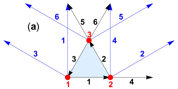 Figure 1
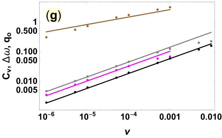 Figure 2
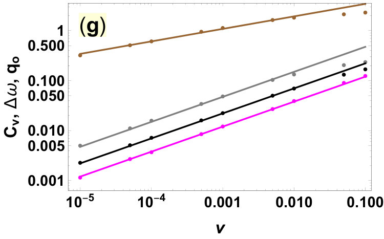 Figure 3
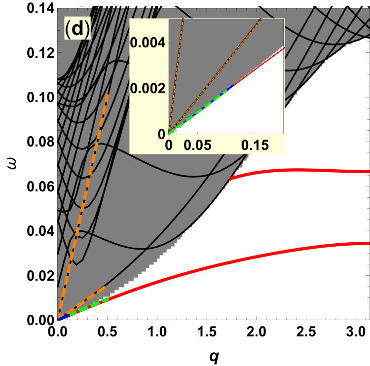 Figure 4
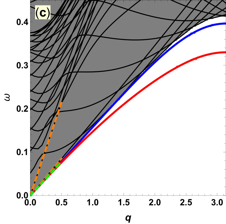 Figure 5
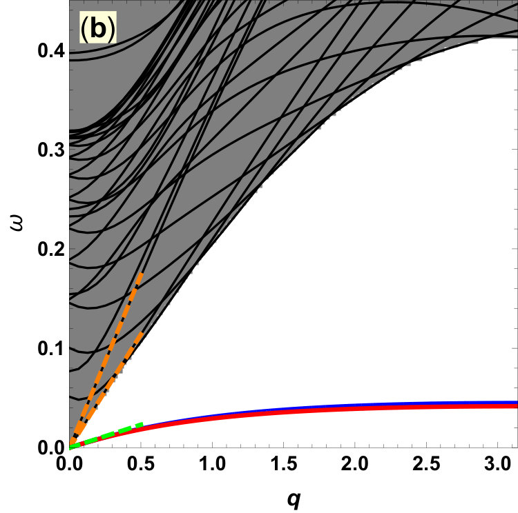 Figure 6
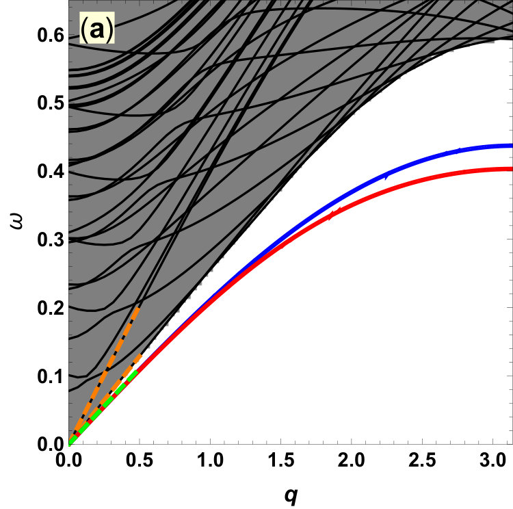 Figure 7
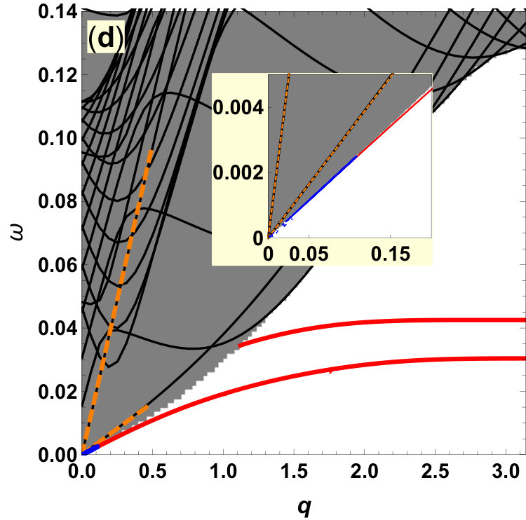 Figure 8
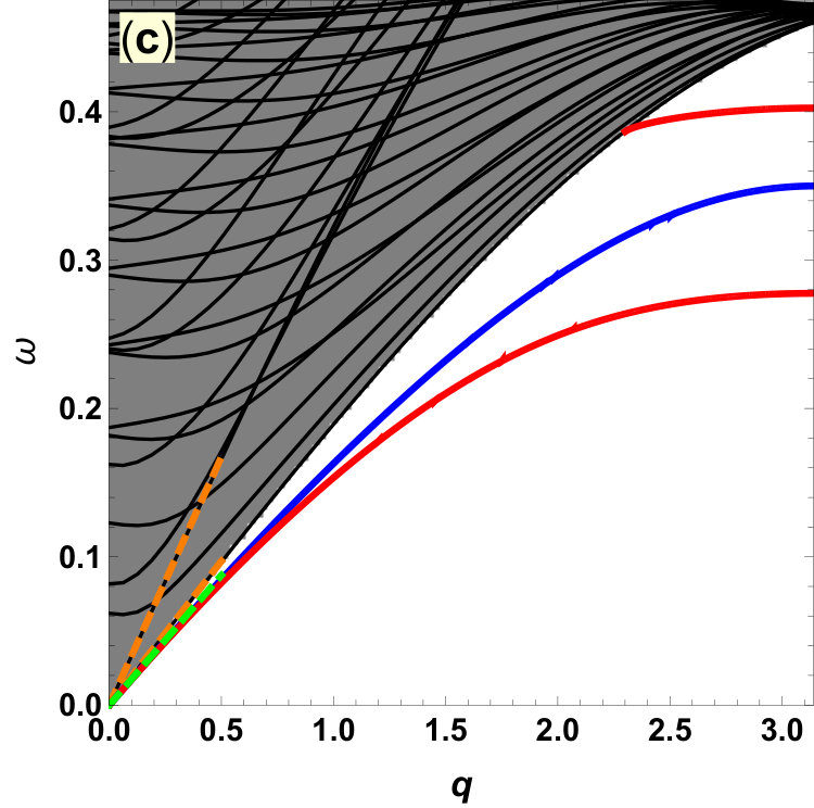 Figure 9
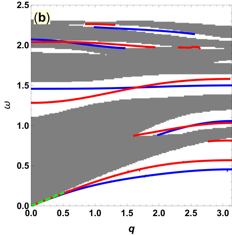 Figure 10
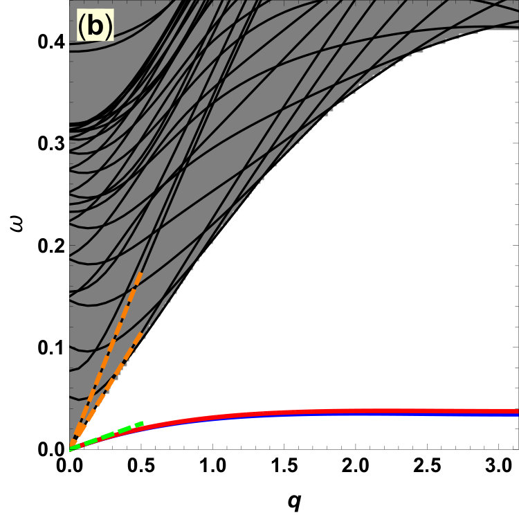 Figure 11
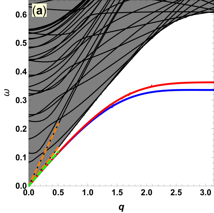 Figure 12
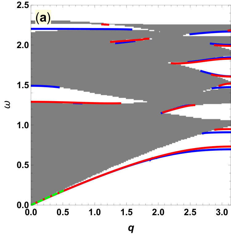 Figure 13
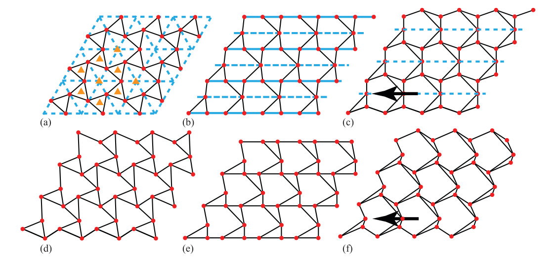 Figure 14
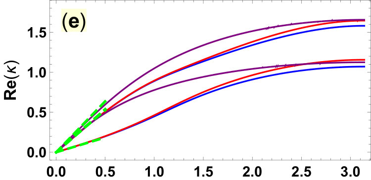 Figure 15
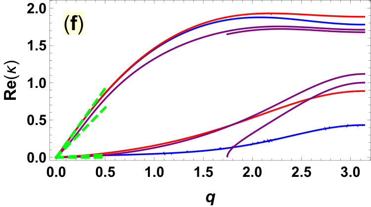 Figure 16
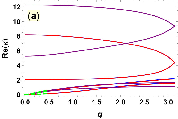 Figure 17
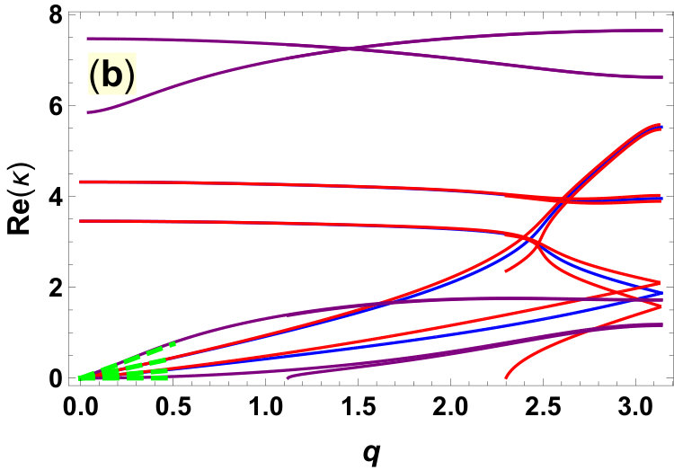 Figure 18
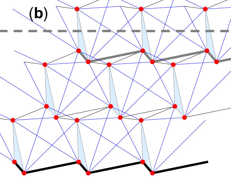 Figure 19
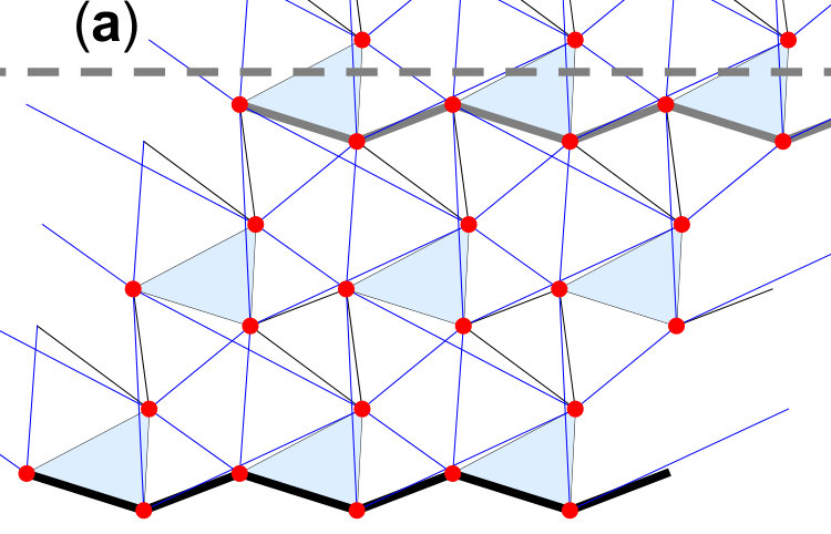 Figure 20
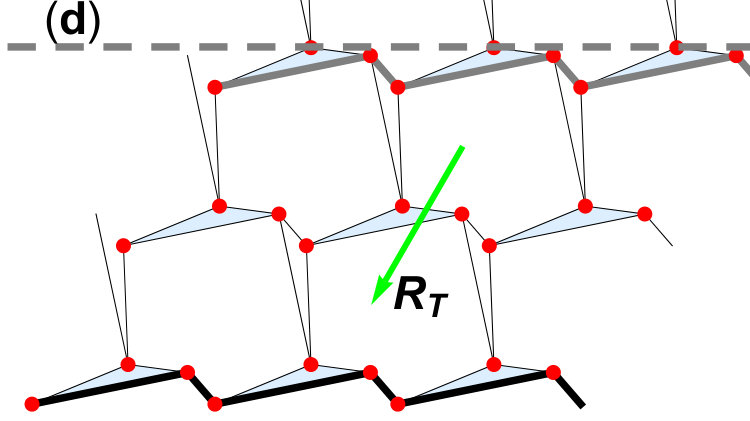 Figure 21
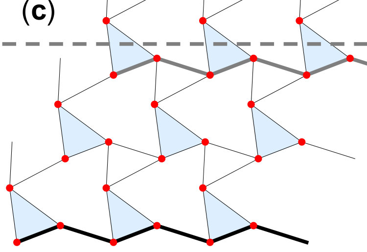 Figure 22
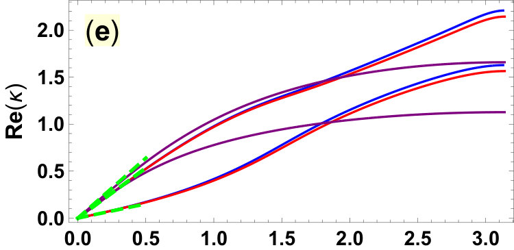 Figure 23
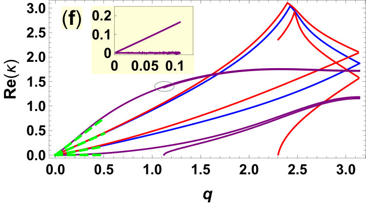 Figure 24
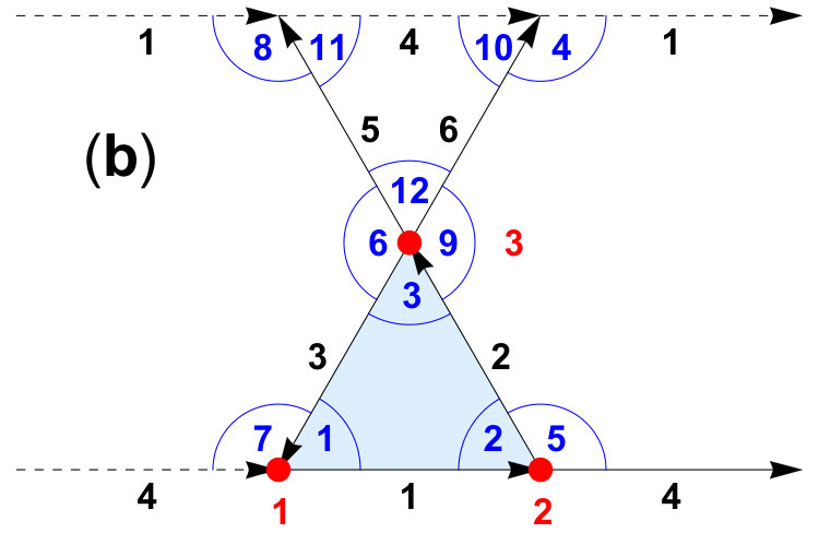 Figure 25
Peer Reviews
No public reviews on file for this paper yet. If you reviewed it on a platform where reviews are public (OpenReview, ICLR, NeurIPS, ICML), you can paste yours below so the community can read it here.
Videos
No videos yet. Explain this paper in a talk, walkthrough, or lecture? Add one.
Signatures of Topological Phonons in Superisostatic Lattices
Olaf Stenull
Department of Physics and Astronomy, University of Pennsylvania, Philadelphia, PA 19104, USA
T. C. Lubensky
Department of Physics and Astronomy, University of Pennsylvania, Philadelphia, PA 19104, USA
Abstract
Soft topological surface phonons in idealized ball-and-spring lattices with coordination number in dimensions become finite-frequency surface phonons in physically realizable superisostatic lattices with . We study these finite-frequency modes in model lattices with added next-nearest-neighbor springs or bending forces at nodes with an eye to signatures of the topological surface modes that are retained in the physical lattices. Our results apply to metamaterial lattices, prepared with modern printing techniques, that closely approach isostaticity.
Recent work Kane and Lubensky (2014); Lubensky et al. (2015); Mao and Lubensky (2018) laid the foundation for a theory, akin to the topological band theory of electronic materials such as quantum Hall systems Halperin (1982); Haldane (1983) and topological insulators Kane and Mele (2005a, b); Bernevig et al. (2006); Moore and Balents (2007); Fu et al. (2007); Hasan and Kane (2010); Qi and Zhang (2011), of topological mechanics of periodic ball-and-spring isostatic lattices with average coordination number , under periodic boundary conditions, equal to twice the spatial dimension, . This theory predicts the existence of zero-energy surface-modes at every surface wavenumber with the number of these modes on different surfaces depending on the topological properties of the bulk phonon spectrum. It has been applied to a variety of systems and phenomena Stenull and Lubensky (2014); Paulose et al. (2015a, b); Sussman et al. (2016); Rocklin et al. (2016); Stenull et al. (2016); Chen et al. (2016); Meeussen et al. (2016); Baardink et al. (2018); Zhou et al. (2018a, b) from random and jammed systems to stress concentration at topological domain walls. Our focus here is on periodic fully gapped systems in which the only bulk zero modes are those imposed by translational invariance at wavenumber . Naturally occurring crystals always have an effective coordination number greater than (because forces between sites have a range greater than the inter-site separation) or stabilizing bending forces favoring particular angles between bonds incident on a given site, and they are not candidates to exhibit topological mechanics. On the other hand, with the aid of modern printing and cutting techniques, metamaterials with consisting of vertices connected by thin nearest-neighbor (NN) elastic beams can be designed Stenull et al. (2016); Baardink et al. (2018) and constructed Bilal et al. (2017); MaZhou2018 to minimize bending forces and, thereby, closely approach the isostatic limit to which the topological theory of Refs. Kane and Lubensky (2014); Lubensky et al. (2015); Mao and Lubensky (2018) applies.
Here we study generalized kagome lattices (GKLs) to which weak next-nearest-neighbor (NNN) springs or bending forces Mao and Lubensky (2011) are added [Fig. 1], and we focus on how their surface modes evolve as the magnitudes of these forces are increased from zero. In the presence of either such force, the originally isostatic lattices become stable elastic materials whose long-wavelength excitations are described by continuum elasticity, which predicts identical Rayleigh waves Landau and Lifshitz (1986) on opposite surfaces of a strip [see Supplemental Material (SM)]. It would be natural to expect that these Rayleigh waves evolve from zero-energy surface modes of the isostatic lattice, and this is indeed the case for non-topological lattices, which have the same number of zero modes on all pairs of opposite parallel surfaces Kane and Lubensky (2014). But this cannot be the case for topological lattices, which have opposite parallel surfaces with different numbers of zero modes –at the extreme no zero modes on one and an associated excess of zero modes on the opposite surface. In what follows, we discuss Rayleigh waves in weakly superisostatic lattices in the context of topological phonons, and we detail how the dilemma posed by the topological lattices is resolved.
For the sake of generality, we consider generic non-topological () and topological () GKLs that have the lowest possible plane crystallographic symmetry, p1. To study surface modes, we assume that a free surface parallel to the -axis exists as indicated in Fig. 1 so that the network as a whole is semi-infinite with a parallel opposite surface located at infinite distance. For the standard GKL with , liberating these two surfaces from the constraints of periodic boundary conditions amounts to removing 2 bonds or 4 bonds and one site per surface unit cell. Both choices lead to two zero-surface-modes per surface wavenumber distributed on the combined lower and upper surfaces, but the latter, which we consider, has smoother upper and lower surfaces as shown in Fig. 1. The topological polarization Kane and Lubensky (2014) calculated from the bulk phonon spectrum is zero for , and it is non-zero and pointing towards the bottom surface, , for . As a consequence, there is one zero-surface-mode per on either surface for and two (zero) zero-surface-modes per on the bottom (top) surface for .
Turning to , we will first review our results and then present some details about how we obtained them. Because of space constraints and for concreteness, we center our discussion on the case with NNN forces. Further details, model elastic energies etc., and results for the case with bending forces are provided in the SM. Figure 2 summarizes our major results about changes in the phonon band structure as the strength of the NNN coupling increases from zero and, in particular, how long-wavelength Rayleigh waves with the same speed develop on opposite surfaces and how the zero-energy surface states at evolve with increasing . At , both and have one acoustic surface mode on each surface at each wavenumber in the surface Brillouin zone (SBZ). At small , the modes reduce to the elastic Rayleigh waves with dispersion on opposite surfaces with the same surface , predicted by elastic theory. The situation at is very similar to that at for except that the acoustic surface-mode frequency is smaller at every , indicating an approach to a single zero mode at each on each surface as . Figure 2 (g) shows that as follows from the observation that must be linearly proportional to some combination of spring constants and be equal to zero at . The situation for is more complex. The bottom surface has an acoustic mode that stretches across the SBZ and reduces to the expected Rayleigh wave at small and, in addition, a low-frequency optical mode whose frequency, is proportional to across the SBZ and that vanishes into the continuum at a critical wavenumber . The top surface, on the other hand, below the lowest bulk band only has a Rayleigh wave with the same velocity as that of the bottom surface, that disappears into the bulk continuum at a wavenumber that vanishes as . The two zero-frequency modes of the topological lattice on the bottom surface are then the limits of the acoustic mode and the low-frequency optical mode. At , the bottom of the band of bulk states, , is proportional to rather than as can be calculated from the envelope of the bulk dispersion, which has the form Kane and Lubensky (2014); Lubensky et al. (2015) at small . Thus equating to yields in agreement with our numerical calculations.
The finite frequency dispersions of surface states in both the and lattices (both with p1 symmetry) depicted in Fig. 2 are in general different on the top and bottom surfaces, as one would expect because opposite surfaces in lattices with such low symmetry are not equivalent. However, consistent with elastic theory, the small Rayleigh waves on both surfaces are the same and do not reflect p1 symmetry. All of the higher frequency modes do however. The high- frequencies of the acoustic modes of both lattices are different on the two surfaces as are all the higher-frequency optical surface modes [see SM].
The approach of the finite-frequency phonons to the topological phonons is also reflected in their inverse penetration depths shown in Figs. 2 (e) and (f). For both and , is the same for at sufficiently small on the bottom and top surfaces as predicted by elastic theory, but differences between the bottom and top surfaces arise as becomes larger. As observed in the dispersion curves, the limit unfolds differently in the two lattices. For , the curves of the two surfaces approach one another as vanishes and eventually become identical across the entire SBZ. For , the curves of the top surface terminate at values of that decrease with whereas the curves of the acoustic and the lowest optical mode on the bottom surface approach each other to produce a two-fold degenerate zero-frequency mode at . Note that the penetration depth of the most dominant contribution to this mode diverges for . The inset to Fig. 2 emphasizes the extremely small (but which we have verified is nonetheless positive) value of throughout the region that the surface acoustic mode exists on the top surface indicating a very large penetration depth.
Our results for the GKL with bending forces are very similar [see SM]. The only notable difference is that the interaction strength is effectively larger than in the NNN model due to factors mandated by the rotational invariance of the bending energies. Apart from that, the approach of the finite-frequency phonons to the topological phonons is qualitatively the same.
We now outline how these results were obtained. The GKLs are derived from the standard kagome lattice (KL) by displacing Kane and Lubensky (2014) the 3 KL unit cell sites , , and by
[TABLE]
where 111Our convention is equivalent to that of Ref. [1,2] with a change in the signs of the ’s, so that the topological polarization is , where are the primitive translation vectors.. are the normalized NN bond vectors of the KL: , , . are unit vectors perpendicular to the : , , . The displacements are designed Kane and Lubensky (2014); Lubensky et al. (2015) so that making one of the ’s nonzero causes filaments (i.e., sample traversing straight lines of bonds) parallel to to zigzag while keeping the remaining filaments straight. The crystallographic symmetry of the resulting GKL depends on . For example, the twisted KL with (where is some reasonable positive or negative number) has p31m symmetry [see SM]. For and , the symmetry is reduced to cm and pm, respectively. Our generic GKLs have deformation parameters and . We have chosen these parameters so that the resulting GKLs have the lowest possible (p1) symmetry, and moderate distortions relative to the KL. Otherwise, these choices are arbitrary, and manifolds of alternative choices lead to qualitatively the same results.
The vibrational modes of an elastic network are governed by its dynamical matrix . In the bulk GKL, the equation of motion is simply , where is the displacement vector of the basis sites, is the wave vector, and is the angular frequency. is the lattice dynamical matrix (for unit mass at sites), with the equilibrium matrix, the compatibility matrix, and the spring constant matrix (see Ref. Lubensky et al. (2015) for background information). In the elastic (continuum) limit, turns into a 2-component displacement field and turns into a effective dynamical matrix. Details about the dynamical matrices in the two theories are given in the SM.
To get a comprehensive picture, we use both lattice and elastic theory. In our elastic theory, we adapt the standard textbook calculation Landau and Lifshitz (1986) of the decay lengths and sound velocities of acoustic surface phonons in isotropic continua to our anisotropic GLKs [see SM]. This approach applies only to the longest wavelength acoustic phonons. Our lattice-based calculations are a generalization to discrete lattices of the standard Rayleigh-wave continuum calculations Landau and Lifshitz (1986). Like the latter calculations, they are done on semi-infinite systems that clearly separate top and bottom surfaces, yet they allow access to wave vectors ranging across the entire SBZ. To carry out our calculations, we break the lattice into one-cell-thick layers , with the surface layer, the next layer into the bulk, and so on, stacked in the -direction and with periodic boundary conditions along . The equilibrium matrix has non-vanishing components and connecting sites in layer to bonds in layers and , respectively; and the compatibility matrix has non-vanishing components and connecting bonds in layer to sites in layers and , respectively. The dynamical matrix then has components , , and . The equation of motion for any layer then reads
[TABLE]
which is solved by provided that
[TABLE]
where is the unit matrix, and determines the the inverse decay length in the -direction via (with in general complex). Solutions of Eq. (3) come in pairs with reciprocal magnitude. Solutions with correspond to bulk modes, whereas solutions with decay away from the bottom (top) surface and correspond to surface modes. The points in --space where bulk modes exist, i.e., points for which there is at least one pair of solutions with magnitude 1, form bands akin to the projected band structures in electronic systems (see Fig. 2). Surface modes can exist only within the bulk band gaps as the solutions of the equations of motion must obey the conditions imposed by the surface. Sites 1 and 2 of the surface unit cell lie directly in the free surface (note that site 3 does not). The force on these surface sites comes only from NN and NNN bonds to [Fig. 1] in the zeroth layer, and as a result for the free boundary condition we impose, the first four components of the force vector satisfy . For , there are a total of eight zeros at any point in --space. This implies that, at any point in a band gap, there are four modes with that decay away from the bottom (top) surface. The boundary conditions can be satisfied by superimposing these decaying modes,
[TABLE]
where the are mode amplitudes and are polarization vectors. The band gap points for which the determinant of the boundary matrix , defined by
[TABLE]
vanishes determine the dispersion relation of the surface modes. To find these points, we use the standard secant-method for computing zeros with an array of starting points that sweeps the band gaps.
Modern printing and cutting techniques now produce bespoke materials, including regular lattices, with almost arbitrary designs. In particular, these techniques can produce mechanical lattices, whose geometry is almost identical to isostatic mechanical NN topological lattices. To fully understand and control these lattices, it is important to know how their properties - elastic energy, bulk- and surface- mode structure, etc. - differ from those of the ideal NN isostatic lattice. Our formalism treats semi-infinite systems exactly and can easily be used to calculate linearized response, for example to a localized force at a surface.
The main result of the present work is the unravelling of the apparent dilemma of topological lattices where topological-phonon theory predicts for the example we are studying two soft surface modes on one surface (soft, bottom) and zero on the other (hard, top) whereas elasticity theory mandates that there be one Rayleigh wave per surface wavenumber on each surface and that the two waves have equal speeds. Our work shows that the resolution of the dilemma is as follows: as , the domain of existence of the Rayleigh wave on the top surface shrinks to zero. On the bottom surface, there is a low-energy optical surface mode, whose domain grows to the full SBZ and which approaches the bottom surface Rayleigh wave as . These two together produce the two surface-zero modes predicted by topological-phonon theory.
Our results provide guidance for interpreting results of experiments on metamaterials targeting topological phonons. Reference MaZhou2018 reports experiments and finite element analysis on kagome-like lattices that show an asymmetric bulk phonon spectrum in a topological lattice but a symmetric one in a non-topological lattice. They verify the existence, in the same geometry we study, of the two low-energy surface modes on the soft surface that emerge from the two zero modes of the ideal topological lattice which they interpret as “an interesting departure from the conventional case of Rayleigh waves”. Curiously neither the finite element analysis nor the measurements show any evidence of the acoustic Rayleigh wave on the hard surface mandated by elasticity theory. It would be interesting to see additional experiments that specifically target the evolution of the hard surface Rayleigh wave with increasing bending rigidity.
Acknowledgements.
This work was supported by the NSF under No. DMR-1104701 (OS, TCL), No. DMR-1120901 (OS, TCL), and No. DMR-1720530 (OS, TCL). TCL was supported by a Simons Fellows grant.
I Supplemental Material
I.1 Symmetries of the GKL
The topological properties of Maxwell lattices, and our GKLs in particular, are not determined by their geometric symmetry, even though there are symmetry changes for lattices with as changes sign as can be seen from (a) to (c) in Fig. 3. These lattices, the gapped non-topological [] and topological [] lattices and the critical [)] lattice in which the gaps along vanish, all have different symmetries. All three of these lattices can, however, be continuously distorted into “generic” lattices with the lowest polar p1 symmetry, as shown in Figs. 3 (d) to (f), without changing their gap structure simply by allowing the magnitudes of , , and to be different. It should be noted that all topological lattices with a non-vanishing topological polarization have a geometric polar symmetry [wallpaper groups p1 or pm] but both non-topological and critical lattices can also have this symmetry. In the main text, we focused on the surface band structure of generic lattices.
I.2 GKL with NNN stretching forces
I.2.1 Model energy
To adapt the GKLs to the superisostatic situation typically found in the lab, we augment them here with NNN springs. This leads to the ball-and-spring model elastic energy
[TABLE]
where the first sum runs over the 6 NN bonds and the second sum over the 6 NNN bonds of the unit cell shown in Fig. 1 (a) of the main paper.
[TABLE]
is the stretch of NN bond , where is the difference in the elastic displacements of lattice sites and connected by that bond which has a normalized bond vector . The NNN-bond stretch is defined in a similar, obvious manner. For simplicity, we have set the spring constant of the NN bonds and the masses of the sites equal to 1.
I.2.2 Lattice theory – equilibrium, compatibility and dynamical matrixes
The equilibrium, compatibility and dynamical matrixes are elementary to the lattice description of elastic networks. For any -dimensional central-force elastic network with sites and bonds, the compatibility matrix relates bond displacements to bond extensions via . The null space of constitutes the zero modes of the network. The equilibrium matrix relates bond tensions to site forces via . Its null space constitutes the states of self-stress of the network. The dynamical matrix governing the phonon spectrum is related to the equilibrium and compatibility matrixes by , where is the spring constant matrix.
The bulk compatibility matrix of our model lattice with NNN bonds reads
[TABLE]
in -space, where and are the primitive translation vectors we are using, and . , , and are chosen so that their sum is zero. Note that the primitive translation vectors are independent of . and are the normalized NN and NNN bond vectors of the GKL, respectively. These depend on the deformation parameters . For , for example,
[TABLE]
and
[TABLE]
Calculating the nullspaces of the equilibrium and compatibility matrixes for and , we find that there are 8 states of self-stress and the 2 inevitable trivial zero modes for which is consistent with the Maxwell counting. The dynamical matrix of the lattice theory is readily obtained by taking the product of the equilibrium and compatibility matrixes.
In the presence of a planar surface, it is useful to decompose equilibrium, compatibility and dynamical matrixes into layer matrixes describing springs respectively connecting sites in the same and ones in different surface-parallel layers. For our choice of having a free surface parallel to the -direction, we have
[TABLE]
for the intra-layer compatibility matrix and
[TABLE]
for the extra-layer compatibility matrix, where .
I.2.3 Elastic theory – Lagrange elastic energy
Under imposed external strain, basis sites undergo displacements for , where is the imposed macroscpic deformation, and is the nonaffine part of the displacement. Minimizing our model elastic energy over , we obtain an effective elastic energy density that can be expressed in terms as the usual Lagrange strain tensor .
For the conformations of the GKL with higher symmetry, the effective elastic energy can be very simple. The GKL with , for example, corresponds to the twisted kagome lattice which is macroscopically isotropic. Hence is Lagrange energy density is of the form
[TABLE]
The Lame coefficients of this lattice with are, e.g., given by
[TABLE]
Note that the bulk modulus vanishes for as it should for the twisted kagome lattice without NNN bonds.
For our generic lattices and , the Lagrange energy density is considerably more complicated because there are six independent elastic constants:
[TABLE]
After Fourier transformation of , we can straightforwardly extract the dynamical matrix for and in elastic theory by taking second derivatives with respect to the components of the elastic displacement.
For , the six elastic constants are given by
[TABLE]
For , the elastic constants read
[TABLE]
I.2.4 Calculation of elastic Rayleigh waves in general anisotropic crystals
We seek Rayleigh waves on edges parallel to the -axis and decaying exponentially into the bulk for . The elastic dynamical matrix, , is homogeneous in and , and we can assume that , where must have a positive imaginary part. In this case, we can scale via , where the components of are
[TABLE]
where . Then,
[TABLE]
where , , and where
[TABLE]
determines the relation between and . This is a quartic equation in whose solutions are either real or part of a complex-conjugate pair. Two decaying solutions, i.e., solutions with positive imaginary parts for , are needed to meet the decay constraint and the surface boundary conditions, so in parameter regions where Rayleigh waves exist, there are two complex conjugate pairs. This means that two solutions have positive imaginary parts and two have identical negative imaginary parts implying that the Rayleigh waves on opposite surfaces will have exactly the same energy and penetration depths in spite of the fact that opposite surfaces are not equivalent in systems with polar p1 symmetry.
To determine , and thus , we impose the boundary condition of zero stress at the edge :
[TABLE]
where is the reduced stress tensor. The solutions to Eq. (55) are
[TABLE]
where , which when inserted into Eq. (57b) yield
[TABLE]
where
[TABLE]
The Rayleigh wave sound speed is determined by . This program is easily implemented numerically.
I.2.5 Top surface and deformation parameters with flipped signs
The top surface of our model network can be conveniently studied by flipping the signs of the deformation parameters while keeping the surface at the bottom. For the top surface of , we can instead do our actual calculation for the bottom surface of . In the topological case, we can likewise use instead of . Comparison of Fig. 4 (a) [(b)] with Fig. 1 (c) [(d)] of our main paper demonstrates that the bottom surface of [] is equivalent to the top surface of [] up to an inconsequential rotation of the entire system by .
I.2.6 Full band structure
In the main text, our focus lies on the lowest frequency surface modes that approach that become topological zero modes in the isostatic limit. Our lattice calculation approach, however, allows us to go beyond to low-frequency limit and calculate the full surface mode structure. Figure 5 presents as an example the full surface mode structure of the NNN GKL with and at . Note that the dispersions of the optical surface modes are different for the bottom and top surfaces.
I.2.7 Inverse penetration depth
Each of our surface modes consist of a superimposition of four normal modes that decay away from the respective surface and hence each of our surface modes is associated with four curves. In Fig. 2 (e) and (f) of the main text, we focus on the two longest ranging contributions to each surface mode, i.e., we display only the two lowest curves for each surface mode to make the plots less busy. For the sake of completeness, we show here in Fig. 6 the full set of curves pertaining to the surface modes in Fig. 2 (a) to (d) of the main text.
I.3 GKL with bending forces
I.3.1 Model energy
In the usual GKL, the lattice sites act as free hinges, i.e., there is no preferred angle between any pair of bonds that meet at a given site. Here, we extend the GKL to include bending energies that penalize deviations of bond-pair angles from their equilibrium values, see Fig. 1(b) of our main text. Our model elastic energy reads
[TABLE]
where the NN stretching contribution with the bond stretch , where is the difference in the elastic displacements of lattice sites and connected by bond , is identical to that of our model with added NNN forces. In the second term, the bending contribution, the sum runs over the 12 bond pairs associated with the angles defined in Fig. 1 (b) of our main text. measures the deviation of the angle of bond pair from its equilibrium value , and is the bending stiffness. The specific form of depends on the value of . For , i.e., for a pair of bonds and that is straight in equilibrium,
[TABLE]
with . Here, , where is the equilibrium length of the bond and , with the unit matrix, the projector on the direction perpendicular to it. For the generic GKLs that we focus on in our present work, all bond pairs are bent to some degree at equilibrium, , so that
[TABLE]
for all bond pairs. Note that, by construction, is invariant under global rotations, and that the four ’s about any given node sum up to zero.
For our actual calculations, it is more convenient to rewrite the model elastic energy as
[TABLE]
where
[TABLE]
and
[TABLE]
Note that this effective bending stiffness is larger than the bare . For our and lattices, the average of over all 12 angles per unit cell is roughly 100 times larger than . This must be taken into account when comparing results for the GKL with NNN and bending energies, respectively, see below.
I.3.2 Lattice theory – compatibility matrix
The bulk compatibility matrix of our model lattice in -space reads
[TABLE]
where is the projection of the bond vector of bond onto the direction perpendicular to bond . Note that this compatibility matrix is based on the model elastic energy as written in Eq. (64), i.e., the corresponding spring constant matrix has and the on its diagonal rather than and the bare . From here on, the lattice and elastic theory calculations proceed exactly as for the NNN GKL.
I.3.3 Results
Having the compatibility matrix for the bending GKL, we can proceed exactly as for the NNN GKL. Inter alia, we can readily contract from it the bulk dynamical matrix of the lattice theory and then calculate the bulk spectrum. We can decompose it into the layer matrixes that provide the foundation for our lattice theory approach for calculating the surface modes. And, we can extract from it the 2 by 2 effective dynamical matrix of the elastic theory.
Figure 7 compiles our main results for the GKL with bending forces. It shows the low-frequency mode structure for and , the accompanying results for the inverse penetration depths and our our results for the sound velocities for both and , as well as for the vertical gap at between the acoustical surface mode and the lowest optical mode on the bottom surface and the onset of the latter.
As explained above, one should expect that a favorable comparison between the model lattices with NNN and bending forces requires a rescaling of because it gets, in the model with bending, effectively renormalized to larger values through factors stemming from the rotational invariance of the bending interaction. Comparing Fig. 7 to Fig. 2 of the main paper, we see that the bulk and surface mode frequencies for are almost identical in both model lattices when is rescaled in the bending model by a factor of . The inverse penetration depths are also very similar in this case. For , the results become very similar when by a factor that is closer to . The upshot is that apart from this trivial rescaling, the results for the GKL with NNN and bending forces are very similar, and the signatures of the topological phonons in both are qualitatively the same.
The reference list from the paper itself. Each links out to its DOI / PubMed record.
- 1Kane and Lubensky (2014) C. L. Kane and T. C. Lubensky, Nat. Phys. 10 , 39 (2014).
- 2Lubensky et al. (2015) T. C. Lubensky, C. Kane, X. Mao, A. Souslov, and K. Sun, Rep. Prog. Phys. 78 , 073901 (2015).
- 3Mao and Lubensky (2018) X. M. Mao and T. C. Lubensky, “Maxwell lattices and topological mechanics,” in Annu. Rev. Condens. Matter Phys., Vol 9 , edited by S. Sachdev and M. C. Marchetti (2018) pp. 413–433. · doi ↗
- 4Halperin (1982) B. I. Halperin, Phys. Rev. B 25 , 2185 (1982) . · doi ↗
- 5Haldane (1983) F. D. M. Haldane, Phys. Rev. Lett. 51 , 605 (1983) .
- 6Kane and Mele (2005 a) C. L. Kane and E. J. Mele, Phys. Rev. Lett. 95 , 226801 (2005 a) . · doi ↗
- 7Kane and Mele (2005 b) C. L. Kane and E. J. Mele, Phys. Rev. Lett. 95 , 146802 (2005 b) . · doi ↗
- 8Bernevig et al. (2006) B. A. Bernevig, T. L. Hughes, and S. C. Zhang, Science 314 , 1757 (2006) . · doi ↗