Phase tracking based on GPGPU and applications in Planetary radio Science
Nianchuan Jian, Dmitry Mikushin, Jianguo Yan

TL;DR
This paper presents a GPU-accelerated phase tracking method for planetary radio science that improves computational efficiency and accuracy over traditional techniques, enabling real-time analysis of spacecraft tracking data.
Contribution
The paper introduces a novel phase tracking algorithm using Taylor polynomial fitting and Differential Evolution optimized for GPU implementation, enhancing real-time processing capabilities.
Findings
Achieved real-time processing within 6.5 seconds for large data blocks.
Demonstrated high precision in Doppler measurements (2-4 mrad/s).
Validated method on Mars Express and Chang'E 4 satellite data.
Abstract
This paper introduces a phase tracking method for planetary radio science research with computational algorithm implemented fo r NVIDIA GPUs. In contrast to the phase-locked loop (PPL) phase counting method used in traditional Doppler data processing, this method fits the tracking data signal into the shape expressed by the Taylor polynomial with optimal phase and amplitude coefficients. The Differential Evolution (DE) algorithm is employed for polynomial fitting. In order to cope with high computational intensity of the proposed phase tracking method, the graphics processing units (GPUs) are employed. As a result, the method estimates the instantaneous phase, frequency, derivative of frequency (line-of-sight acceleration) and the total count phase of different integration scales. This data can be further used in planetary radio science research to analyze the planetary occultation and…
Click any figure to enlarge with its caption.
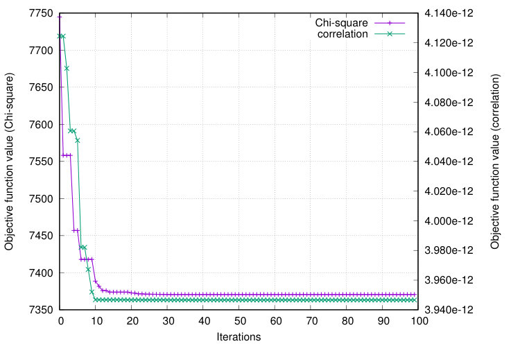 Figure 1
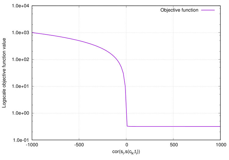 Figure 2
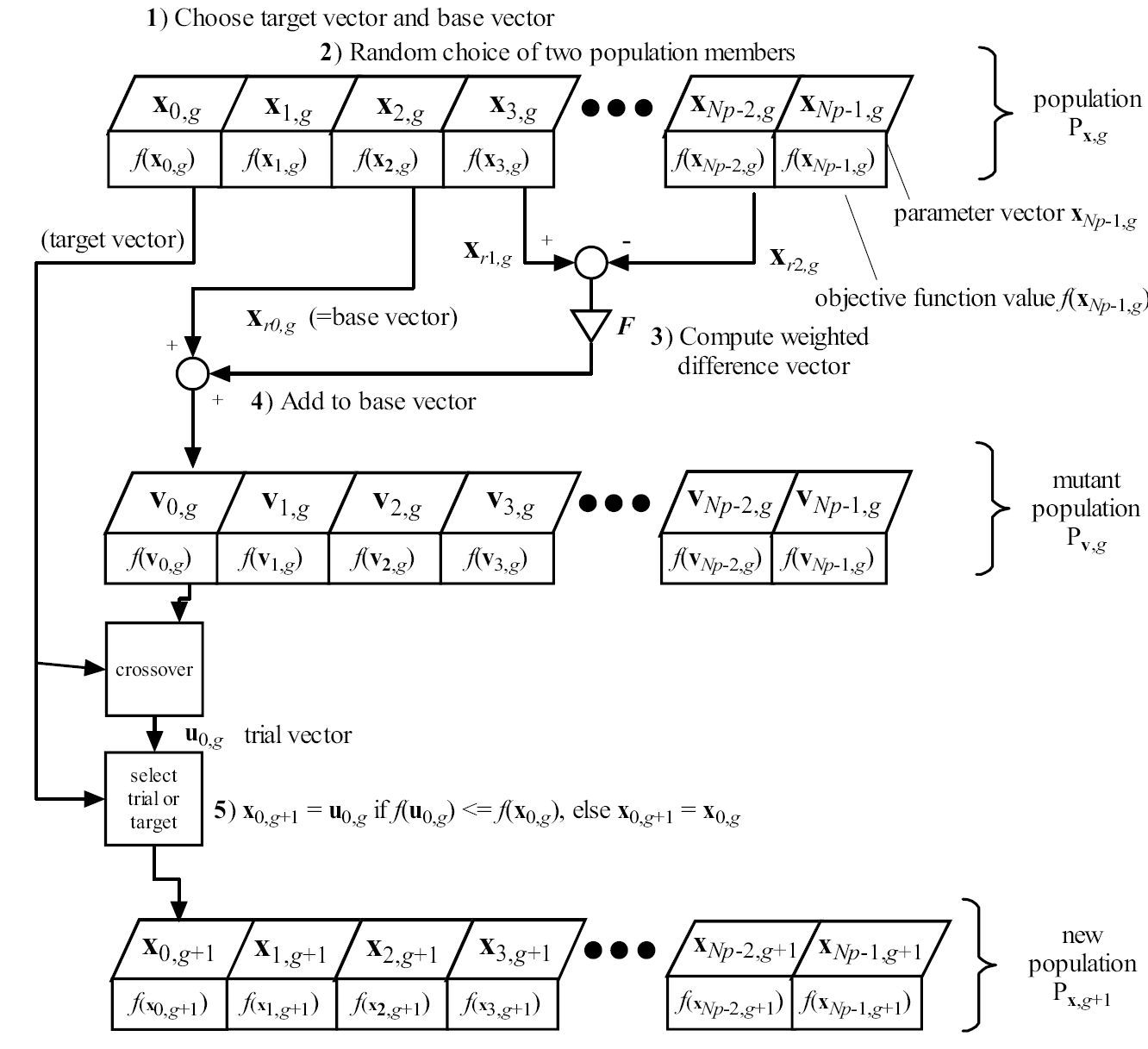 Figure 3
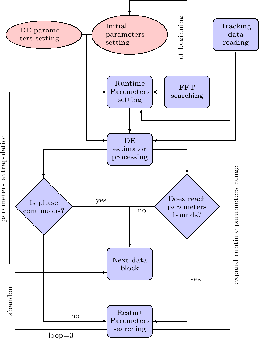 Figure 4
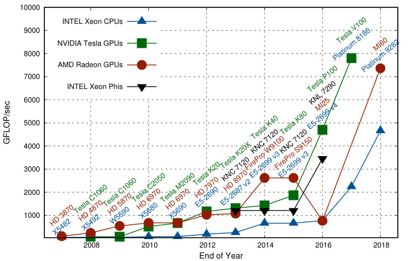 Figure 5
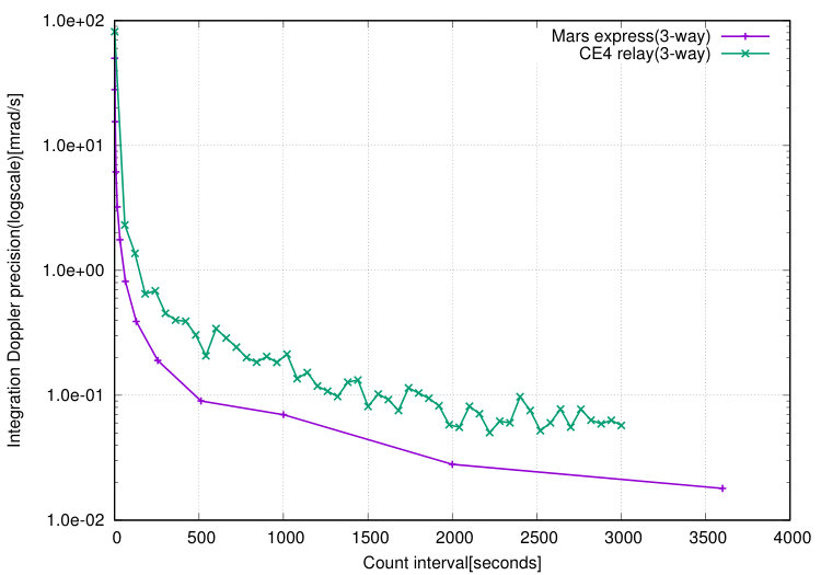 Figure 6
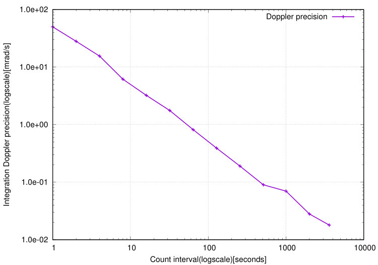 Figure 7
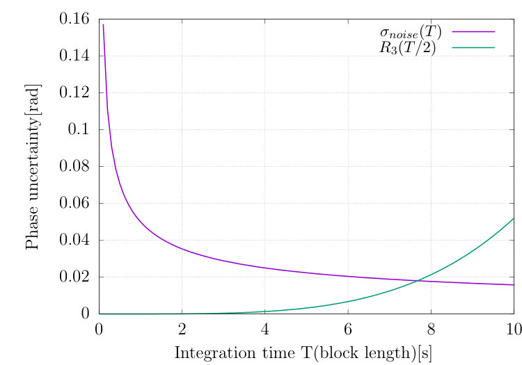 Figure 8
| data volume [Mbit] | GTX580 (GPU) [ms] | OpenMP (CPU) [ms] | VML (CPU) [ms] |
|---|---|---|---|
| 1 | 0.2 | 0.5 | 0.7 |
| 2 | 0.3 | 0.6 | 1.6 |
| 4 | 0.3 | 2.2 | 3.5 |
| 8 | 0.5 | 6.5 | 7.8 |
| 16 | 0.9 | 13.4 | 13.3 |
| 32 | 1.7 | 25.2 | 25.2 |
| 64 | 3.3 | 48.6 | 50.2 |
| 128 | 6.4 | 68.6 | 100.7 |
| 256 | 12.6 | 107.3 | 201.2 |
| manipulation | time consumed |
|---|---|
| Array initialization | 0.039ms |
| Elements square of array | 0.015ms |
| Array linear algebra operation | 0.017ms |
| Array trigonometric operation | 0.016ms |
| Array summation | 0.118ms |
| Total timea | 0.205ms |
| output signal | bandwidth/sampling | quantization |
|
||
|---|---|---|---|---|---|
| narrow band | 16 KHz/32KHz | 8 | 256,000 | ||
| 16 | 512,000 | ||||
| 25 KHz/50KHz | 8 | 400,000 | |||
| 16 | 800,000 | ||||
| 50 KHz/100KHz | 8 | 800,000 | |||
| 16 | 1600,000 | ||||
| 100 KHz/200KHz | 8 | 1600,000 | |||
| 16 | 3200,000 | ||||
| wide band | 1 MHz/2MHz | 1,2,4,8 | 16,000,000 | ||
| 2 MHz/4MHz | 1,2,4,8 | 32,000,000 | |||
| 4 MHz/8MHz | 1,2,4 | 32,000,000 | |||
| 8 MHz/16MHz | 1,2 | 32,000,000 |
| item | Meaning | value |
| dimension of problem | 6 | |
| XCmina | The lower bound of parameters | * |
| XCmana | The upper bound of parameters | * |
| VTR | The expected fitness value of objective function | 0 |
| itermax | The maximum number of iterations | 200 |
| Mutation scaling factor | 0.5 | |
| Crossover factor | 0.85 | |
| strategy | The strategy of the mutation operations | 3—6 |
Peer Reviews
No public reviews on file for this paper yet. If you reviewed it on a platform where reviews are public (OpenReview, ICLR, NeurIPS, ICML), you can paste yours below so the community can read it here.
Videos
No videos yet. Explain this paper in a talk, walkthrough, or lecture? Add one.
Taxonomy
TopicsAstronomical Observations and Instrumentation · Planetary Science and Exploration · Inertial Sensor and Navigation
The GPU-based Phase Tracking method
for Planetary Radio Science applications111This work has been supported by the National Natural Science Foundation of China, the Astronomical Joint Program (U1531104).
Nianchuan Jian
Dmitry Mikushin
Jianguo Yan
Jean-Pierre Barriot
Yajun Wu
Shanghai Astronomical Observatory, Chinese Academy of Science, Shanghai 200030, China
Applied Parallel Computing LLC, Switzerland
State Key Laboratory of Information Engineering in Surveying, Mapping and Remote Sensing,Wuhan University, Wuhan, 430070, China
University of French Polynesia, Geodesy Observatory of Tahiti, Laboratoire GEPASUD, BP 6570, 98702 Faaa airport, Tahiti, French Polynesia
Abstract
This paper introduces a phase tracking method for planetary radio science research with computational algorithm implemented fo r NVIDIA GPUs. In contrast to the phase-locked loop (PPL) phase counting method used in traditional Doppler data processing, this method fits the tracking data signal into the shape expressed by the Taylor polynomial with optimal phase and amplitude coefficients. The Differential Evolution (DE) algorithm is employed for polynomial fitting. In order to cope with high computational intensity of the proposed phase tracking method, the graphics processing units (GPUs) are employed. As a result, the method estimates the instantaneous phase, frequency, derivative of frequency (line-of-sight acceleration) and the total count phase of different integration scales. This data can be further used in planetary radio science research to analyze the planetary occultation and gravitational fields. The method has been tested on MEX (Mars Express, ESA) and Chang’E 4 relay satellite (China) tracking data. In a real experiment with 400K data block size and 80,000 DE solver objective function evaluations we were able to acheive the target convergence threshold in 6.5 seconds and do real-time processing on NVIDIA GTX580 and 2 NVIDIA K80 GPUs, respectively. The precision of integral Doppler (60s) is 2 mrad/s and 4 mrad/s for MEX(3-way) and Chang’E 4 relay satellite(3-way) respectively.
keywords:
Phase tracking, Doppler data processing, Radio sciences, GPU, CUDA
1 Introduction
In deep space exploration missions, radio measurements are often used to study natural phenomena of solar system such as mass and gravity of planets, media around planets and internal structure of planets, etc. This type of research is generally called radio science [Asmar and Renzetti, 1993]. Physical parameters of electromagnetic signal, which links station and spacecraft will be changing during its propagation due to the relative motion of spacecraft and station, influence of medias and the different gravitational potential at the position of spacecraft and station. Physical parameters include phase, frequency, amplitude and polarization. The variation of these parameters allows to estimate the atmospheric and ionospheric structure of planets, solar corona, planetary gravitational fields, shapes, mass, planetary rings and ephemerides of planets. Furthermore, parameters variation allows to verify the theory of general relativity and gravitational waves detection and gravitational red shift [Asmar and Renzetti, 1993; Asmar et al., 2009]. In planetary atmospheric and ionospheric structure studies, the parameters of interest are instantaneous amplitude, phase and frequency. For planetary gravity, ephemerides and the theory of general relativity, the parameters of interest are the integral Doppler or the total count phase. All these parameters can be retrieved through high-precision Doppler measurements.
Since the late 1960s, the Jet Propulsion Laboratory (JPL) has been conducting radio science research in early deep space explorations. Remarkable results have been achieved in the course of 50 years: the high-precision gravity field of Moon and Mars have been determined by Doppler tracking [Lorell and Sjogren, 1968; Konopliv et al., 1998, 2006; Lemoine et al., 2001]; the atmospheric component and ionospheric models of Mars and Venus have been studied from the radio science tracking data. These achievements form the basis of further deep space explorations of human being.
1.1 Planetary radio science hardware
The radio science research is supported by the NASA Deep Space Network (DSN) located at Goldstone (USA), Madrid (Spain) and Canberra (Australia). The DSN is equipped with large antennas (26, 34, and 70 meters) [Asmar and Renzetti, 1993], radio receiver and Doppler processor. The fifth generation of JPL Doppler processors was designed in the form of the the so-called “block series”. The block series are mainly used in precise orbit determination, planetary gravity recovery and general relativity research with close-loop tracking model. The open-loop tracking model receivers have been developed and applied in 1990s’ space missions, such as RSR (radio science receiver) by JPL [Sniffin, 2005] and IFMS (Intermediate Frequency Modulation System) by ESA [Pätzold et al., 2004]. The open tracking model is mainly used in atmospheric and ionospheric studies. Recently, some attempts have been made to apply the open tracking model to the planetary gravity research [Highsmith, 2002].
In Doppler data processing, the amount of computations is large and requires high-performance analysis. The Application Specific Integrated Circuit (ASIC) technology is employed in design of traditional Doppler extractors to compute the phase accumulation (also called phase counting) [Aung et al., 1994]. Nowadays, the general-purpose computing devices also offer enough performance to be used in Doppler data processing software, e.g. the Universal Software Radio Peripheral (USRP) based on GNU Radio222https://www.gnuradio.org/. The USRP can process Doppler data using the FFT-based methods [Løfaldli and Birkeland, 2016].
This paper introduces a new phase tracking method, which employs graphic processing units (GPUs) to compute phase, frequency and frequency derivative of tracking data. The new algorithm fits Taylor polynomial series expanded at data block center to signal existing in the baseband data block333The data block is usually 2 seconds and sampling is 200KHz.. The method calculates the analytical form of phase expression in the neighborhood of the data block center and the amplitude with slope of signal. The amount of baseband fitting computations is large and is offloaded onto GPUs. We show that real-time data processing can be acheived by using two NVIDIA Tesla K80 GPUs. The fitting is performed using Differential Evolution (DE) algorithm [Storn, 1995] – a well-known robust method for global optimization problems. From the analytical form of phase we can further deduce the frequency, derivative of frequency (line-of-sight acceleration) and the integral phase (total count phase) of different time scales [Moyer, 2005]. This data can be used in planetary radio science research to analyze planetary occultation and gravitational fields.
The proposed method has three main advantages over existing hardware and software Doppler processing solutions. Firstly, through the adjustment of the polynomial order and data block length, the analytical form of phase (frequency) will have the phase noise level precision of 444The truncated error is equal to by adjusting. For details please refer to the error analysis below. ( is the data length) along the whole block length. In particular, the method will be more accurate in Doppler processing with high sampling rates (100Hz), required in planetary occultation research. Secondly, the method can resolve the frequency derivative with precision of , directly reflecting the line-of-sight acceleration of the spacecraft relatively to the station (see C). Through the frequency derivative we can solve some further dynamic parameters by means of least square fitting. Thirdly, GPUs are less expensive and easier for software development, compared to traditional ASIC-based Doppler processing equipment.
1.2 Differential evolution algorithm
Doppler data block fitting is a computationally expensive problem, as each objective function evaluation is an integration of time series. Fortunately, the integration can be easily parallelized. Moreover, additional degree of parallelism may be offered by certain kinds of optimization algorithms, such as Differential Evolution (DE). Our numerical results showed that a single objective function evaluation already saturates the compute power of a modern GPU. Therefore, a parallel DE could be performed on multiple GPUs, but we leave this topic out for a separate project.
The DE is a robust global optimization method widely used in various fields to solve multidimensional problems [Price et al., 2006]. The DE algorithm originates from genetic annealing algorithm first described by Price et al. [Price et al., 1994]. The DE algorithm proved itself by winning the International Contest on Evolutionary Optimization (ICEO) twice in 1996 and 1997 [Storn and Price, 1996; Price, 1997].
In DE, the initial population is randomly chosen within the parameter space, and the child parameters vectors are iteratively derived from their parents through the “mutation” procedure, depending on the objective function response (Fig. 1). The mutation is followed by the “crossover“ path selection. In order to escape from local minima, DE introduces a weighting factor. The iterative process continues until the fitfulment of the convergence criteria.
1.3 GPGPU computing
The Graphics Processing Unit (GPU) is a specialized processor originally designed specifically for accelerating video output with complex 3D scenes in games, CADs and visual effects. In order to optimize the speed of positioning and texturing of complex geometries (which involves interpolation), the GPUs have become rich in floating-point compute throughput. Furthermore, the GPU architecture has developed a massive parallelism as a fastest approach to process millions of independent triangles. In early 2000’s, enthusiasts already turned their interest towards general-purpose computations on GPUs (GPGPU) for science and research. However, the GPU programming frameworks of that time (such as GLSL shading language) implied mandatory video output, and did not offer some important features, such as fast shared memory. The GPGPU market has been revolutionized by NVIDIA Corporation in 2007 with the release of GeForce 8 consumer graphic cards with both traditional video processing and compute-only GPGPU pipelines. The GPGPU functionality has become widely available to users through the CUDA v1.0 software development kit [Nvidia, 2010]. Also, NVIDIA released Tesla C870 - the first compute-dedicated graphics card for data centers. Although early GPUs did not offer double-precision computations support, their single-precision performance was a lot higher than on CPUs of the same generaton. During over a decade, NVIDIA GPU technology has seen multiple architectural updates (Tesla, Fermi, Kepler, Maxwell, Volta). The latest NVIDIA Tesla V100 GPU has double-precision peak compute throughput of 7.8 TFLOPS [Rupp, 2013] (see Fig. 2). The CUDA toolkit and GPGPU ecosystem nowadays has grown into a large set of free de-facto standard libraries and frameworks for different purposes: linear algebra (CUBLAS, CUSPARSE), FFT (CUFFT), big data (Thrust), machine learning (TensorFlow), etc.
In our phase tracking method, DE algorithm is employed for solving multidimensional optimization problem. The DE algorithm requires thousands of objective function evaluations, each integrating several dozen points of time series. Along with the basic double precision floating-point multiply-add, the computation of objective function invloves trigonometric operations. Given that the objective function integration is computationally expensive and parallelizable, it becomes an ideal candidate for GPU processing. We offload this part to the GPU by using the Thrust C++ framework [Hoberock and Bell, 2010].
Table 1 compares the time to solution on NVIDIA GTX 580 GPU and 2 Intel E5-2620v2 CPU (which have peak double precision performance of 196 and 60 GFLOPs, respectively). Two implementations have been evaluated on CPU: OpenMP and Intel VML (Vector Math library). The GPU is shown to give about 2 speedup against CPU for a small dataset (below 2M). The speedup improves significantly for larger datasets and reaches 9 for 256M. Furthermore, the OpenMP implementation is faster than VML. Table 2 shows the GPU performance of a single objective function processing steps corresponding to Eq. 2 for 1M dataset.
In a real experiment, the data block size is about 400K (0.082ms on GTX580) and is evaluated by the DE solver 80,000 times to reach the convergence threshold (totals 6.5s on GTX580). Furthermore, by replacing GTX580 with 2 NVIDIA K80s (3.6 TFLOPs peak) we were able to acheive real-time processing.
2 Receiver and signal model
2.1 Receiver overview
The Planetary Radio Science Receiver (PSRS) has been developed under the contract between Shanghai Astronomical Observatory and Southeast University of China and started operation in 2008. The design of PSRS is similar to the RSR receiver framework by JPL [Sniffin, 2005] with 70MHz IF signal input. PSRS has two output channels: the first channel is a narrow band signal recorded on a hard drive after two-stage down conversion from the IF signal; the second channel is a hardware Doppler output after one-stage down conversion. Table 3 shows the available PRSR data recording modes.
In addition to the PSRS receiver, we also use the CDAS(Chinese VLBI Data Acquisition System) receiving device developed by the Shanghai Observatory in the Change’E series missions.
2.2 Signal model and objective function
The first PSRS channel recordered on hard disk has phase errors of various physical origins. The continuous data stream is processed in segments or blocks of length (the value of T is related to the motion of the spacecraft, and is usually set to 2 seconds). If the relative timestamp in the center of the data block has the phase zero, then the whole block can be expanded by a finite Taylor polynomial within the interval [-T/2,T/2]:
[TABLE]
Here is the order of Taylor polynomial which is also related to the motion of the spacecraft. In most of the cases meets the truncation error requirements when block length is set to seconds. Generally, the truncation error is set to the phase noise, which will be discussed later. With the Taylor polynomial phase expression, the radio signal in the data block can be expressed as:
[TABLE]
Here, are the coefficients of Taylor polynomial:
[TABLE]
The coefficients and are signal amplitude parameters. Moreover, is the slope of amplitude and it can be ignored when amplitude change is small with data length below 10 seconds.
Differential Evolution (DE) algorithm minimizes the objective function, which is generally non-negative. From Eq. 2 we construct two types of objective functions. The first one is the classical function and the second one is based on the correlation function:
[TABLE]
[TABLE]
In Eq. 4, is the weighting factor that is relative to the standard deviation of signal influenced by physical environment. Influence is equal to every data point. So weighting factor can be set to 1. The optimal coefficients are to be determined. The is the signal model constructed in Eq. 2, and is the quantized signal value. The and objective functions shall converge to the sum of noise power, and to , respectively. In Eq. 5 the signal model is slightly changed, such that the amplitude of signal is constant; otherwise, the objective function becomes divergent:
[TABLE]
Here, is the average amplitude of signal. Fig. 3 shows the relation between and . The figure also shows that the convergence is very fast when the correlation coefficient is close to zero. Fig. 4 compares the convergence rate of two objective functions types.
The data used for comparison is the real Mars Express (MEX) tracking data with the baseband sampling of 200KHz. For the convenience of display, the correlation objective function value is subtracted a constant of 0.31830988618. The figure shows the is faster to converge than , and takes only 10 times iterations. On the other hand, requires 25 times iterations. Moreover, the computational difficulty of one evaluation is only 60% of function. In total, the takes 75% less time to compute a data block, compared to . Although the is faster than , it cannot handle larger block sizes, which have significant signal amplitude change.
3 Data processing and error analysis
3.1 Data processing
This subsection will introduce the parameters setting for DE algorithm, phase continuity checking and process flow in real data processing.
3.1.1 Determination of parameters range
Determination range of parameters to be solved are required when calling DE algorithm which must cover the true value of parameters. Because DE algorithm is a kind of global optimisation, generally speaking range of parameters can be enlarged widely enough to cover the true value of parameters. But this strategy will cause huge amount of computation. So properly determine the initial value and range of parameters is necessary for high efficient computation. The range Determination includes initial range setting and running time range setting. Following content of this subsection will discuss these two kind of range settings based on function model mentioned in Eq. 4.
Determination of proper initial range of parameters needs estimation of parameters. From Eq. 3 we can see that the polynomial coefficients are determined by derivatives of phase at block center. So if we can estimate the derivatives of phase at block center then polynomial coefficients could be properly determined. The detailed estimation process is as follows:
* is the instantaneous phase at block center, range can be set as .* 2. 2.
* is the instantaneous frequency at block center (). It can be determined through FFT computation of a small piece of data extracted from block center. Range of can be setted as *10% of . 3. 3.
* is equal to half of second derivative of phase at block center. So the value of can be estimated by central difference method through three equally spaced frequency values near block center. The frequency value ls calculated as step 2* 4. 4.
* is the 1/6 of third derivative of phase at block center. This term is very small and will not be greater than 10 in all situations. In real data processing initial range of is set to for the sake of insurance.* 5. 5.
* is the amplitude of signal. It can be determined by FFT algorithm done at step 2. Range of can be set as *10% of . 6. 6.
* is the slope of amplitude which relative uncertainty is big when block length is not longer enough. For the sake of insurance it’s range is set as .*
If there is a forecast orbit of spacecraft derivatives of phase at block center also can be properly estimated from orbit using Eq. 11.
Determination of range of parameters at running time is exactly automatic tracking of the signal. Extrapolation is used in coefficients of Taylor polynomial estimation from th block to th block. The specific running time range estimation of is as follows:
Range of is the same as initial range setting 2. 2.
Value of can be extrapolated from the first-order phase derivative of block (Eq. 1): . So the value is , and range could be set as 555The sign will be decided by software automatically. 3. 3.
Value of can be extrapolated as , that is . Range could be set as 4. 4.
Value of is small and the range can be further narrowed from the result of first time of DE calling. 5. 5.
Range of is 6. 6.
Range of can be fixed as
Range setings by means of extrapolation of and are effective in most situations that is when derivatives of phase is monotonic functions. But when derivatives of phase are not monotonic functions within two blocks the range of parameters will not cover the true value and parameters searching will failed. This generally happens while the spacecraft crossing the orbital apogee or perigee. The software will automatically restart searching after properly enlarge the range of parameters. Meanwhile the values of and are random distribution when data length is not long enough(that is the signal to noise ratio is not big enough)( A)
3.1.2 The DE algorithm control parameters setting
The DE algorithm runs under a set of control parameters. Table 4 gives the explanation of these control parameters and values set for running.
There are six kind of mutation operations strategies in the DE algorithm which affect the solution robustness and computation speed[Price et al., 2006]. Among these strategies the third is the best choice for objective function Eq. 4 and the sixth for Eq. 5. Two type of stop condition are generally used for parameters searching. The first is fixing the iteration number when proper parameters range can be determined at running time. The second is setting the threshold of change of objective function or parameters. In practical applications parameters and objective function sometimes remain the same in several iterations because of the characteristics of genetic algorithms. So the first type of stop condition is used in real data processing.
3.1.3 Phase continuity checking
A natural method to judge weather solution is perfect is to check the continuity of instantaneous phase and frequency at the bound of two adjacent data block. Using Eq. 1 we can get the expression of phase and frequency:
[TABLE]
Phase and frequency at the bound of two adjacent data block (n and n+1) are:
[TABLE]
Checking weather the values of and are equal to and within the threshold of noise we can confirm the correctness of parameters result from DE algorithm. A real data processing example of MEX shows continuity of phase and frequency in A. The noise of phase is about (1 , 1 second integration) in MEX tracking. So the continuity of phase can be confirmed.
3.1.4 Data process flow
The software reads the initial parameters range and the DE algorithm controls parameters from control file and runs automatically without manual intervention. Fig. 5 gives the process flow.
In radio measurement there exist some accidental factors that cause phase distortion and iterations divergence. In this situation the software will automatically adjust parameters range and try to search again. The data block will be abandoned after three attempts.
3.2 Error analysis
There are three kind of errors in data process. The first error is the truncation error in phase calculation which is also called remainder of Taylor polynomial. The second error is random errors in tracking data. The third is system error caused by equipments and medias along the signal path. Remainder of Taylor polynomial is relative to the block length and polynomial order. Random errors come from thermal noise of signal beacon, receiver and medias along signal path. System error can be eliminated by construction of error models in high level data process which is no in the scope of this paper and will not be discussed.
3.2.1 Remainder of Taylor polynomial
Remainder of Taylor polynomial has several expression forms. Lagrange error bound is usually used for error analysis. Lagrange error bound of Eq. 1 can be written as:
[TABLE]
is a point within [0,t]. The max error within data block is generally at the block border. Remainder at block border is:
[TABLE]
Here \big{|}\phi^{(n+1)}_{max}\big{|} is maximum absolute value of th derivative of phase within data block. From Eq. 10 we can see the upper bound of remainder is relative to the order of Taylor polynomial , length of data block and the absolute value of maximum th derivative of phase. Generally speaking 666In the following contents of this paper, if not specified, the default value of . can ensure the remainder small enough with which upper bound of \big{|}\phi^{(n+1)}_{max}\big{|} will be (See B). When the block length is not so long(less than 10 seconds) in this situation the upper bound of truncation error of Taylor polynomial is . But in some special cases such as aircraft passing across perigee or flying-by a giant planet amplitude of \big{|}\phi^{(n+1)}_{max}\big{|}|_{n=3} can not be ignored (this term is about while MEX passing across perigee) and is not enough for high precision data processing. In this situation will be work and the upper bound of truncation error could be controlled within . Derivatives of phase can be estimated from the derivatives of line-of-sight velocity using forecast orbit:
[TABLE]
In theory, if there is no effect of thermal noise the truncation error can be controlled very small by adjusting the parameters and . But thermal noise has traits that cannot be eliminated. Excessively reducing the truncation error is futile. So the threshold of truncation error can be set to the thermal noise of phase . Here is integration time for measuring phase noise which is exactly the block length. Pätzold et al. have given a relative expression of
[TABLE]
is standard thermal noise when integration time is equal to 1 second. From the Eq. 12 we can infer that thermal noise can be effectively suppressed by increasing the integration time.
There exists a choice of to balance the truncation error and thermal noise from Eq. 10 and Eq. 12. On the one hand, the remainder and are positively correlated. On the other hand, the thermal noise and are negatively correlated. The length of is worth considering to balance the computation amount and the data process precision. Fig. 6 gives the relationship of truncation error and phase thermal noise relative to block length in MEX tracking case ().
From Fig. 6 we can see that truncation error will be less than phase thermal noise when block length is shorter than 7 seconds. In the actual data processing, to ensure that the truncation error is less than the phase noise and improve the data processing efficiency, the data block length is generally set to 2 seconds.
3.2.2 Random phase noise
Random noise in data will affect the estimation of phase and it can be used as criteria for truncation error as described above. Random noise comes from two sources. The first is the thermal noise of signal source, transponder on board and receiver at station. The second is random interference of solar phase scintillations along signal path. Carrier phase error variance can be expressed as [Sniffin, 2005]:
[TABLE]
Here,
- •
* is contribution to carrier loop phase error variance due to solar phase scintillations*
- •
* is downlink carrier loop signal-to-noise ratio*
- •
* is transponder ratio*
- •
* is one-sided, noise-equivalent, transponder carrier loop bandwidth*
- •
* is one-sided, noise-equivalent, loop bandwidth of downlink carrier loop*
- •
* is uplink carrier power to noise spectral density ratio*
Phase error variance contributed by solar phase scintillations is related to the angle SEP (Sun Earth Probe). This effect is greater when the sun is near the direction of observation. Eq. 14 gives the relation between and SEP [Sniffin, 2005]:
[TABLE]
In Eq. 14 are constants which vary with frequency band. For X band of up and down link .
The typical magnitudes of phase noise for 2/3 way tracking at X band are [Yuen, 2013]:
[TABLE]
Eq. 15 gives the upper bound of phase noise variance for three types of carrier modulation.
4 Applications
Using the Taylor polynomial coefficients estimated by the DE algorithm we can form several kinds of observables including integration Doppler, instantaneous Doppler, total count phase and line-of-sight acceleration.
4.1 Doppler observables
4.1.1 Integration Doppler
Integration Doppler is an important observation type in planetary gravity research. The original definition of integration Doppler is the phase change during an fixed count interval [Moyer, 2005]:
[TABLE]
Here we ignore the bias for the convenience of discussion. is the station time at the end of count interval and is the station time at the beginning of count interval. is the count interval length which is different for different research object. Typical count times have durations of tens of seconds in planetary gravity research while spacecraft orbiting planet. In testing theory of general relativity and gravitational wave searching [Asmar and Renzetti, 1993; Asmar et al., 2009] interval of counting will be few thousand seconds for extremely high Doppler measurement precision during interplanetary cruise.
The typical data block length is 2 seconds and the limitation of data block length is 20 seconds limited by the processing ability of the GPU. We can use phase connection to form the longer integration Doppler observables:
[TABLE]
In Eq. 17 is serial number of block, can be evaluated by phase expression (Eq. 7), is the phase change within count interval which is also a new kind of observation type in planetary science research [Moyer, 2005]. The column 8 of A gives the example of . Uncertainty of Integration Doppler can be expressed as:
[TABLE]
Meaning of the Eq. 18 is the same as Eq. 12. is phase variance of block or the phase discontinuous variance at block border.
Figure 7 shows the precision of integration Doppler with different interval scales in MEX and CE4 data process.
The Doppler precision is about : for MEX with 1 second Integration schale and : for CE4 relay satellite.
4.1.2 Instantaneous Doppler
Instantaneous Doppler is used in planetary occultation research in which high Doppler resolution is required at ingress or egress of radio signal into or out of planetary atmosphere. There are two kinds of approximate approaches to compute instantaneous Doppler. The first is to decrease the count interval [Moyer, 2005] and use integration Doppler to approximate instantaneous Doppler. The second is using short time Fast Fourier Transform (FFT) to compute an average frequency of a short data block [Pätzold and Häusler, 2000]. The Doppler precision of these two approaches will obey Eq. 12 that is times of when Doppler sampling rate is 10 Hz.
Using Eq. 7 we can conveniently calculate instantaneous Doppler at any time tag within data block and the precision is guaranteed by the truncated error which is 0.7 times of . So instantaneous Doppler calculated from Taylor polynomial has higher precision than method of short count interval or method of short time FFT.
4.2 Line-of-sight acceleration observables
From Eq. 11 we can see that derivatives of phase is related with the derivatives of line-sight-of velocity and second derivative of phase can be approximated as function of line-sight-of acceleration:
[TABLE]
A strict and full expansion of Eq. 19 can be found in section C which gives connection between observable of and dynamic state of spacecraft and stations. Combined with a tracking case of MEX magnitude analysis of line-of-sight acceleration is given in which magnitude of line-of-sight acceleration in Newtonian frame is about 1 , cross velocity terms have magnitude of in first order of Eq. 29, and main term of second order of Eq. 29 is about .
Base on the concept of C we give an estimation of the mass and two order of gravity of Phobos [Jian et al., 2019]. The line-of-sight acceleration observable () directly reflects the kinematic state of the spacecraft () and can be used to estimate the dynamic parameters relative to spacecraft() corporation with a reference orbit. It also can be used in process of least square regress combined with traditional Doppler observables to solve parameters.
5 Conclusion
This paper introduces a new phase tracking method for planetary radio science research based on GPGPU (General Purpose Computing on GPU) technology. In addition to Doppler observables used in planetary radio science research the new method also gives the line-of-sight acceleration observable which directly reflects the dynamic state of the spacecraft. Using line-of-sight acceleration we can directly solve the dynamic parameters interested with a reference orbit.
6 Acknowledgments
This work has been supported by the National Natural Science Foundation of China, the Astronomical Joint Program (U1531104). We thank Mr. Gou Wei from Sheshan 25-meter Observatory for assistance in MEX tracking, Prof. Meng Qiao, Chen Congyan and Lu Rongjun of Southeast University of China for advice on Doppler data processing, and Prof. Ping Jinsong of National Observatory of China for helpful conversations.
Appendix A 1
**Phase tracking output example for MEX tracking **
           UTC time             c_0(rad) c_1(rad/s)    c_2(rad/s^2)    c_3      c_4          c_5     total_phase   RSS       data quality index
  (border) 2013-12-28T19:24:38   6.102   146782.529
block1(center) 2013-12-28T19:24:39 5.670 146566.029 -108.151807 0.066 4728.3 6.7 293132.189 3424636.172 1 (border) 2013-12-28T19:24:40 2.563 146349.922 (border) 2013-12-28T19:24:40 2.585 146349.721 block2(center) 2013-12-28T19:24:41 3.319 146133.984 -107.928933 -0.040 4713.0 -18.4 292267.887 3417344.713 1 (border) 2013-12-28T19:24:42 1.824 145918.005 (border) 2013-12-28T19:24:42 1.831 145918.155 block3(center) 2013-12-28T19:24:43 4.412 145702.273 -107.838436 0.068 4721.2 -10.5 291404.683 3425031.927 1 (border) 2013-12-28T19:24:44 4.946 145486.801 2013-12-28T19:24:44 4.933 145486.642 ... 2013-12-28T19:24:45 3.474 145271.151 -107.703009 0.028 4749.4 -2.9 290542.359 3427429.823 1 2013-12-28T19:24:46 0.237 145055.830 2013-12-28T19:24:46 0.238 145055.809 ... 2013-12-28T19:24:47 1.568 144840.493 -107.600678 0.038 4710.2 2.9 289681.063 3423038.571 1 2013-12-28T19:24:48 1.325 144625.406 2013-12-28T19:24:48 1.316 144625.163 2013-12-28T19:24:49 5.865 144410.414 -107.439969 -0.044 4725.1 -35.5 288820.741 3419870.188 1 2013-12-28T19:24:50 2.878 144195.403 2013-12-28T19:24:50 2.893 144195.292 2013-12-28T19:24:51 4.936 143980.762 -107.331095 -0.044 4726.0 -0.9 287961.436 3424449.594 1 2013-12-28T19:24:52 5.946 143765.968 2013-12-28T19:24:52 5.962 143766.015 2013-12-28T19:24:53 5.951 143551.478 -107.244130 0.016 4711.1 -4.7 287102.989 3424489.034 1 2013-12-28T19:24:54 5.081 143337.038 2013-12-28T19:24:54 5.106 143337.164 2013-12-28T19:24:55 3.608 143122.853 -107.113158 0.028 4710.5 -5.7 286245.762 3419445.809 1 2013-12-28T19:24:56 1.512 142908.711 2013-12-28T19:24:56 1.497 142908.715 2013-12-28T19:24:57 5.237 142694.705 -106.952688 0.035 4709.9 2.9 285389.480 3418848.526 1 2013-12-28T19:24:58 2.417 142480.904 2013-12-28T19:24:58 2.437 142480.624 2013-12-28T19:24:59 5.570 142267.018 -106.825240 -0.015 4682.0 6.7 284534.007 3433902.863 1 2013-12-28T19:25:00 2.398 142053.323 ... ...
Here, integration length of total_phase (colum 8 above) is the block length
Appendix B 2
Appendix C 3
**Observation function of second derivative of phase
**
Acronyms:
- •
1 foot mark means uplink station
- •
2 foot mark means satellite
- •
3 foot mark means downlink station
- •
c speed of light in vacuum
- •
coordinate time at position i
- •
position vector of object i in inertia frame
- •
position vector of object j relative to i
- •
velocity vector of object i in inertia frame
- •
velocity vector of object j to i
- •
acceleration vector of object i in inertia frame
- •
frequency transmitted from uplink station
- •
transponder turnaround ratio onboard
- •
frequency received by downlink station
- •
atomic clock of downlink station
- •
distance from position i to j
- •
deviation of distance from position i to j
- •
Newtown gravitation at position i
- •
velocity magnitude of object i relative to Sun
- •
SSB Solar System Barycenter
- •
Lagrangian constant of astronomy
C.0.1 2/3 way tracking model
Theodore D. Moyer gives a precise formula accurate to describing the sky frequency received by downlink station in 2/3-way tracking models [Moyer, 1971].
[TABLE]
Using above equation the derivative of to can be written as( terms):
[TABLE]
Expansion of right side of above equation:
[TABLE]
Expansion of partial derivatives of velocity to coordinate time:
[TABLE]
Relation between coordinate time and station time [Moyer, 1971]:
[TABLE]
Relation of coordinate time of different objects and definitions of relative velocity:
[TABLE]
By substituting Eq. 21, 22, 23, 24, 25 into Eq. 20 we can get the first order of expansion for the derivative of to .
Expansion of terms of Eq. 20777The last two terms are very small() and will be ignored.:
[TABLE]
Some terms have been expanded in Eq. 22 and 25 and remains can be expanded as:
[TABLE]
Derivatives of different time scales can be found in Eq. 24 and 25. Remain terms of Eq. 27 can be expanded as:
[TABLE]
By substituting Eq. 24, 25, 27, 29 into Eq. 26 we can get the expansion of terms of Eq. 20
Formal the second derivative of phase can be written as:
[TABLE]
Here scale of station time is the same as time tag of data block. So the phase derivatives are equal to each other:
[TABLE]
C.0.2 Magnitude estimation of with case of MEX mission
Considering a common 3-way tracking of MEX with uplink station of New Norcia located at Australia and downlink station of Sheshan located at China:
- •
Distance from station to MEX: Km
- •
Distance between stations: Km
- •
Velocity of station relative to SSB: Km/s
- •
Velocity of MEX relative to SSB Km/s
Considering that the distance between station and spacecraft is much larger than the distance between stations, the following relationship is defined and established.
[TABLE]
Here, is unit vector of opposite direction of line-of-sight.
**First order of Eq. 29
**By ignoring the influence of gravitation on time scale derivative(Eq. 24) first order of Eq. 29 can be simplified as:
[TABLE]
In the equation Amplitude of and in the frame of SSB is about due to Earth rotation and amplitude of (MEX) is about due to orbit motion. are cross velocity terms with dimension of acceleration and with amplitude of :
[TABLE]
Definition of factor(amplitude is about ):
[TABLE]
If we ignore the contributions of and , Eq. 32 can be further simplified as(in Newtonian frame):
[TABLE]
Here we can see that in Newton frame the second derivative of phase could be approximated as function of line-of-sight acceleration of and with error of .
**Second order of Eq. 29
**The second order888Here is treated as constant. of Eq. 29 can be simplified to order of :
[TABLE]
Here, terms are defined in Eq. 33 and new definitions of are(with amplitude of ):
[TABLE]
The main term of Eq. 36 approximates to .
The reference list from the paper itself. Each links out to its DOI / PubMed record.
- 1Asmar and Renzetti [1993] S. Asmar, N. Renzetti, The deep space network as an instrument for radio science research, NASA STI/Recon Technical Report N 95 (1993) 21456.
- 2Asmar et al. [2009] S. W. Asmar, K. Aksnes, R. Ambrosini, A. Anabtawi, J. D. Anderson, J. W. Armstrong, D. Atkinson, J.-P. Barriot, B. Bertotti, B. G. Bills, et al., Planetary radio science: Investigations of interiors, surfaces, atmospheres, rings, and environments, A White Paper (2009).
- 3Lorell and Sjogren [1968] J. Lorell, W. Sjogren, Lunar gravity: Preliminary estimates from lunar orbiter, Science 159 (1968) 625–627.
- 4Konopliv et al. [1998] A. Konopliv, A. Binder, L. Hood, A. Kucinskas, W. Sjogren, J. Williams, Improved gravity field of the moon from lunar prospector, Science 281 (1998) 1476–1480.
- 5Konopliv et al. [2006] A. S. Konopliv, C. F. Yoder, E. M. Standish, D.-N. Yuan, W. L. Sjogren, A global solution for the mars static and seasonal gravity, mars orientation, phobos and deimos masses, and mars ephemeris, Icarus 182 (2006) 23–50.
- 6Lemoine et al. [2001] F. G. Lemoine, D. E. Smith, D. D. Rowlands, M. Zuber, G. Neumann, D. Chinn, D. Pavlis, An improved solution of the gravity field of mars (gmm-2b) from mars global surveyor, Journal of Geophysical Research: Planets 106 (2001) 23359–23376.
- 7Sniffin [2005] R. Sniffin, DSMS Telecommunications Link Design Handbook, Technical Report, JPL/NASA Technical Report, 2005.
- 8Pätzold et al. [2004] M. Pätzold, F. Neubauer, L. Carone, A. Hagermann, C. Stanzel, B. Häusler, S. Remus, J. Selle, D. Hagl, D. Hinson, et al., Mars: Mars express orbiter radio science, in: Mars Express: The Scientific Payload, volume 1240, pp. 141–163.