Bandgap-Assisted Quantum Control of Topological Edge States in a Cavity
Wei Nie, Yu-xi Liu

TL;DR
This paper proposes an optical control method for topological quantum states in a superconducting qubit array coupled to a cavity, revealing how topological bandgaps influence light-matter interactions and enable quantum state engineering.
Contribution
It introduces a novel cavity-qubit coupling scheme to observe topological phase transitions and demonstrates the protective role of bandgaps in quantum interference and photon transport.
Findings
Topological bandgap protects edge state Rabi splitting from bulk states.
Cavity-induced coupling between edge states dominates in the dispersive regime.
Quantum interference enables single-photon transport across boundaries.
Abstract
Quantum matter with exotic topological order has potential applications in quantum computation. However, in present experiments, the manipulations on topological states are still challenging. We here propose an architecture for optical control of topological matter. We consider a topological superconducting qubit array with Su-Schrieffer-Heeger (SSH) Hamiltonian which couples to a microwave cavity. Based on parity properties of the topological qubit array, we propose an optical spectroscopy method to observe topological phase transition, i.e., edge-to-bulk transition. This new method can be achieved by designing cavity-qubit couplings. A main purpose of this work is to understand how topological phase transition affects light-matter interaction. We find that topological bandgap plays an essential role on this issue. In topological phase, the resonant vacuum Rabi splitting of degenerate…
Click any figure to enlarge with its caption.
 Figure 1
 Figure 2
 Figure 3
 Figure 4
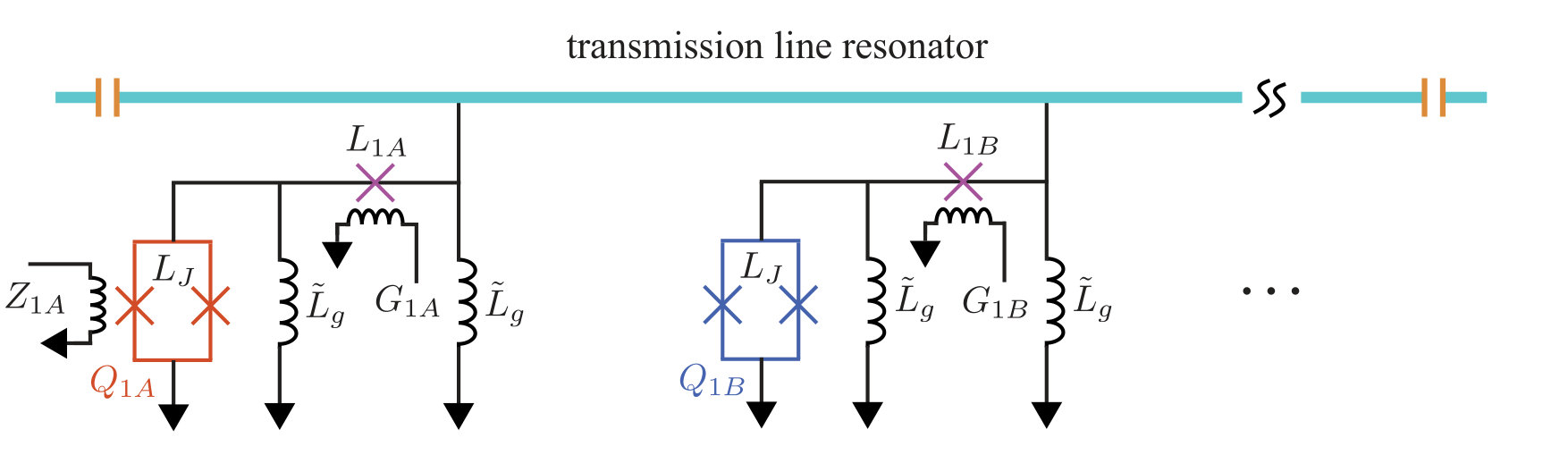 Figure 5
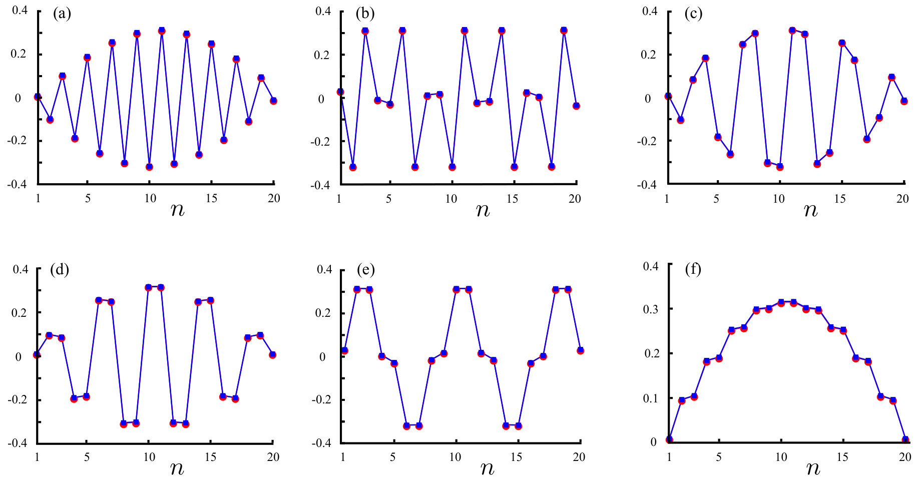 Figure 6
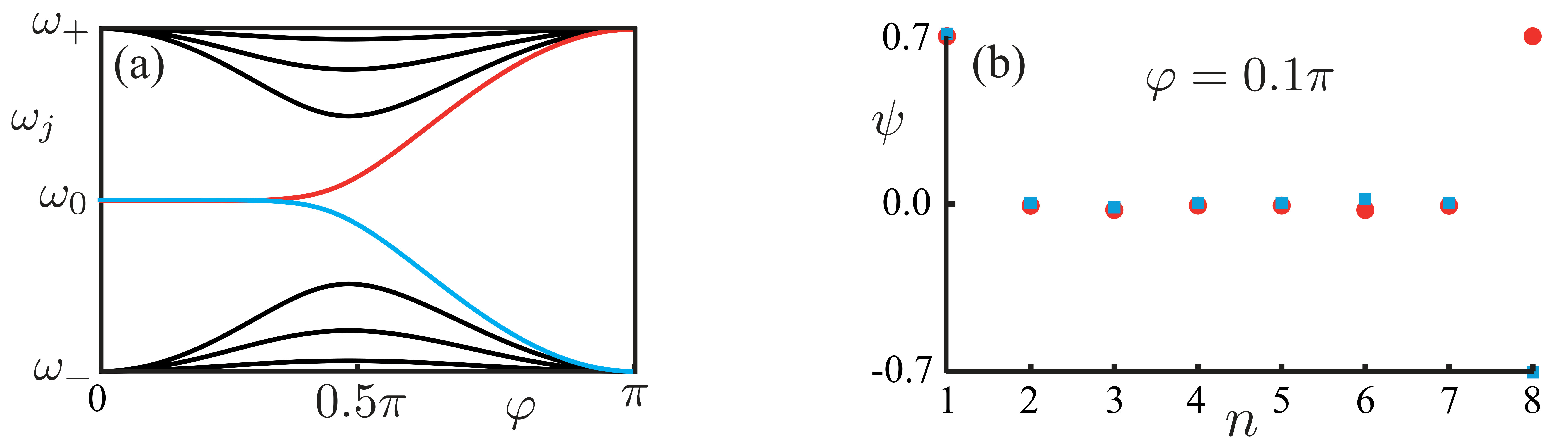 Figure 7
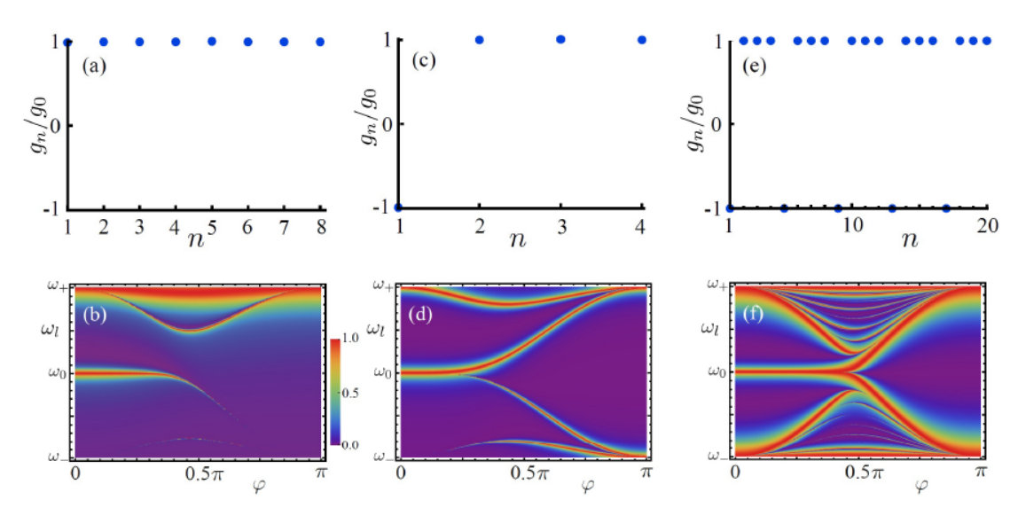 Figure 8
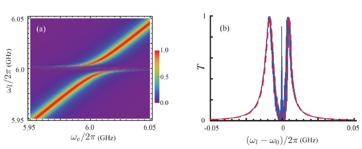 Figure 9
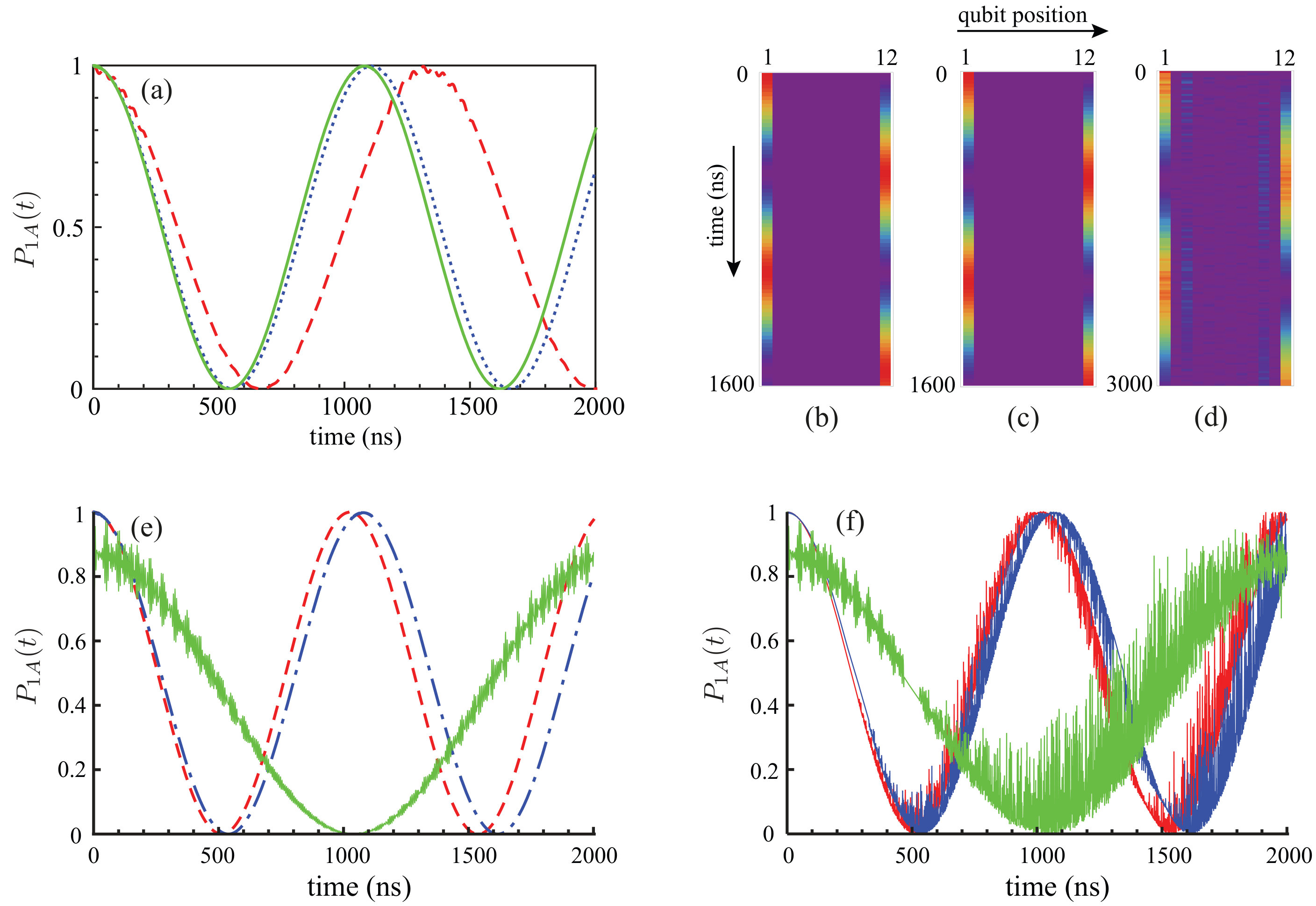 Figure 10
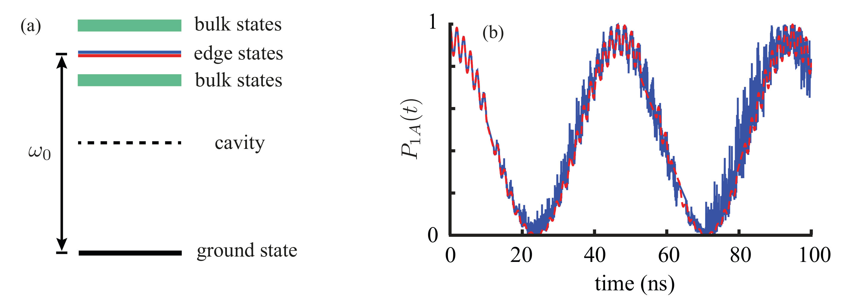 Figure 11
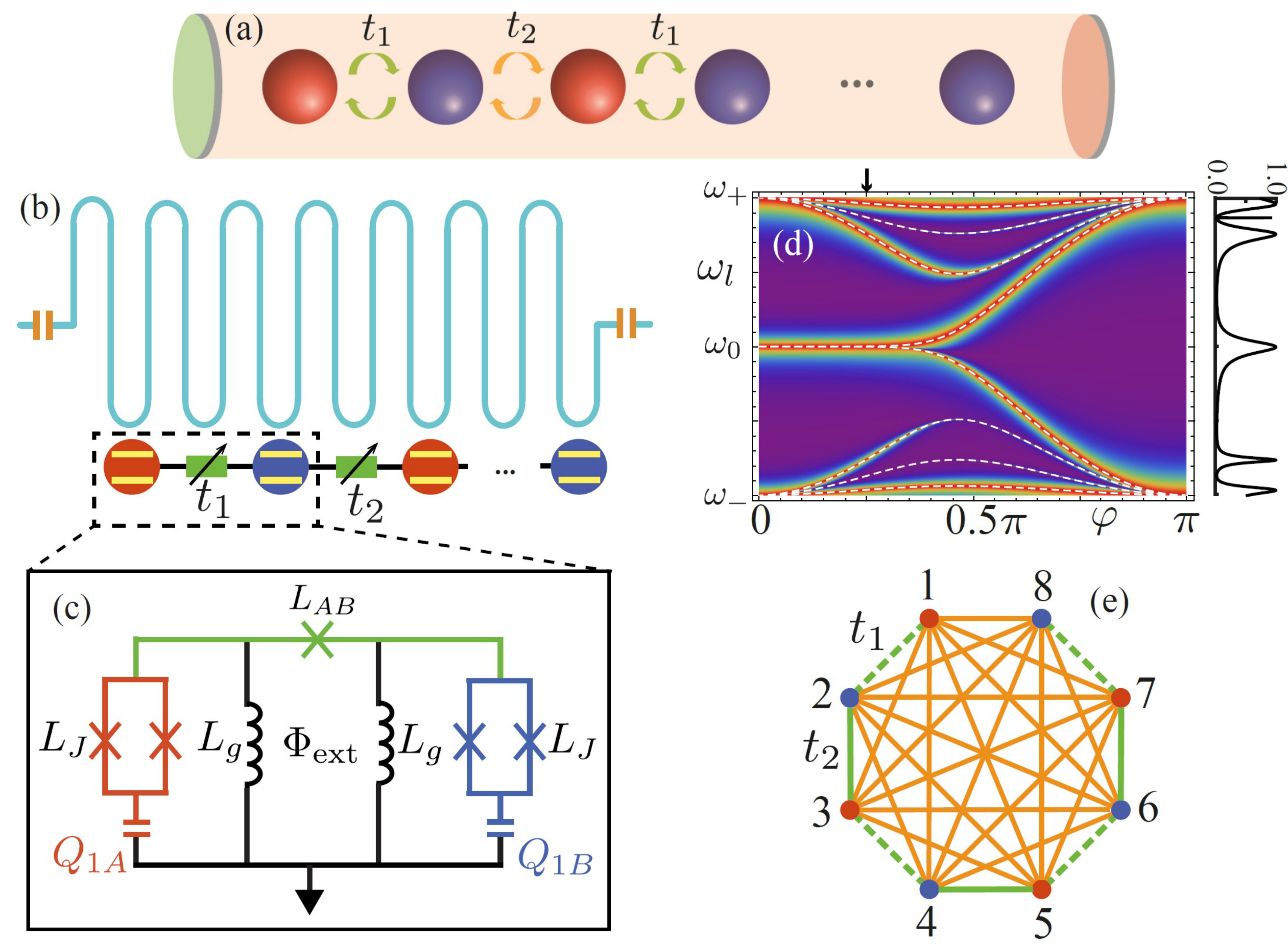 Figure 1
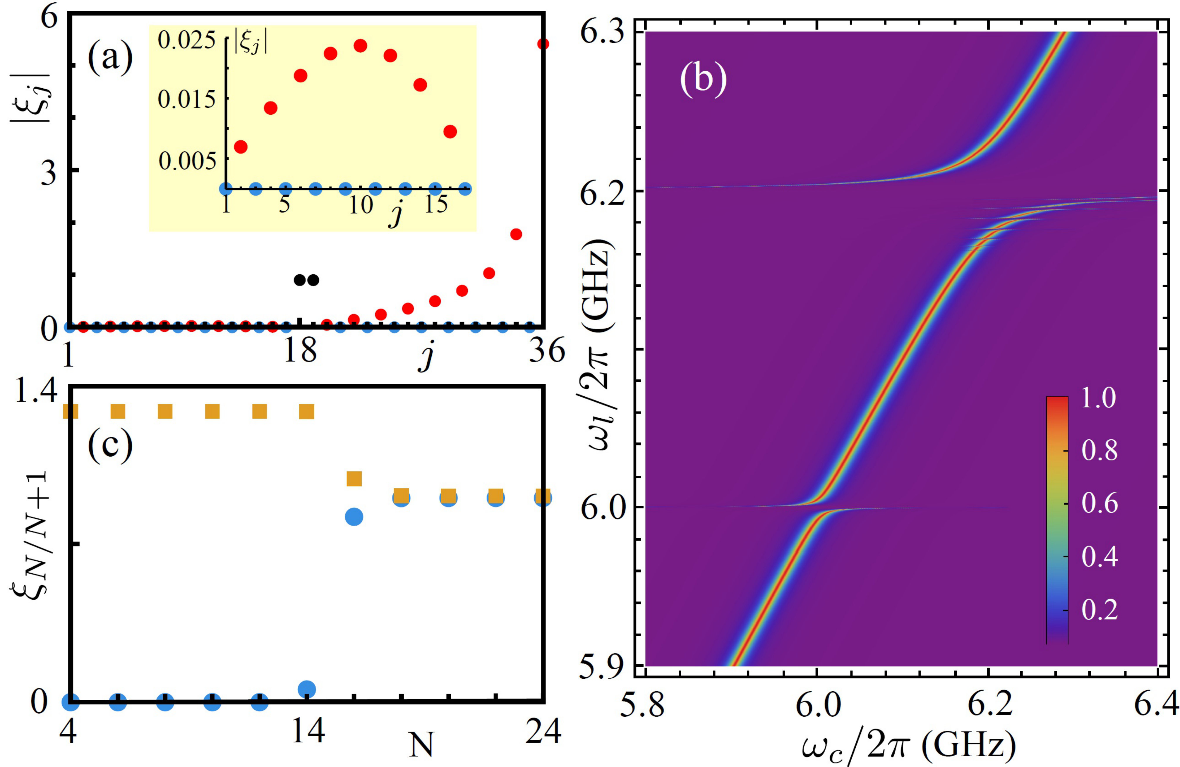 Figure 2
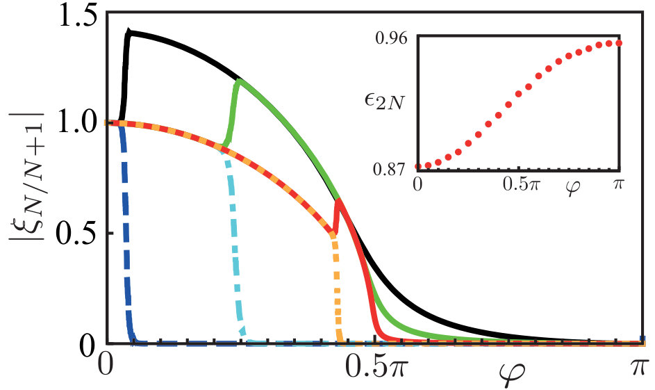 Figure 3
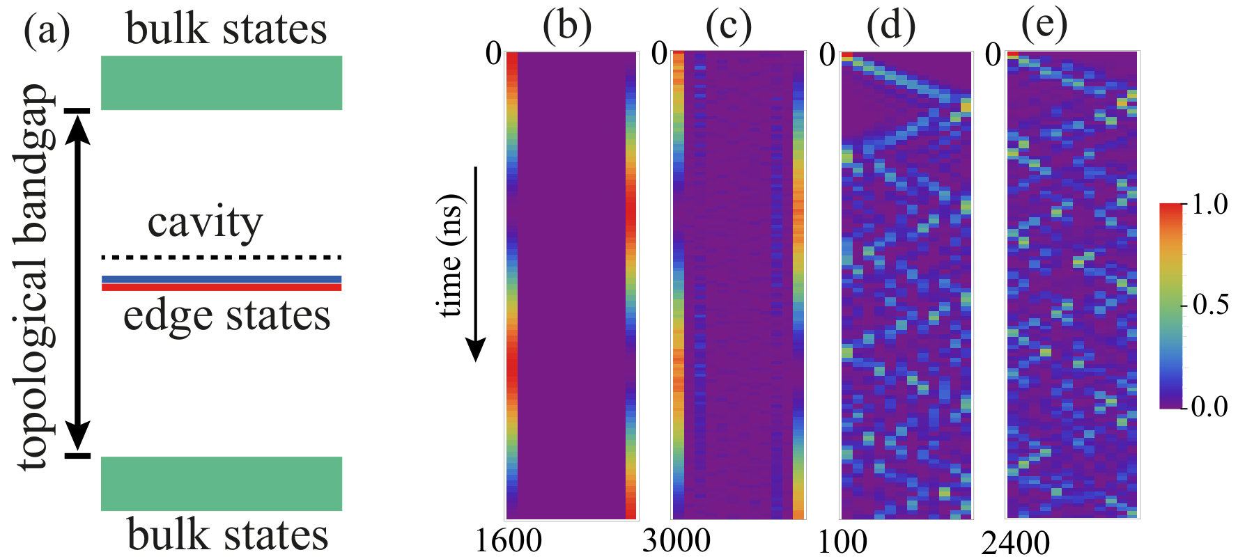 Figure 4
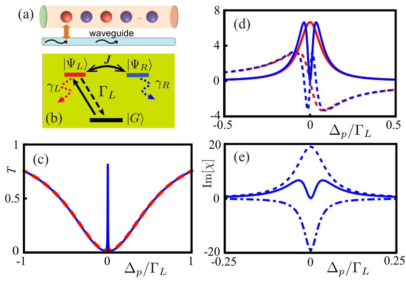 Figure 5
Peer Reviews
No public reviews on file for this paper yet. If you reviewed it on a platform where reviews are public (OpenReview, ICLR, NeurIPS, ICML), you can paste yours below so the community can read it here.
Videos
No videos yet. Explain this paper in a talk, walkthrough, or lecture? Add one.
Bandgap-Assisted Quantum Control of Topological Edge States in a Cavity
Wei Nie
Institute of Microelectronics, Tsinghua University, Beijing 100084, China
Yu-xi Liu
Institute of Microelectronics, Tsinghua University, Beijing 100084, China
Frontier Science Center for Quantum Information, Beijing, China
Abstract
Quantum matter with exotic topological order has potential applications in quantum computation. However, in present experiments, the manipulations on topological states are still challenging. We here propose an architecture for optical control of topological matter. We consider a topological superconducting qubit array with Su-Schrieffer-Heeger (SSH) Hamiltonian which couples to a microwave cavity. Based on parity properties of the topological qubit array, we propose an optical spectroscopy method to observe topological phase transition, i.e., edge-to-bulk transition. This new method can be achieved by designing cavity-qubit couplings. A main purpose of this work is to understand how topological phase transition affects light-matter interaction. We find that topological bandgap plays an essential role on this issue. In topological phase, the resonant vacuum Rabi splitting of degenerate edge states coupling to the cavity field is protected from those of bulk states by the bandgap. In dispersive regime, the cavity induced coupling between edge states is dominant over couplings between edge and bulk states, due to the topological bandgap. As a result, quantum interference between topological edge states occures and enables single-photon transport through boundaries of the topological qubit array. Our work may pave a way for topological quantum state engineering.
Introduction.—Characterization of topological matter is a crucial issue in condensed matter physics Bansil et al. (2016). A hallmark of topological phases is the existence of topological invariants, e.g., Chern number and Zak phase, defined on energy bands of the systems Thouless et al. (1982); Zak (1989); Xiao et al. (2010). According to edge-bulk correspondence, topological states emerge in the bandgaps and give rise to many novel transport phenomena Law et al. (2009); Fu (2010). Due to their insensitivity to local decoherence, topological states have prospective applications in quantum information processing. In particular, zero-dimensional edge states, e.g., Majorana bound states are candidate to realize topological quantum computation Karzig et al. (2017); O’Brien et al. (2018); Li (2018), and have been observed experimentally in a range of materials, including semiconductor nanowires Mourik et al. (2012); Deng et al. (2012); Albrecht et al. (2016); Zhang et al. (2018), ferromagnetic atomic chains Nadj-Perge et al. (2014) and iron-based superconductors Wang et al. (2018a). However, the manipulations of edge states are rather challenging, for which reason topological materials with large bandgaps are explored Xia et al. (2009); Hu et al. (2012); Xu et al. (2013).
Cavity quantum electrodynamics (QED), in which quantized electromagnetic fields are strongly coupled to an atomic system, was originally used for studying fundamentals of atomic physics and quantum optics Haroche and Raimond (2006). With the superb control of quantum states, cavity QED is now applied to quantum information processing, in which the cavity field is proposed for manipulating, measuring, or transferring quantum states of atomic systems Ritsch et al. (2013); Reiserer and Rempe (2015). Circuit QED, in which a microwave transmission line resonator acting as a cavity is coupled to superconducting quantum circuit, is an extension of the cavity QED Blais et al. (2004); Wallraff et al. (2004). The on-chip circuit QED system is not only a good platform for studying fundamental physics in microwave regime Gu et al. (2017a), but also a very promising candidate for realizing quantum computation and simulations Devoret and Schoelkopf (2013); Wang et al. (2007); Xue et al. (2009); Tian (2010); Viehmann et al. (2013); Marcos et al. (2013); You et al. (2014); Kurcz et al. (2014); Chen et al. (2018); Macha et al. (2014); Barends et al. (2016); Kakuyanagi et al. (2016); Fitzpatrick et al. (2017); Roushan et al. (2017); Xu et al. (2018); Mirhosseini et al. (2019); Ma et al. (2019); Yan et al. (2019). In particular, one-dimensional (1D) qubit arrays have been used to explore many-body localization Roushan et al. (2017); Xu et al. (2018), Mott insulator of photons Ma et al. (2019) and correlated quantum walk Yan et al. (2019). Moreover, superconducting qubit systems are also hopeful to simulate topological matter Tangpanitanon et al. (2016); Gu et al. (2017b); Mei et al. (2018a, b); Nie et al. (2019).
In this work, we study the interaction between a microwave cavity and a topological superconducting qubit array, described by the SSH model Su et al. (1979) which has been experimentally realized Atala et al. (2013); Cai et al. (2019); de Léséleuc et al. (2019). Different from the electronic transport detections of Majorana fermions Zhang et al. (2018); Prada et al. (2012); Liu et al. (2012); Rainis et al. (2013), the cavity spectroscopy method we study here unveils the edge states and topological phase transition with proper cavity-qubit couplings. We pinpoint the role of topological bandgap in quantum manipulation of edge states, especially for small qubit arrays.
Spectroscopic characterization of a topological qubit array by a cavity.—As schematically shown in Fig. 1(a), we study that a 1D topological qubit array Shen (2017), with SSH interactions, is placed inside a cavity. Considering rapid progresses and flexible chip designs of superconducting quantum circuits, we here assume that the SSH array with unit cells, formed by superconducting qubits Gu et al. (2017b), e.g., Xmon qubits Barends et al. (2016); Roushan et al. (2017), is coupled to a microwave transmission line resonator, as shown in Fig. 1(b). The Hamiltonian of the whole system is
[TABLE]
where and are the frequencies of the cavity and qubits, respectively. The parameter denotes the coupling strength of the cavity to the qubit in the th unit cell. The operators of qubits and at the th unit cell are and with the ground (excited) states () and (), respectively. The second line in Eq. (1) represents the SSH interaction Hamiltonian with tunable coupling strengths and , which could be implemented with different ways in superconducting qubit circuits Blais et al. (2003); Liu et al. (2006); Grajcar et al. (2006); van der Ploeg et al. (2007); Niskanen et al. (2007); Majer et al. (2007); Chen et al. (2014); Roushan et al. (2017); Xu et al. (2018); Geller et al. (2015). We here assume that controllable coupling between qubits is realized via a Josephson junction, which is biased by an external magnetic flux Chen et al. (2014); Geller et al. (2015), as shown in Fig. 1(c). The coupling strengths are and with a tunable parameter Sup . Note that the topological phase transition takes place at (). The cases for and correspond to topological and non-topological phases, respectively.
To measure the topological qubit array, we assume that a weak probe field with the strength and the frequency is applied to the qubit array via the cavity. Thus, the dynamics of the reduced density matrix of the whole system can be described by the master equation
[TABLE]
Here, is the decay rate of the cavity, and are the decay rates of the qubits and at the th unit cell, respectively. The dissipation superoperator is defined as . As shown in Fig. 1(d), the topological phase transition can be observed from the reflection of the probe field with special couplings between qubits and cavity, which can be realized via controllable couplers Sup ; Zhong et al. (2019); Li et al. (2019). The reflection spectrum is obtained by solving the master equation in Eq. (2) with given in Eq. (1). Topological phases have recently been demonstrated in superconducting qubit circuits Schroer et al. (2014); Roushan et al. (2014); Flurin et al. (2017); Wang et al. (2018b); Tan et al. (2018); Song et al. (2018); King et al. (2018); Tan et al. (2019); Cai et al. (2019). However, the operations on topological states have not been implemented. Below we show that topological bandgap is helpful for manipulations of edge states.
Vacuum Rabi splitting between the cavity and edge modes.—We consider the single-excitation subspace consisted of and with being the ground state of the qubit array. We rewrite the states and via eigenstates in the single-excitation subspace of the qubit array Nie et al. (2019), i.e., and . Here, is the label of the th eigenstate from the lowest to highest energies. Then, the Hamiltonian in Eq. (1) can be rewritten as Sup
[TABLE]
with , and the eigenfrequency corresponding to the eigenstate . For homogeneous cavity-qubit couplings, i.e., , the coupling strength between cavity and the th eigenmode is with coupling coefficient . The analytical expressions for can be found in Ref. Sup . Hereafter, we call bulk or edge modes when are bulk or edge eigenstates. In Fig. 2(a), we show for the qubit array size . The bulk modes have different couplings to the cavity because of their parities of wavefunctions. The odd-parity bulk states, i.e., and , have zero coupling to the cavity. However, the even-parity bulk states, i.e., and , are coupled to the cavity Sup . Two edge states have equal coupling strength to the cavity, i.e., .
In Fig. 2(b), we show energy splitting produced by the cavity-qubit couplings. We assume that the qubit frequency is GHz. The anticrossing near the driving frequency GHz represents the Rabi splitting due to the resonant interaction between the cavity and edge modes. We also study the disorder effect and find that the Rabi splitting of edge states is robust to disorder Sup . If the frequency of the cavity is at resonance for the transitions from the ground to bulk states with high energies, a large anticrossing, as shown in upper part of Fig. 2(b), is produced around GHz. The topological bandgap of SSH Hamiltonian protects the Rabi splitting of edge states. In Fig. 2(c), and , i.e., the coupling coefficients between the cavity and edge modes, are plotted versus the unit cell number . When the qubit array is small, e.g., , the edge states overlap with each other and form hybridized edge states with odd and even parities. The edge state with odd parity decouples from the cavity. With the increase of the unit cell number, two edge states are far separated from each other. The localized edge states lose parity, thus they have the same coupling strength to the cavity.
We study the relation between the coupling coefficient () and in Fig. 3. For example, when the qubit array has unit cells, the coupling strengths are described by the black-solid and blue-dashed curves. When is small, the edge states are unhybridized and have the same coupling to the cavity. However, the increase of leads to hybridized edge states with even and odd parities. We find that the hybridized regime becomes smaller with the increase of the system size, e.g., (green-solid and blue-dash-dotted curves) and (red-solid and orange-dotted curves) as we show here. We also find that in topological phase (i.e., ), the hybridized edge state with even parity has the coupling strength , which is independent of system size Sup . The couplings for separated edge states are . Because the coupling strength of non-interacting qubits to the cavity is Tavis and Cummings (1968), we here assume that the coupling strength of interacting qubits to the cavity is with the rescaling factor given in Eq. (S29) Sup . As shown in the inset of Fig. 3, the rescaling factor is tuned by .
Topological-bandgap-protected coupling between two edge modes.—When the cavity is far detuned from qubits, i.e., (let ), virtual-photons-mediated interactions among qubits can be obtained Majer et al. (2007); Xu et al. (2018), as shown in Fig. 1(e). In terms of eigenmodes of the qubit array, the effective coupling strengths between th and th eigenmodes are
[TABLE]
with , which depends on system size for the coupling between bulk modes, or between bulk and edge modes, due to the size-dependent cavity-bulk coupling. However, the edge-mode coupling is independent of the size, i.e.,
[TABLE]
which is protected by the topological bandgap, as schematically shown in Fig. 4(a). We note that the energy splitting induced by hybridization of edge states is assumed to be negligibly small when Eq. (5) is derived. In Figs. 4(b) and 4(c), we show the excitation dynamics of the left-edge qubit (qubit in the first unit cell is excited initially) in topological phase with and , respectively. Figures 4(b) and 4(c) clearly show the population exchange between two edge states produced by the edge-mode coupling. In fact, finite topological bandgap makes the effective couplings between edge modes different from Eq. (5) Sup . In Figs. 4(d) and 4(e) with and , the excitation propagates through the array and is bounded by the boundaries. In non-topological phase, excitation propagates along the qubit array with low velocity (see Fig. 4(e)), which is yielded by the smooth energy bands with large gap.
Quantum interference induced by topological state coupling.—As schematically shown in Fig. 5(a), we further consider that the left-edge qubit is coupled to a waveguide, in which a probe field passes through. The left-edge qubit mainly contributes to the left edge state. Then the left edge state can be driven by fields passing through the waveguide. The single photons transmission amplitude can be given as Sup
[TABLE]
and the susceptibility is
[TABLE]
where is the detuning between the probe field and the left edge state. As schematically shown in Fig. 5(b), the parameters and are the decay rates for left and right edge states, comes from the coupling between the left-edge qubit and the waveguide.
The transmission of the probe field as a function of the detuning is shown in Fig. 5(c) with and , respectively. When there is no coupling between edge states, the transmission vanishes at the resonance. However, when there is the coupling between two edge states, a transparency windows for the probe field appears. This can be further confirmed by the susceptibility, which is plotted as a function of the detuning in Fig. 5(d) in the parameter regime . This transparency window, in which the distance between two peaks is less than , is from the quantum interference as shown in Fig. 5(e), which is similar to electromagnetically induced transparency Long et al. (2018). However, in the parameter regime , the transparency window, in which the distance between two peaks equals to , is from the strong-coupling-induced energy splitting, which is similar to Autler-Townes splitting Sillanpää et al. (2009).
Discussions and conclusions.—In summary, we study cavity control of topological edge states in SSH qubit arrays. We show that the coupling between cavity and edge modes are protected by topological bandgap, and topological phase transitions can be probed via the reflection spectrum of the probe field through the cavity. Due to the bandgap, Rabi splitting of edge modes can be observed. When the cavity is largely detuned from the edge modes, long-range coupling between two edge states can be realized. It results in quantum interference for emissions from two edge states when a qubit at the edge of the array is coupled to a waveguide. Meanwhile, we find that topological properties can also be detected by the cavity even for a small system, where the edge states are hybridized.
We also discuss experimental feasibility via superconducting qubit array coupled to microwave transmission line resonator Gu et al. (2017b). The tunable couplings between qubits Chen et al. (2014) or between qubits and the resonator Zhong et al. (2019) make our proposal more experimentally accessible. We also analyze the effects of disorder and decay on the results. We find that both the Rabi splitting and excitation dynamics produced by edge-state coupling are robust to the disorder Sup . We also find that with current coherence time s in 1D arrays Ma et al. (2019); Yan et al. (2019), the Rabi splitting, excitation dynamics, and quantum interference induced by the edge-state coupling should be observed. We mention that our approach can also be applied to other topological quantum systems. Our study here might have potential applications in quantum information and quantum optics.
*Acknowledgments—.*The authors thank Prof. Xuedong Hu for helpful discussions. Y.X.L. is supported by the Key-Area Research and Development Program of GuangDong Province under Grant No. 2018B030326001, the National Basic Research Program (973) of China under Grant No. 2017YFA0304304, and NSFC under Grant No. 11874037. W.N. acknowledges the Tsinghua University Postdoctoral Support Program.
I Bandgap-Assisted Quantum Control of Topological Edge States in a Cavity
– Supplemental Material
II Circuit QED with a SSH qubit array
In the main text, we consider a system where a SSH qubit array, which has controllable interactions between qubits, couples to a microwave transmission line resonator. In this section, we show how this topological circuit QED can be realized with state-of-the-art techniques.
II.1 SSH qubit array with tunable couplings
The tunable qubit-qubit couplings in superconducting quantum circuits are essential in quantum computation. It is important to realize tunable topological systems where topological phase transitions and manipulations of edge states can be achieved. Here, we propose two schemes for tunable SSH qubit arrays. In Fig. S1(a), the schematic for a 1D qubit array with tunable interactions is presented. The coupling circuits for two qubits in the first unit cell are shown in Figs. S1(b) and S1(c). In Fig. S1(b), we consider a Josephson junction that couples two Xmon qubits. This coupling scheme has been realized in experiments for two qubits Chen et al. (2014) and a qubit array Roushan et al. (2017). The coupling for these two qubits is Chen et al. (2014); Geller et al. (2015)
[TABLE]
where the mutual inductance . The Josephson inductance is where is the magnetic flux quantum. Here, is the critical current of the coupler junction, and is the phase difference across the coupler junction. Therefore, the qubit-qubit coupling
[TABLE]
In the experiment Chen et al. (2014), qubit-qubit interaction is varied from [math] to MHz. By increasing the coupler junction critical current, it is feasible to realize larger interaction, e.g., MHz, as we considered in the main text. As shown in Ref. Geller et al. (2015), the phase difference across the junction can be tuned via
[TABLE]
where is an external magnetic flux bias, as shown in Fig. S1(b). The coupling Eq. (S2) can be tuned continuously from negative to positive. In the main text, we consider qubit-qubit couplings . According to Eq. (S2), we have
[TABLE]
for and , respectively. In Fig. S2(a), we show the values of for the couplers that induce qubit-qubit interactions . Here, the phase difference should change between and . To show how to tune in this range, we rewrite the Eq. (S3) as
[TABLE]
with and . In Fig. S2(b), we present the solution of Eq. (S5). Because for the circuit parameters we consider here, can be tuned between and by changing the external magnetic flux.
In Fig. S1(c), we consider a scheme where the coupling between two qubits is mediated by a tunable qubit Niskanen et al. (2006, 2007); Yan et al. (2018). When the coupler qubit is largely detuned from and qubits, the effective Hamiltonian is
[TABLE]
where () is the coupling between coupler qubit and () qubit. The direct coupling between and qubits is . The frequency of the coupler qubit can be tuned. Therefore, the detuning is tunable and can be positive or negative. We consider . The coupling becomes
[TABLE]
where we assume and . If we change the detuning , the coupling becomes .
II.2 Couplings between qubits and transmission line resonator
In our scheme to spectroscopically characterize the topological phase transition, we consider cavity-qubit couplings with positive and negative signs. Here, we show how to implement the coupling with different signs.
In Fig. S3, we present a circuit QED scheme where qubits are coupled to a transmission line resonator. For simplicity, we consider qubit first. The two inductors introducing two nodes at left and right sides of the Josephson junction. This junction provides a tunable inductance that controls the flow of current. Therefore, the coupling between qubit and transmission line resonator can be controlled. The effective mutual inductance between the qubit and transmission line resonator through the coupler is Zhong et al. (2019)
[TABLE]
where is the phase difference of the Josephson junction. The inductance of the junction is , where is the critical current of the junction. And can be tuned by applying a dc flux via . The interaction between qubit and transmission line resonator is
[TABLE]
with
[TABLE]
by considering harmonic limit and weak coupling. Here, is the inductance of the transmission line resonator. It can be seen from Eq. (S10) that the qubit-resonator coupling depends on many parameters, e.g., the inductances of circuit elements. From Eq. (S8), we can see that the sign of can be changed by tuning . Therefore, the cavity-qubit couplings with positive/negative signs can be realized. However, as shown in Eq. (S10), qubit-resonator coupling is also related to frequencies of qubit and resonator. The interaction-tunable qubit array may lead to shifted frequencies of qubits, which change the qubit-resonator couplings. In the following, we analyze the effect of shifted frequency for two schemes shown in Figs. S1(b) and S1(c), respectively.
For the coupling scheme shown in Fig. S1(b), the effective qubit inductance is
[TABLE]
The qubit frequency . From Eq. (S1), the mutual inductance is
[TABLE]
The frequency of qubit is
[TABLE]
Therefore, the coupler yields frequency shift
[TABLE]
Therefore, the frequency shift of qubit depends on the tunable parameter of the coupler. In Ref. Chen et al. (2014), this frequency shift is compensated by applying a control of the qubit. In the SSH qubit array, the frequency shift for qubits that have and couplings to their neighboring qubits is . This means that the frequency shifts for these qubits are independent of the tunable parameter. From Eq. (S10), the change of qubit-cavity coupling is
[TABLE]
For the parameters considered in the main text, MHz, which is small comparing with MHz.
For the coupling scheme shown in Fig. S1(c), an auxiliary qubit is used as a coupler and induces frequency shifts to two qubits (see Eq. (S6)). However, for a qubit that has to its neighboring qubits, its effective frequency shift is zero. Therefore, in the SSH qubit arrays with tunable qubit-qubit interactions shown in Figs. S1(b) and S1(c), the frequencies of qubits are not changed as we tune . Hence, the qubit-resonator coupling (see Eq. S10) is robust to the tunable SSH qubit array. However, due to open boundary conditions, two qubits at ends of the array have different frequency shifts comparing to other qubits. We can use the bias in Fig. S3 to compensate these frequency shifts such that all the qubits in the array have the same frequency.
II.3 Couplings between eigenmodes and transmission line resonator
The couplings between cavity and qubits are described by
[TABLE]
We consider homogeneous coupling, i.e., . We consider the single-excitation subspace and where is the ground state of the qubit array. Therefore, we have , , and . In the single-excitation subspace, the operators of qubits can be written as superposition of eigenmodes, and . Then qubit array and cavity interaction Hamiltonian can be written as
[TABLE]
where . The cavity-eigenmode coupling coefficient is the summation of all the components of the th eigenstate, i.e.,
[TABLE]
The wavefunctions for left and right edge states are
[TABLE]
where and are the normalization factors (). Therefore, \xi_{2i-1,L}=\frac{1}{\sqrt{\mathcal{N}_{L}}}\big{(}-\frac{t_{1}}{t_{2}}\big{)}^{i-1} and for the left edge state, and \xi_{2i,R}=\frac{1}{\sqrt{\mathcal{N}_{R}}}\big{(}-\frac{t_{1}}{t_{2}}\big{)}^{N-i} for the right edge state.
Now we consider wavefunctions of bulk states. The wavefunctions of bulk states in the lower and upper bands of bulk states have different forms Delplace et al. (2011), i.e.,
[TABLE]
and
[TABLE]
where
[TABLE]
Note that and represent edge states. Therefore, and for lower and upper bulk bands. The boundary condition imposes the quantization condition with in the topological phase Delplace et al. (2011). Here, we consider the lower and upper bulk bands separately.
Case (1): lower band with . Therefore, we have
[TABLE]
with . The above equation is solved in the range . The solutions of span a space with size , i.e., . In Figs. S4(a)-S4(c), we show the analytical and numerical wavefunctions of some bulk states in the lower band. From Eq. (S21), we can know parity properties of bulk states, i.e., the wavefunction relation for pairs of qubits and . The component in qubit is
[TABLE]
Case (2): upper band with .
[TABLE]
with and . In Figs. S4(d)-S4(f), we show the analytical and numerical wavefunctions of some bulk states in the upper band. From Eq. (S22), we can know the parity properties of bulk states. The component in qubit is
[TABLE]
From Eqs. (S21), (S22), (S25) and (S27), we know that in the th bulk state, the qubits and have the same (opposite) component when is even (odd). In other words, the th bulk states with being odd (even) have the odd (even) parity, for . Because is the summation of all the components of the th eigenstate, is zero for bulk states with odd parity. However, for bulk states with even parity, can be expressed
[TABLE]
Hence, the rescaling factor is
[TABLE]
Now, we consider the couplings between edge modes and cavity. By considering , from Eq. (S19) we can have
[TABLE]
where
[TABLE]
Therefore, we obtain
[TABLE]
Similarly, we can obtain . As increases, the separated edge states become hybridized. As long as the hybridization is not strong, i.e., the splitting between hybridized edge states is small, we can write the hybridized edge states as . Therefore, we have
[TABLE]
for , and
[TABLE]
for . For the state , if we exchange the position of the left and the right edge states, then we have . In this sense, we say that has even parity. However, the state will change sign if the left and right edge states exchange their position, that is, . Then we say that the state has odd parity. If the state is coupled to the cavity, according to Eq. (S18), the coupling coefficient is
[TABLE]
which is nonzero in the topological phase. That is, the state with even parity is coupled to the cavity. However, if the state is coupled to the cavity, the summation of all the components of this state is zero. Therefore, . That is, the state is decoupled from the cavity.
III Cavity spectroscopy of topological qubit arrays
The Hamiltonian of the qubit array with SSH interactions is
[TABLE]
We denote and with being the ground state of the qubit array. Then we have
[TABLE]
and similarly . Therefore, the system in the single-excitation subspace is described by
[TABLE]
In Fig. S5(a), we show the energy spectrum of SSH array with qubits. The red and blue curves represent edge states () and transition to bulk states (). And the wavefunctions corresponding to two edge states at are shown in Fig. S5(b). Due to finite size of the system, edge states are hybridized with even and odd parities. In solid state systems, the edge states, e.g., Majorana fermions, and topological phase transitions are probed via electronic transport (see Refs. [13,49-51] in the main text). In the topological qubit array as we considered here, cavity spectroscopy can be used to observe the topological phase transition.
We consider that the SSH qubit array is coupled to a cavity, as shown in Fig. 1(b). The master equation describing the whole system is
[TABLE]
where is the Hamiltonian containing the cavity, qubit array and their coupling, as described by Eq. (1) in the main text. And and are the driving strength and frequency of the cavity. The dissipation terms for the qubit array and cavity are respective
[TABLE]
and
[TABLE]
We consider low-excitation limit, i.e., (with ), which can be realized by a weak external probe field Thompson et al. (1992); Auffèves-Garnier et al. (2007); Tiecke et al. (2014). From the master equation, we obtain the equations
[TABLE]
with , , , , and
[TABLE]
In steady state, the photon reflection
[TABLE]
In Fig. 1(d) of the main text, we show the reflection spectrum of the qubit array with cavity-qubit couplings . These couplings lead to spectroscopic signature of topological phase transition. In order to draw a comparison, we consider homogeneous couplings between cavity and qubits in the array with the same size, i.e., unit cells, as shown in Fig. S6(a). The corresponding reflection spectrum is demonstrated in Fig. S6(b). The bulk states with even parity in the higher energy band can be observed. However, the signature for the edge-bulk transition is inhibited. This is because of the parity properties of the edge and bulk states. The couplings in Figs. S6(c) and S6(e) produce the spectroscopic measurements, shown in Figs. S6(d) and S6(f), for the qubit arrays with and unit cells, respectively. The edge states and their transitions to bulk states can be observed. Therefore, the cavity-qubit couplings are important to uncover topological phase transition in the cavity spectroscopy approach.
The disorder of qubits’ frequencies is studied in the spectroscopic measurement, as shown in Fig. S7(a). The frequencies of qubits are (), where are randomly distributed . Here, represents the strength of the disorder. In Fig. S7(b), we show the transmission with cavity-qubit resonance, i.e., . The red-dashed line represents the transmission spectrum with no disorder. The distance between two peaks is the Rabi splitting produced by edge states. When the disorder is considered, the Rabi splitting of edge states can still be resolved, shown by the blue-solid line. Interestingly, the disorder induces transparency at .
In the cavity QED with a single qubit, the condition to resolve the Rabi splitting is where is the cavity-qubit coupling; and are respective the decays of cavity and qubit. In the Rabi splitting for edge states, the effective coupling between cavity and edge states is , which is about for . Therefore, the condition to resolve the Rabi splitting of edge states is for . Here, the decay for unhybridized edge states is . For the parameters we considered in the main text, the condition of resolved Rabi splitting is satisfied, and thus the Rabi splitting of edge states can be resolved (see Figs. S7(a) and S7(b)). However, for the reason that the effective coupling between edge states and the cavity is , the Rabi splitting for edge states is easier to be resolved than the one for single qubit when .
IV Quantum dynamics protected by topological bandgap
When the cavity is detuned with the topological qubit array, effective couplings among all the qubits can be obtained. Now we show how to obtain the effective Hamiltonian. The Hamiltonian for the cavity and SSH qubit array is
[TABLE]
We consider homogenous couplings between cavity and qubits, i.e., . And in a rotating frame with , the Hamiltonian can be rewritten as
[TABLE]
with . If , we can make a unitary transformation with
[TABLE]
and obtain an effective Hamiltonian
[TABLE]
The second term contains the Lamb shifts and exchange interactions between qubits which are produced by the cavity. In this work, when we study the cavity-mediated interactions between qubits, the condition is considered. As we show in the main text, such global coupling has different dynamical effects in topological and non-topological regimes, depending on the bandgap. In the topological phase, cavity mediates the coupling between two edge states. In the non-topological phase, the cavity-induced couplings between bulk states are much smaller than the SSH interactions. The edge-state coupling has potential applications in quantum information processing. For example, quantum states can be transferred between two edge states, yielding topology-protected state transfer. Moreover, this nonlocal coupling can lead to interesting quantum optical phenomena, and is promising for quantum control with edge states.
IV.1 Rabi oscillation between edge states
The effective Hamiltonian mediated by the cavity can be written as
[TABLE]
The edge states without hybridization have effective coupling which comes from the second term in Eq. (S55). From Eq. (S32), we can obtain
[TABLE]
However, when the edge states are hybridized, the edge state with odd parity is not coupled to the cavity, i.e., the second term in Eq. (S55) is vanishing. Therefore, the Hamiltonian Eq. (S55) becomes
[TABLE]
In this scenario, the coupling between left and right edge states is
[TABLE]
In other words, no matter the edge states are hybridized or not, the cavity-mediated couplings between left and right edge states is , as long as the energy splitting between hybridized edge states is negligible comparing to . Due to this fact, the cavity can induce nonlocal edge-state couplings in a large range of .
The coupling between edge states provides a way to control topological modes. Topology-protected quantum state transfer can be realized. The Rabi oscillation of the excitation in an edge qubit can be regarded as a signature of the topological coupling. If the initial state is , then the fidelity for the revival of the excitation is
[TABLE]
As shown in Fig. S8(a), the excitation dynamics of the qubit at left edge is demonstrated. The periodic oscillation of the excitation is produced by the coupling between edge states. From the oscillation period, we can obtain the coupling strength. However, we find that the bandgap has influence to the coupling of edge states. When the bandgap is large enough, the edge states have coupling . However, when the bandgap is decreased, the coupling becomes smaller than . In Fig. S8(a), we present the Rabi dynamics for different values of , which determines the topological bandgap. Even the bandgap is small, e.g., MHz, the revival fidelity is high. The reason is that the edge states have large effective coupling, comparing to the couplings between edge and bulk states, which are detuned. Therefore, the edge states form a subspace where the excitation can be exchanged. In Figs. S8(b)-S8(d), we show the excitation dynamics for the cavity-coupled qubit array in the topological phase. For , the edge states are unhybridized in the SSH qubit array (with unit cells). However, the edge states are hybridized when and . The excitation dynamics of the left-edge qubit is shown in Fig. S8(e). The cavity induced edge-state coupling yields periodic oscillation of edge qubits. The difference between the unhybridized case, e.g., , and hybridized case, e.g., , is produced by the -dependent edge-state coupling (see Eq. (S56) and Eq. (S58)). In Fig. S8(f), we consider the disorder effect of qubits’ frequencies on the excitation dynamics. In the main text, when we discuss the cavity-mediated qubit-qubit interactions, the frequency of the cavity is assumed in the topological bandgap. This requirement limits the strengths of the cavity-mediated qubit-qubit interactions. Therefore, the disorder induces fluctuations in the excitation dynamics.
In Fig. S9(a), the frequency of cavity is far away from the topological bandgap. In this case, the cavity can have large gaps with edge states. Because of the topological bandgap, the edge states are not coupled to bulk states. The scheme in Fig. S9(a) allows us to study strong couplings between cavity and qubits. For example, when MHz and GHz, the cavity-mediated qubit-qubit interactions are MHz. Accordingly, the large edge-state coupling can be obtained. In Fig. S9(b), we show the robustness of the excitation dynamics of the left-edge qubit to disorder.
In practical systems, the observation of excitation dynamics is limited by the lifetime of qubits. In particular, the dissipative cavity can lead to decays of qubits, i.e., the Purcell effect. The decay of qubit induced by dissipative cavity is . In Figs. S8(b)-S8(f), we consider . Therefore, the qubit decay induced by dissipative cavity is . Therefore, the lifetime of qubits is s. The coupling between edge states is . As , we have MHz and the period of the excitation dynamics if s. Therefore, the edge-state coupling can be obtained for the lifetime of qubits s by measuring the qubit population at the right edge. (The population of qubit at the right edge becomes maximal for half period, i.e., 0.52 s). As increases, the coupling between edge states becomes small. To observe the excitation dynamics for weak edge-state coupling, one could require longer lifetime of qubits, which can be realized by considering cavity with low decay rate.
IV.2 Transparency induced by coupling between edge states
The nonlocal coupling enables a subspace within two edge states. The edge states are localized to the boundaries of the system, therefore it is feasible to manipulate these edge states. As shown in Fig. S10(a), we consider a waveguide that couples to qubit at the left edge of the array. When the bulk states are ignored, the SSH qubit array behaves as an effective topological superatom Nie et al. (2020) with two excited edge state and a ground state. The qubit is protected by the left edge state. Therefore we can find a simple picture to describe the system (see Fig. S10(b)). Now we present the details of this system. At first, we consider a single mode of the waveguide. The Hamiltonian of the system is
[TABLE]
where and . In a rotating frame with , the Hamiltonian can be rewritten as
[TABLE]
When , we can make a Schrieffer-Wolff transformation with
[TABLE]
Therefore,
[TABLE]
In , there is a special term
[TABLE]
We assume , i.e., mode is in the vacuum state. Therefore, the above term is zero. So, we can obtain the effective Hamiltonian
[TABLE]
where represents the coupling between edge state. When all the modes in the waveguide are considered, we obtain
[TABLE]
where and denote the dissipations of left and right edge states produced by parasitic environmental modes. And denote the frequencies of photonic modes in the waveguide, is the index for different modes. For simplicity, we assume linear dispersion relation of the modes in waveguide, i.e., . In a 1D waveguide, photons propagate along left or right direction. So the Hamiltonian of the waveguide is
[TABLE]
Considering the symmetric and anti-symmetric superpositions of left and right propagating photonic modes Shen and Fan (2007),
[TABLE]
the Hamiltonian of the waveguide can be written as
[TABLE]
Therefore, Eq. (S66) can be rewritten as
[TABLE]
where . The state of the system has the form (in the single-photon subspace)
[TABLE]
Here, represents empty waveguide without photons. Considering the following ansatz,
[TABLE]
where is the Heaviside step function. Solving the Schrödinger equation, we can obtain
[TABLE]
with . Here is the decay rate of left edge state produced by the waveguide. Therefore the transmission amplitude of the probing photon (with frequency ) is
[TABLE]
with
[TABLE]
In the waveguide-driven atoms, transparency of probing photons Witthaut and Sørensen (2010) and single-photon frequency conversion Jia et al. (2017) can be realized. The transparency can be produced by two different effects, i.e., quantum interference and energy splitting. Here, we consider how to distinguish them in our setup. Before that, we define the susceptibility
[TABLE]
In Fig. S11(a), we show the transmission spectrum for and , respectively. And the coupling between edge states leads to transparency of probing photons. This transparency is produced by the quantum interference which can be seen from Fig. S11(b). The imaginary part of susceptibility is composed of two peaks, one is positive, the other is negative. This is the feature from quantum interference Agarwal and Huang (2010); Sun et al. (2014). In Fig. S11(c), we consider and . We also find a transparency when the coupling between edge states is considered. However, this transparency is not a quantum interference effect. As shown in Fig. S11(d), the imaginary part of the susceptibility can be decomposed into two positive peaks, which manifest the energy splitting produced by the edge-state coupling.
References
- Chen et al. (2014) Y. Chen, C. Neill, P. Roushan, N. Leung, M. Fang, R. Barends, J. Kelly, B. Campbell, Z. Chen, B. Chiaro, A. Dunsworth, E. Jeffrey, A. Megrant, J. Y. Mutus, P. J. J. O’Malley, C. M. Quintana, D. Sank, A. Vainsencher, J. Wenner, T. C. White, M. R. Geller, A. N. Cleland, and J. M. Martinis, *Qubit Architecture with High Coherence and Fast Tunable Coupling, *Phys. Rev. Lett. 113, 220502 (2014).
- Roushan et al. (2017) P. Roushan, C. Neill, J. Tangpanitanon, V. M. Bastidas, A. Megrant, R. Barends, Y. Chen, Z. Chen, B. Chiaro, A. Dunsworth, A. Fowler, B. Foxen, M. Giustina, E. Jeffrey, J. Kelly, E. Lucero, J. Mutus, M. Neeley, C. Quintana, D. Sank, A. Vainsencher, J. Wenner, T. White, H. Neven, D. G. Angelakis, and J. Martinis, *Spectroscopic signatures of localization with interacting photons in superconducting qubits, *Science 358, 1175 (2017).
- Geller et al. (2015) M. R. Geller, E. Donate, Y. Chen, M. T. Fang, N. Leung, C. Neill, P. Roushan, and J. M. Martinis, *Tunable coupler for superconducting Xmon qubits: Perturbative nonlinear model, *Phys. Rev. A 92, 012320 (2015).
- Zhong et al. (2019) Y. P. Zhong, H.-S. Chang, K. J. Satzinger, M.-H. Chou, A. Bienfait, C. R. Conner, É. Dumur, J. Grebel, G. A. Peairs, R. G. Povey, D. I. Schuster, and A. N. Cleland, *Violating Bell’s inequality with remotely connected superconducting qubits, *Nat. Phys. 15, 741 (2019).
- Niskanen et al. (2006) A. O. Niskanen, Y. Nakamura, and J.-S. Tsai, *Tunable coupling scheme for flux qubits at the optimal point, *Phys. Rev. B 73, 094506 (2006).
- Niskanen et al. (2007) A. O. Niskanen, K. Harrabi, F. Yoshihara, Y. Nakamura, S. Lloyd, and J. S. Tsai, *Quantum Coherent Tunable Coupling of Superconducting Qubits, *Science 316, 723 (2007).
- Yan et al. (2018) F. Yan, P. Krantz, Y. Sung, M. Kjaergaard, D. L. Campbell, T. P. Orlando, S. Gustavsson, and W. D. Oliver, *Tunable Coupling Scheme for Implementing High-Fidelity Two-Qubit Gates, *Phys. Rev. Applied 10, 054062 (2018).
- Delplace et al. (2011) P. Delplace, D. Ullmo, and G. Montambaux, *Zak phase and the existence of edge states in graphene, *Phys. Rev. B 84, 195452 (2011).
- Thompson et al. (1992) R. J. Thompson, G. Rempe, and H. J. Kimble, *Observation of normal-mode splitting for an atom in an optical cavity, *Phys. Rev. Lett. 68, 1132 (1992).
- Auffèves-Garnier et al. (2007) A. Auffèves-Garnier, C. Simon, J.-M. Gérard, and J.-P. Poizat, *Giant optical nonlinearity induced by a single two-level system interacting with a cavity in the purcell regime, *Phys. Rev. A 75, 053823 (2007).
- Tiecke et al. (2014) T. G. Tiecke, J. D. Thompson, N. P. de Leon, L. R. Liu, V. Vuletić, and M. D. Lukin, *Nanophotonic quantum phase switch with a single atom, *Nature 508, 241 (2014).
- Nie et al. (2020) W. Nie, Z. H. Peng, F. Nori, and Y.-X. Liu, *Topologically Protected Quantum Coherence in a Superatom, *Phys. Rev. Lett. 124, 023603 (2020).
- Shen and Fan (2007) J.-T. Shen and S. Fan, *Strongly Correlated Two-Photon Transport in a One-Dimensional Waveguide Coupled to a Two-Level System, *Phys. Rev. Lett. 98, 153003 (2007).
- Witthaut and Sørensen (2010) D. Witthaut and A. S. Sørensen, *Photon scattering by a three-level emitter in a one-dimensional waveguide, *New J. Phys. 12, 043052 (2010).
- Jia et al. (2017) W. Z. Jia, Y. W. Wang, and Y.-X. Liu, *Efficient single-photon frequency conversion in the microwave domain using superconducting quantum circuits, *Phys. Rev. A 96, 053832 (2017).
- Agarwal and Huang (2010) G. S. Agarwal and S. Huang, *Electromagnetically induced transparency in mechanical effects of light, *Phys. Rev. A 81, 041803 (2010).
- Sun et al. (2014) H.-C. Sun, Y.-X. Liu, H. Ian, J. Q. You, E. Il’ichev, and F. Nori, *Electromagnetically induced transparency and Autler-Townes splitting in superconducting flux quantum circuits, *Phys. Rev. A 89, 063822 (2014).
The reference list from the paper itself. Each links out to its DOI / PubMed record.
- 1Bansil et al. (2016) A. Bansil, H. Lin, and T. Das, Colloquium: Topological band theory, Rev. Mod. Phys. 88 , 021004 (2016) . · doi ↗
- 2Thouless et al. (1982) D. J. Thouless, M. Kohmoto, M. P. Nightingale, and M. den Nijs, Quantized Hall Conductance in a Two-Dimensional Periodic Potential, Phys. Rev. Lett. 49 , 405 (1982) . · doi ↗
- 3Zak (1989) J. Zak, Berry’s phase for energy bands in solids, Phys. Rev. Lett. 62 , 2747 (1989) . · doi ↗
- 4Xiao et al. (2010) D. Xiao, M.-C. Chang, and Q. Niu, Berry phase effects on electronic properties, Rev. Mod. Phys. 82 , 1959 (2010) . · doi ↗
- 5Law et al. (2009) K. T. Law, P. A. Lee, and T. K. Ng, Majorana Fermion Induced Resonant Andreev Reflection, Phys. Rev. Lett. 103 , 237001 (2009) . · doi ↗
- 6Fu (2010) L. Fu, Electron Teleportation via Majorana Bound States in a Mesoscopic Superconductor, Phys. Rev. Lett. 104 , 056402 (2010) . · doi ↗
- 7Karzig et al. (2017) T. Karzig, C. Knapp, R. M. Lutchyn, P. Bonderson, M. B. Hastings, C. Nayak, J. Alicea, K. Flensberg, S. Plugge, Y. Oreg, C. M. Marcus, and M. H. Freedman, Scalable designs for quasiparticle-poisoning-protected topological quantum computation with Majorana zero modes, Phys. Rev. B 95 , 235305 (2017) . · doi ↗
- 8O’Brien et al. (2018) T. E. O’Brien, P. Rożek, and A. R. Akhmerov, Majorana-Based Fermionic Quantum Computation, Phys. Rev. Lett. 120 , 220504 (2018) . · doi ↗