Supernilpotent Taylor algebras are nilpotent
Andrew Moorhead

TL;DR
This paper introduces the hypercommutator, a new higher commutator operation for Taylor varieties, proving that supernilpotent Taylor algebras are necessarily nilpotent and characterizing certain algebraic varieties.
Contribution
It defines the hypercommutator using higher dimensional congruences and establishes its properties, linking supernilpotency to nilpotency in Taylor algebras.
Findings
Hypercommutator is symmetric and satisfies an inequality for nested terms.
Supernilpotent Taylor algebras are proven to be nilpotent.
Characterization of congruence meet-semidistributive varieties via the higher commutator.
Abstract
We develop the theory of the higher commutator for Taylor varieties. A new higher commutator operation called the hypercommutator is defined using a type of invariant relation called a higher dimensional congruence. The hypercommutator is shown to be symmetric and satisfy an inequality relating nested terms. For a Taylor algebra the term condition higher commutator and the hypercommutator are equal when evaluated at a constant tuple, and it follows that every supernilpotent Taylor algebra is nilpotent. We end with a characterization of congruence meet-semidistributive varieties in terms of the neutrality of the higher commutator.
Click any figure to enlarge with its caption.
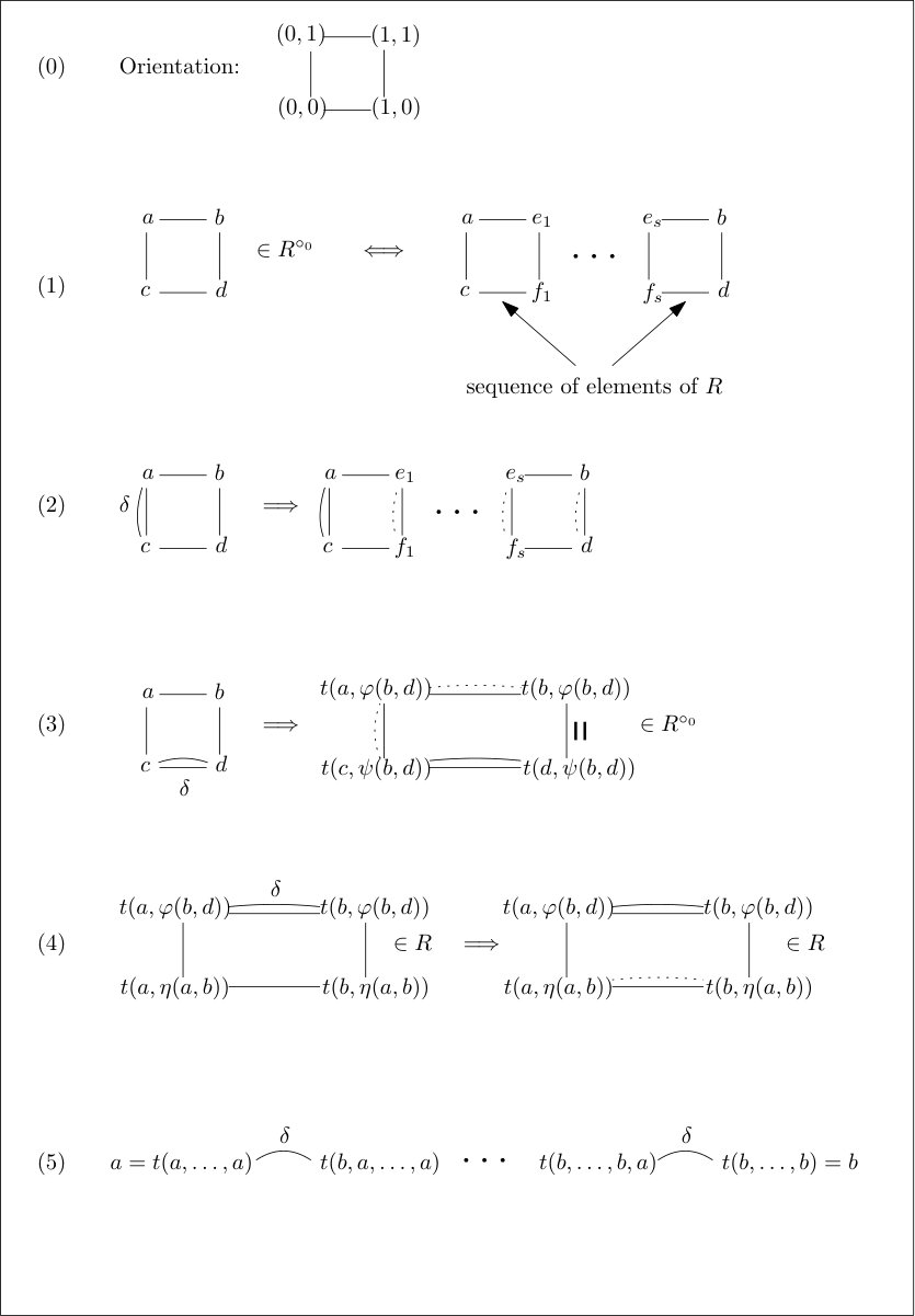 Figure 1
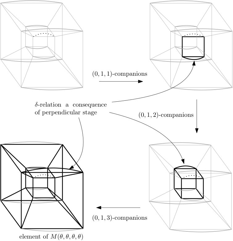 Figure 2
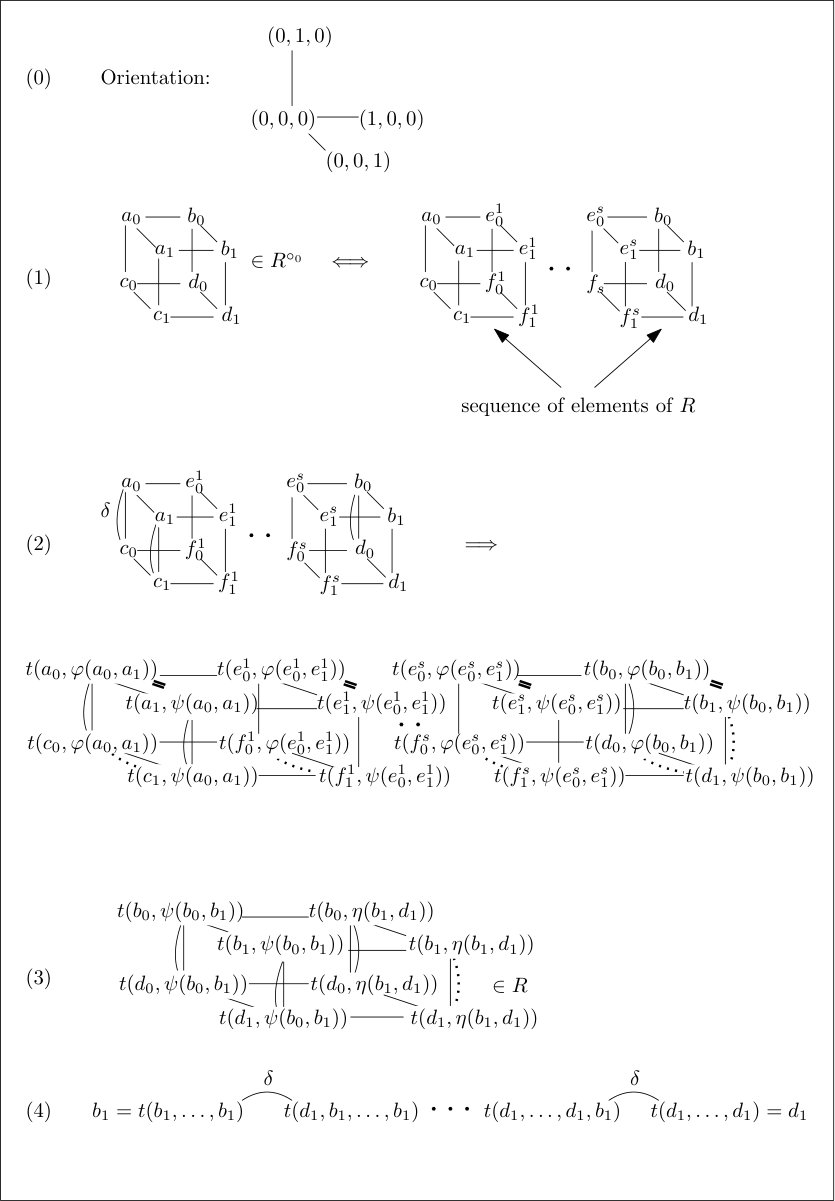 Figure 3
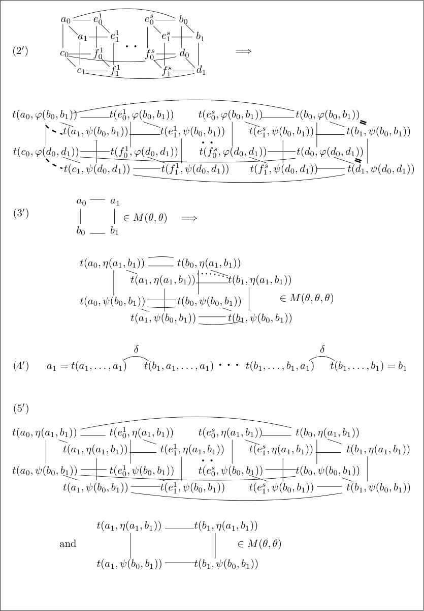 Figure 4
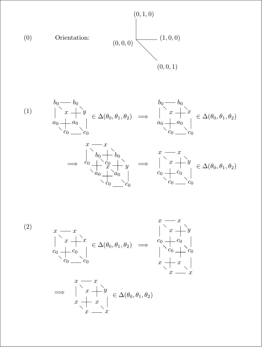 Figure 5
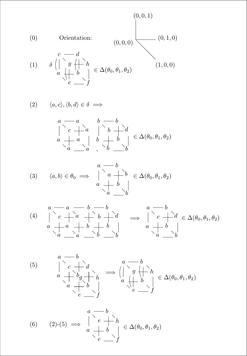 Figure 6
 Figure 7
 Figure 8
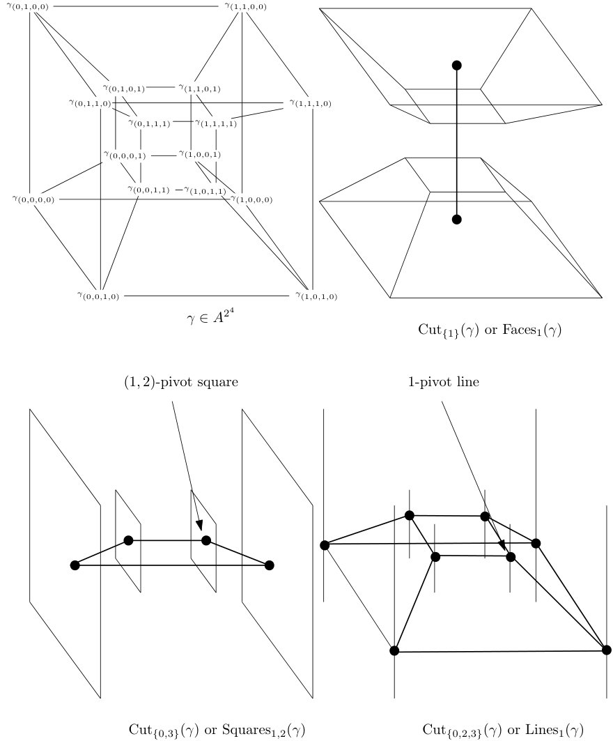 Figure 9
Peer Reviews
No public reviews on file for this paper yet. If you reviewed it on a platform where reviews are public (OpenReview, ICLR, NeurIPS, ICML), you can paste yours below so the community can read it here.
Videos
No videos yet. Explain this paper in a talk, walkthrough, or lecture? Add one.
Supernilpotent Taylor Algebras are Nilpotent
Andrew Moorhead
Department of Mathematics; Vanderbilt University; Nashville, TN; U.S.A.
Abstract.
We develop the theory of the higher commutator for Taylor varieties. A new higher commutator operation called the hypercommutator is defined using a type of invariant relation called a higher dimensional congruence. The hypercommutator is shown to be symmetric and satisfy an inequality relating nested terms. For a Taylor algebra the term condition higher commutator and the hypercommutator are equal when evaluated at a constant tuple, and it follows that every supernilpotent Taylor algebra is nilpotent. We end with a characterization of congruence meet-semidistributive varieties in terms of the neutrality of the higher commutator.
1991 Mathematics Subject Classification:
MSC 08A40 (08A05, 08B05)
This work was supported by the National Science Foundation grant no. DMS 1500254 and the Austrian Science Fund (FWF):P29931
1. Introduction
In this article we study centrality conditions for general algebras. Our goal is to further develop the theory of a congruence lattice operation called the higher commutator, which is a higher arity generalization of the binary commutator. Higher commutator operations are significant because they are used to detect structure that cannot be described with nested binary commutators. An important example is the distinction between nilpotence, which is a condition that is defined using nested binary commutators, and supernilpotence, which is a condition defined using the higher commutator. Until recently, it was not known if supernilpotent algebras are necessarily nilpotent. The answer in general is no [17]. However, we prove here that if a supernilpotent algebra satisfies a nontrivial idempotent equational condition, then the answer is yes. An interesting byproduct of the proof we give is an elementary theory of what we call a higher dimensional congruence.
We begin with a broad outline of the ideas underlying the results of this paper. In 1954 Mal’cev [16] observed that a variety of algebras has permuting congruences exactly when there is a -term satisfying the identities
[TABLE]
A term satisfying these identities is called a Mal’cev operation. His discovery initiated a continuing line of research into the relationship between algebraic structure and equational conditions. Indeed, many important structural features (e.g., congruence modularity, congruence distributivity, etc.) are now known to be enforced by equational laws. The strength of a particular condition may be measured by its position in what is called the lattice of interpretability types of varieties [6]. The collection of all idempotent equational conditions forms a sublattice of the interpretability lattice. Taylor observed [22] that any idempotent variety that does not interpret into the bottom element of this sublattice must have a term satisfying a certain generic package of identities (see the beginning of Section 4). Such a term is called a Taylor term.
Taylor terms have received a lot of attention recently because of their connection to the Constraint Satisfaction Problem. The CSP Dichotomy Conjecture has been independently confirmed by Bulatov [3] and Zhuk [24]. Roughly, each proof demonstrates that if the algebra of operations that preserve a set of finitary relations has a Taylor term, then there is a polynomial time algorithm that decides the CSP for . Using some of algebraic theory that came out of investigating the CSP, Olšák recently proved that any package of Taylor identities force the existence of a particular -ary Taylor term. The results of this article establish that the condition of having a Taylor term has strong consequences for the behavior of higher commutators.
The commutator establishes a useful connection between the possible configurations of an algebra’s invariant relations and its clone of polynomial operations. Smith was the first to articulate such a connection. Using the language of category theory, he developed a signature independent commutator for Mal’cev varieties that interprets as the classical commutator in each of many well known classes, e.g., groups, rings, and Lie algebras [21]. Smith’s idea is a particularly nice example of the kind of insight a study of general algebra provides. The basic operations of an algebra can be thought of as instructions for building structure, and the same structure can be produced in different ways (e.g., a group can be specified in the standard way or as an algebra with a single division operation.) The invariant relations of an algebra are indifferent to the manner in which they are generated, and therefore are the natural place to look for a structural definition of centrality. The language specific definitions of abelianness, solvability, and nilpotence for a particular variety are then consequences of this definition. The success of this viewpoint is demonstrated by Herrmann’s celebrated classification of the abelian algebras belonging to a modular variety as exactly those algebras that are polynomially equivalent to a module [9].
Hagemann and Herrmann were the first to extend Smith’s commutator beyond the domain of Mal’cev varieties. Their development avoided category theory [8] and led to the definition of what is now called the term condition commutator. While the term condition is independent of signature, it is nevertheless a syntactic condition. Freese and McKenzie study commutators for modular varieties in [5]. One of their early conclusions is that all ‘reasonable’ definitions of a commutator for a modular variety are equivalent, and the remainder of the theory developed in the text favors the term condition commutator. A contrasting development of the modular commutator is found in Gumm’s book [7], where the development of the modular commutator is guided by geometrical intuition.
The term condition commutator for a variety that is not modular need not be symmetric, and it follows that two different centrality conditions that are equivalent in the modular case are not equivalent in general. Much is known in spite of this difficulty. In [14], Kearnes and Szendrei prove that the symmetric term condition commutator is equal to the linear commutator for a Taylor variety, and they use this equivalence to prove that any abelian Taylor algebra is polynomially equivalent to a subalgebra of a reduct of a module. We refer the reader to the monograph of Kearnes and Kiss [12] for a thorough treatment of the nonmodular binary commutator.
Bulatov defines a higher arity generalization of the term condition commutator in [4]. While for groups and rings Bulatov’s higher commutator is term definable from the binary commutator, for other Mal’cev algebras it is not (for example, different expansions of a group may share congruences and binary commutators, but have different higher commutator operations). In [2], Aichinger and Mudrinksi develop analogues of those properties shown to be essential for the binary commutator for the higher commutator in a Mal’cev variety. In the same paper the higher commutator is used to define a special subclass of nilpotent Mal’cev algebras, which they call supernilpotent Mal’cev algebras. Using earlier results of Kearnes [11], they go on to show that the finite members of this class are exactly those algebras that are the product of prime power order nilpotent Mal’cev algebras. Supernilpotence has important connections to the free spectrum of an algebra (see for example [1]) and the equation solvability problem (see [10] and[15].) Equation solvability and related problems emphasize the need to understand the differences between nilpotence and supernilpotence.
In [20], Opršal develops properties of the higher commutator in Mal’cev varieties by establishing a connection between the term condition and certain invariant relations. The theory of the higher commutator has been recently extended to varieties that are not Mal’cev. In [18], the author extends most of the theory of the higher commutator to congruence modular varieties. In [19], the author develops a relational description of the modular ternary commutator and uses this to show that -step supernilpotence implies -step nilpotence in a congruence modular variety. In Wires [23], several properties of higher commutators are developed outside of the context of congruence modularity. Implicit in the results of Wires is that supernilpotence implies nilpotence for congruence modular varieties. More recently, Kearnes and Szendrei have announced that any finite supernilpotent algebra is nilpotent, which is to appear in [13].
In the context of current research into the properties of supernilpotent algebras, the main contribution of this article is indicated by its title. However, the machinery that is developed contributes something to the discussion of what a ‘good’ notion of centrality is. In view of the approach to commutator theory taken here, the term condition can be thought of as a local method to check a global condition corresponding to the hypercommutator. This can be compared to the relationship between a tolerance and a congruence. In a Mal’cev variety, these two kinds of relations are the same, but in general one must take the transitive closure of a tolerance to produce a congruence. This is the -dimensional instance of the main idea in this article, which is to extend the notion of transitive closure to a relation that is coordinatized by a hypercube. The success of this local to global principle is determined by the identities in the variety to which it is applied.
The paper is structured as follows. In Section 2 we state some basic definitions and develop enough machinery to define two commutators, which are
- (1)
the term condition commutator, which is written as , and 2. (2)
the * hypercommutator*, which is written as
In Section 4, we prove the two main components of the proof that supernilpotent Taylor algebras are nilpotent. We call these components
- H=TC:
where is a congruence of a Taylor algebra , and 2. HHC8:
for any algebra , , where (cf. HC8 in [2].)
Section 3 is included to illustrate the proof method for few dimensions, and Section 5 examines the behavior of the hypercommutator in a congruence meet-semidistributive variety.
2. Basic Concepts
2.1. Notation
We use the following basic notations. It is convenient for us to always think of the natural numbers as the set of all finite ordinals ordered by set membership. This means we will usually write instead of and instead of . We will usually use the notation to indicate that is a function. We will often (but not always) use subscript notation to indicate images of functions:
[TABLE]
If , then is the notation we use to restrict to . In case the domain of a function is an interval of natural numbers we will also write a function as the tuple .
2.2. Cubes
Let . One of the basic objects we study here are relations of arity . Such relations inherit the structure of an -dimensional cube. This viewpoint allows us to articulate structural properties that would otherwise remain obscure if we considered relations of arity as unstructured tuples.
More generally, let be a finite set of cardinality . An -dimensional cube is the graph with vertices belonging to the set of functions , with two functions connected by an edge when there is exactly one such that . So, a -dimensional cube is a single vertex, a -dimensional cube is two vertices connected by an edge, and so on.
We name some constants of . Denote by i the indicator function that takes value one for and zero elsewhere. Also, denote by 1 the function that takes constant value and 0 the function that takes constant value [math]. It should be clear what the domain is for these constants from the context in which they are used.
Now let be a nonempty set. Formally, every is a collection of pairs and this collection of pairs inherits the structure of a -dimensional cube. That is, let
[TABLE]
be the graph with vertex set , where is connected by an edge to if and only if and are connected in . We will call such a graph a labeled -dimensional cube. The -dimensional cube is a coordinate system for and the value is called the label of the function . We will usually not be so formal and refer to instead of . We denote by -pivot the vertex label . All other vertex labels are called -supporting. Sometimes we call the -supporting vertex label the -antipivot.
By elementary properties of exponents we may decompose any vertex labeled -dimensional cube into a cube of cubes. That is, let and define the map
[TABLE]
So, is a labeled -dimensional cube, where each vertex is labeled by a labeled -dimensional cube which is called a -cut of .
It is easy to see that has an inverse, which is defined as
[TABLE]
Therefore, every labeled -dimensional cube may be represented as a labeled cube of lower dimension, where the vertices of this lower dimensional cube are vertex labeled cubes, and every such cube of cubes may be ‘glued’ back together. It is illustrative to draw pictures of these different representations and we provide some in Figure 1. Note that the labels of some of the vertices are missing to improve readability.
The with such that or are used often enough to merit names:
- (1)
is called , 2. (2)
is called , and 3. (3)
is called .
Now, let be a nonempty set and let . In this situation we say that is a -dimensional relation. The -dimensional cube is a coordinate system for and we think of the elements belonging to as labeled -dimensional cubes. If , we use to denote the set .
To make the notation less cumbersome, we adopt the following convention. If with , then and are isomorphic coordinate systems in the sense any bijection from onto lifts to a graph isomorphism from onto . We will often make use of this fact without mentioning it explicitly.
For example, for let
[TABLE]
be the image of under . Now, and there is an obvious bijection between and . Therefore, we informally treat as a binary relation on the set . In this case we will use a superscript to specify a face, i.e.
[TABLE]
Similarly, let . Because , we informally treat it as a -dimensional cube with vertices labeled by elements of . We will sometimes refer to the vertex labels of as -cross section lines. In this case we call the -pivot line, we call the -antipivot line, and we call any an -supporting line when .
Continuing along these lines, every may be treated as a -dimensional cube with vertices labeled by elements of . We will sometimes refer to the vertex labels of as -cross section squares. We call -pivot the -pivot square of , we call the -antipivot square, and we call an -supporting square when .
Important convention: Whenever we draw a square belonging to , it is always oriented like this picture of \leavevmode\hbox to62.16pt{\vbox to50.99pt{\pgfpicture\makeatletter\hbox{\hskip 12.58333pt\lower-43.98866pt\hbox to0.0pt{\pgfsys@beginscope\pgfsys@invoke{ }\definecolor{pgfstrokecolor}{rgb}{0,0,0}\pgfsys@color@rgb@stroke{0}{0}{0}\pgfsys@invoke{ }\pgfsys@color@rgb@fill{0}{0}{0}\pgfsys@invoke{ }\pgfsys@setlinewidth{0.4pt}\pgfsys@invoke{ }\nullfont\pgfsys@beginscope\pgfsys@invoke{ }\pgfsys@invoke{\lxSVG@closescope }\pgfsys@endscope\hbox to0.0pt{\pgfsys@beginscope\pgfsys@invoke{ }{{}}{{}} {{}}\hbox{\hbox{{\pgfsys@beginscope\pgfsys@invoke{ }{{}{}{{ {}{}}}{ {}{}} {{}{{}}}{{}{}}{}{{}{}} { }{{{{}}\pgfsys@beginscope\pgfsys@invoke{ }\pgfsys@transformcm{1.0}{0.0}{0.0}{1.0}{17.24432pt}{-20.49432pt}\pgfsys@invoke{ }\hbox{{\definecolor{pgfstrokecolor}{rgb}{0,0,0}\pgfsys@color@rgb@stroke{0}{0}{0}\pgfsys@invoke{ }\pgfsys@color@rgb@fill{0}{0}{0}\pgfsys@invoke{ }\hbox{\small{\phantom{\cdot}}} }}\pgfsys@invoke{\lxSVG@closescope }\pgfsys@endscope}}} \pgfsys@invoke{\lxSVG@closescope }\pgfsys@endscope}}} {}{{}}{}{{}}{{}{}}{{}}{}{{}}{{}{}}{{}}{}{{}}{{}{}}{{}}{}{{}}\hbox{\hbox{\hbox{\hbox{\hbox{{\pgfsys@beginscope\pgfsys@invoke{ }{{}{}{{ {}{}}}{ {}{}} {{}{{}}}{{}{}}{}{{}{}} { }{{{{}}\pgfsys@beginscope\pgfsys@invoke{ }\pgfsys@transformcm{1.0}{0.0}{0.0}{1.0}{-10.08333pt}{-2.25pt}\pgfsys@invoke{ }\hbox{{\definecolor{pgfstrokecolor}{rgb}{0,0,0}\pgfsys@color@rgb@stroke{0}{0}{0}\pgfsys@invoke{ }\pgfsys@color@rgb@fill{0}{0}{0}\pgfsys@invoke{ }\hbox{\small{(0,1)}} }}\pgfsys@invoke{\lxSVG@closescope }\pgfsys@endscope}}} \pgfsys@invoke{\lxSVG@closescope }\pgfsys@endscope}}}\hbox{{\pgfsys@beginscope\pgfsys@invoke{ }{{}{}{{ {}{}}}{ {}{}} {{}{{}}}{{}{}}{}{{}{}} { }{{{{}}\pgfsys@beginscope\pgfsys@invoke{ }\pgfsys@transformcm{1.0}{0.0}{0.0}{1.0}{26.90533pt}{-2.25pt}\pgfsys@invoke{ }\hbox{{\definecolor{pgfstrokecolor}{rgb}{0,0,0}\pgfsys@color@rgb@stroke{0}{0}{0}\pgfsys@invoke{ }\pgfsys@color@rgb@fill{0}{0}{0}\pgfsys@invoke{ }\hbox{\small{(1,1)}} }}\pgfsys@invoke{\lxSVG@closescope }\pgfsys@endscope}}} \pgfsys@invoke{\lxSVG@closescope }\pgfsys@endscope}}}\hbox{{\pgfsys@beginscope\pgfsys@invoke{ }{{}{}{{ {}{}}}{ {}{}} {{}{{}}}{{}{}}{}{{}{}} { }{{{{}}\pgfsys@beginscope\pgfsys@invoke{ }\pgfsys@transformcm{1.0}{0.0}{0.0}{1.0}{26.90533pt}{-39.23866pt}\pgfsys@invoke{ }\hbox{{\definecolor{pgfstrokecolor}{rgb}{0,0,0}\pgfsys@color@rgb@stroke{0}{0}{0}\pgfsys@invoke{ }\pgfsys@color@rgb@fill{0}{0}{0}\pgfsys@invoke{ }\hbox{\small{(1,0)}} }}\pgfsys@invoke{\lxSVG@closescope }\pgfsys@endscope}}} \pgfsys@invoke{\lxSVG@closescope }\pgfsys@endscope}}}\hbox{{\pgfsys@beginscope\pgfsys@invoke{ }{{}{}{{ {}{}}}{ {}{}} {{}{{}}}{{}{}}{}{{}{}} { }{{{{}}\pgfsys@beginscope\pgfsys@invoke{ }\pgfsys@transformcm{1.0}{0.0}{0.0}{1.0}{-10.08333pt}{-39.23866pt}\pgfsys@invoke{ }\hbox{{\definecolor{pgfstrokecolor}{rgb}{0,0,0}\pgfsys@color@rgb@stroke{0}{0}{0}\pgfsys@invoke{ }\pgfsys@color@rgb@fill{0}{0}{0}\pgfsys@invoke{ }\hbox{\small{(0,0)}} }}\pgfsys@invoke{\lxSVG@closescope }\pgfsys@endscope}}} \pgfsys@invoke{\lxSVG@closescope }\pgfsys@endscope}}} { {}{}{}}{}{ {}{}{}} {{{{{}}{ {}{}}{}{}{{}{}}}}}{}{{{{{}}{ {}{}}{}{}{{}{}}}}}{{}}{}{}{}{ {}{}{}} {{{{{}}{ {}{}}{}{}{{}{}}}}}{}{{{{{}}{ {}{}}{}{}{{}{}}}}}{{}}{}{}{}{ {}{}{}} {{{{{}}{ {}{}}{}{}{{}{}}}}}{}{{{{{}}{ {}{}}{}{}{{}{}}}}}{{}}{}{}{}{ {}{}{}} {{{{{}}{ {}{}}{}{}{{}{}}}}}{}{{{{{}}{ {}{}}{}{}{{}{}}}}}{{}}{}{}{}{}\pgfsys@moveto{12.78325pt}{0.0pt}\pgfsys@lineto{24.20523pt}{0.0pt}\pgfsys@moveto{36.98851pt}{-7.19995pt}\pgfsys@lineto{36.98851pt}{-29.78854pt}\pgfsys@moveto{24.20523pt}{-36.98851pt}\pgfsys@lineto{12.78325pt}{-36.98851pt}\pgfsys@moveto{0.0pt}{-29.78854pt}\pgfsys@lineto{0.0pt}{-7.19995pt}\pgfsys@stroke\pgfsys@invoke{ } \pgfsys@invoke{\lxSVG@closescope }\pgfsys@endscope{{ {}{}{}}}{}{}\hss}\pgfsys@discardpath\pgfsys@invoke{\lxSVG@closescope }\pgfsys@endscope\hss}}\lxSVG@closescope\endpgfpicture}}, along with the convention that corresponds to and corresponds to . According to this scheme, a picture of an element in is the transpose of a picture of an element in .
2.3. Higher Dimensional Congruence Relations
Definition 2.1**.**
Let be a nonempty set and let be a binary relation on . We say that is a quasiequivalence relation on provided that each of the following conditions hold:
- (1)
implies (quasireflexivity), 2. (2)
if and only if . (symmetry), and 3. (3)
imply that (transitivity).
Definition 2.2**.**
Let be an algebra with underlying set and let be a -dimensional relation for some .
- (1)
is said to be -reflexive, -symmetric, or -transitive if
is respectively quasireflexive, symmetric, or transitive on for each . 2. (2)
is said to be a -dimensional equivalence relation provided
is a quasiequivalence relation on for each . 3. (3)
is said to be a -dimensional congruence of if it is a -dimensional equivalence that is also compatible with the basic operation of . 4. (4)
is said to be a -dimensional tolerance of if it is -reflexive, -symmetric, and compatible with the basic operations of .
The higher dimensional versions of reflexivity and symmetry can be described in terms of certain unary operations. Let be a nonempty set, , and . For each , we define the maps and by
[TABLE]
The following lemma is an easy consequence of the definitions.
Lemma 2.3**.**
Let be a nonempty set and . Let be a -dimensional relation. The following hold:
- (1)
* is -reflexive if and only if is closed under for all , and* 2. (2)
* is -symmetric if and only if is closed under for every .*
We observed earlier that any vertex labeled -dimensional cube can be interpreted as a cube of cubes. Such an interpretation may be used to formulate weaker versions of higher dimensional symmetry, reflexivity and transitivity. The following lemma makes this precise. The proof, which involves a direct application of the definitions, is left to the reader.
Lemma 2.4**.**
Let be a nonempty set and . Let and suppose . Each of the following implications holds.
- (1)
If is -symmetric, then is -symmetric. 2. (2)
If is -reflexive, then is -reflexive. 3. (3)
If is -transitive, then is -transitive.
Corollary 2.5**.**
Let be a nonempty set, , and be a -dimensional relation. Let , and . Let be defined by for every . If is -reflexive, then .
Proof.
Suppose for . We first prove the lemma in the special case when . In this case . Let . The lemma is asserting that , where is defined by for all . Indeed, it is clear that
[TABLE]
Because is assumed to be -reflexive, it follows from Lemma 2.3 that .
For the general case we apply the special case we just handled to the situation where , , , and . Now let be defined by . We suppose that is -reflexive, so Lemma 2.4 shows that is -reflexive. All of the assumptions we made in the special case are satisfied, so we conclude that . Because , we have shown that , or equivalently, that .
∎
The properties of -symmetry, reflexivity, and transitivity are each preserved by projecting onto a set of coordinates that determines a lower dimensional cube. This feature, which is made precise in the next lemma, is in a sense dual to the situation described in Lemma 2.4.
Lemma 2.6**.**
Let be a nonempty set and . Let and suppose . Take . Each of the following implications holds.
- (1)
If is -symmetric, then is -symmetric. 2. (2)
If is -reflexive, then is -reflexive. 3. (3)
If is -transitive and -reflexive, then is -transitive.
Proof.
The proof of (1) and (2) is left to the reader. We prove (3). Suppose the conditions of the lemma and (3) hold and let be such that for some . We show that . Let be defined by and , for all . Applying Corollary 2.5 to this situation shows that .
We claim that . Indeed, let . We can decompose as the union of two partial functions and . The computation
[TABLE]
establishes our claim. Therefore, and so . A computation similar to the one above shows that , as desired.
∎
Corollary 2.7**.**
Let be an algebra and . Let be a -dimensional tolerance of . For every ,
- (1)
* is a -dimensional tolerance of , and* 2. (2)
* for all .*
Additionally, the same statement holds if the word ‘tolerance’ is replaced by ‘congruence’.
Proof.
The first item (1) of the lemma follows from (1) and (2) of Lemma 2.6. To show (2), suppose and take . By Corollary 2.5, there exists so that . Therefore, . The same argument shows that .
If is assumed to be a -dimensional congruence, then (3) of Lemma 2.6 indicates that is also -transitive for every . This establishes the final statement of the lemma. ∎
Definition 2.8**.**
Let be an algebra. For each , set
[TABLE]
- (1)
2. (2)
.
It is an easy exercise to show that each of these lattices is algebraic. The definition we give contains many redundancies, because and encode exactly the same information whenever . The reader may wonder why we do not instead use the canonical choice of coordinates which produces the following sequence of lattices:
[TABLE]
Our choice is motivated by a wish to avoid changing coordinate systems when we consider nested commutator expressions.
We remark that is different from , because we require only quasireflexivity of our relations. This relaxation of reflexivity has the consequence that contains all congruences of subalgebras of . The ordinary congruence lattice of is isomorphic to the interval above the full diagonal relation in . We also remark that is the lattice of subuniverses of and that all of these lattices may have the empty relation as the least element in the event that has no smallest subalgebra. There are some appealing extensions of classical results pertaining to congruences to higher dimensional congruences. Most notably, an -dimensional equivalence relation of an algebra is a compatible relation if and only if it is compatible with those -ary polynomials of the subalgebra determined by its intersection with the diagonal of in . These ideas will be presented in a companion article.
We now describe the generation of higher dimensional congruences. Take (the case is generation of a subalgebra), and let . We respectively define the -dimensional congruence and -dimensional tolerance of generated by as
[TABLE]
The notion of a transitive closure of a binary relation generalizes to higher dimensions in the obvious way. Suppose for some . Let be a -dimensional relation. For set
[TABLE]
where is the transitive closure of when interpreted as a binary relation. We recursively define
- (1)
, and 2. (2)
, for .
Finally, set . The proof of the following proposition is left to the reader.
Lemma 2.9**.**
Let be an algebra and . The following hold.
- (1)
If is a -dimensional tolerance of , then is a -dimensional tolerance of and . 2. (2)
, for all . 3. (3)
, for all , , and .
2.4. Centrality Conditions
We now use this machinery to develop the commutator theory for the congruences of an algebra. It is interesting to note that the scope of this theory could be enlarged to include all higher dimensional congruences. It is unclear if such a broad generalization of commutator theory has any practical application, so we limit our development to congruences.
In this section we define two centralizer conditions that are used to define two distinct higher arity commutators. The first is due to Bulatov and is a natural extension of the so-called term condition. The second is a new condition and is used to define what we call the hypercommutator.
The definition of the -ary commutator as formulated by Bulatov in [4] can be restated as a condition on a certain -dimensional invariant relation, elements of which are often referred to as matrices. We do not state the original definition here, but refer the reader to [18] for details on the equivalence between our definition of the term condition higher commutator and that given by Bulatov.
Let be an algebra, , and . Corollary 2.7 associates to any -dimensional congruence a collection of -dimensional congruences indexed by the subsets of of cardinality , i.e. the set
[TABLE]
For any such indexed set of higher dimensional congruences, i.e.
[TABLE]
there exists (as can be easily verified) a maximal -dimensional congruence
[TABLE]
that satisfies
[TABLE]
We call this maximal relation the -rectangles. In the special case that , we have that is an -indexed family of -dimensional congruences, and is the -dimensional congruence consisting of all those satisfying , for all and . If it is also the case that , we use the notation
[TABLE]
We are still in the situation where is an algebra and . Assume also that . For each define by
[TABLE]
From the context it should be clear what the dimension of is.
Definition 2.10**.**
Let be an algebra and with . Let be an -indexed set of congruences. Set
[TABLE]
Notice that if , then and this relation is equal to (up to a trivial change of coordinates). In case , we will use the notation , , and for , , and , respectively.
Remark*.*
Let . For each , the map
[TABLE]
when restricted to is a lattice embedding into . Denote the least congruence of by [math]. Any two distinct such embeddings intersect only at their shared bottom element, which is . See Figure 2 for a picture that shows the relationship between these embeddings and Definition 2.10.
For historical reasons, we call the algebra of matrices. The following lemmas establish some basic properties of these two relations. Each statement is referring to the situation established in Definition 2.10.
Lemma 2.11**.**
**
Proof.
The first containment follows from the fact that any -dimensional congruence is also a -dimensional tolerance. The second containment follows from the observation that and that . ∎
Lemma 2.12**.**
M(\{\theta_{i}\}_{i\in S})=\operatorname{Sg}_{A^{2^{S}}}\bigg{(}\bigcup_{i\in S}\operatorname{cube}_{i}(\theta_{i})\bigg{)}.**
Proof.
Because is a congruence for each , the relation is both -symmetric and -reflexive. It follows that
[TABLE]
is already an -dimensional tolerance, and is therefore equal to . ∎
Lemma 2.13**.**
.
Proof.
This is an immediate consequence of Lemma 2.9. ∎
Lemma 2.14**.**
For every and ,
- (1)
, and 2. (2)
.
Proof.
We first notice that commutes with the term operations of . That is, for every term and . Furthermore, we compute
[TABLE]
To establish (1), we apply Lemma 2.12 and conclude that
[TABLE]
To establish (2), we show that each of the two relations contains the other. Suppose that . It follows from Lemma 2.13 that . We now apply (3) of Lemma 2.9 and conclude that
[TABLE]
Therefore, . For the other containment, we first note that , so
[TABLE]
Corollary 2.7 indicates that is a -dimensional congruence of . Therefore,
∎
Definition 2.15**.**
Let be an algebra, , with , and . We say that a -dimensional relation on has -centrality if there is no such that exactly many vertices of are labeled by -pairs.
The relations that we consider here are usually -symmetric. In this situation, the following lemma provides a useful method to check centrality. The proof is left to the reader.
Lemma 2.16**.**
Let be an algebra, , with , and . Suppose that a -dimensional relation is -symmetric. Then has -centrality if and only if the following condition holds:
If is such that every -supporting line of is a -pair, then the -pivot line of is also a -pair.
We now define two commutators. They share one essential feature: both are defined with respect to a centrality condition that is quantified over an -dimensional relation for some .
Definition 2.17**.**
Let be an algebra and with . Let be an -indexed set of congruences. Let be the greatest element of . We define
[TABLE]
We call these operations the -ary term condition commutator and hypercommutator, respectively. In case , we use the notation and for these operations.
Theorem 2.18**.**
Let be an algebra, , and with . The following hold for both the term condition commutator and the hypercommutator:
- (1)
, 2. (2)
, and 3. (3)
**
The following also holds:
- (4)
**
Proof.
Properties (1)-(3) are already known to hold for the term condition commutator, see [2]. Let us establish that they hold for the hypercommutator.
To show (1), set . We must verify that has -centrality, and will apply the criterion established by Lemma 2.16 to do so. Take
with the property that every -supporting line is a -pair. We want to show that the -pivot line of is a -pair, for every . This holds for , because Lemma 2.11 indicates that . For , consider the -pivot square
[TABLE]
The pair is an -supporting line of and is therefore a -pair. We have indicated this with a curved line. The -pivot line of is the pair . Because , it follows that . Therefore, .
To show (2) and (4), it is enough to note that
[TABLE]
and that the set \{R\subseteq A^{2^{n}}:\text{R(\delta,n-1)-centrality}\} is downward closed, for every .
To see that (3) holds, suppose that is such that has -centrality. Take such that every -supporting line of is a -pair. It follows that every -supporting line of is a -pair. Lemma 2.14 indicates that . We apply the assumption that has -centrality and conclude that is a -pair. We have shown that also has -centrality, so the proof is finished. ∎
2.5. Nilpotence and Supernilpotence
Let be an algebra and let . Recursively define over the congruences , and
[TABLE]
to produce a descending chain called the lower central series of :
[TABLE]
If , then is said to be -step left nilpotent. A congruence of is said to be -step supernilpotent if it satisfies
[TABLE]
3. The binary and ternary cases
3.1. Proof of H=TC for the binary and ternary cases
Theorem 2.18 indicates that the hypercommutator is always an upper bound for the term condition commutator of the same arity. In this section we will show that
[TABLE]
if is a congruence of a Taylor algebra (see the beginning of Section 4.) Indeed, we will demonstrate that has -centrality for each whenever has -centrality for each . The idea for the proof will generalize to any dimension. We want to point out that the key to the argument is inspired by Lemma 4.4 in [14].
Lemma 3.1**.**
Let be a variety with Taylor term . Let , , and . Suppose is a -dimensional tolerance of such that and has -centrality for each . Then, has -centrality for each .
Proof.
We assume without loss assume that . The proof will refer to the items listed in Figure 3. Before we begin, we remark that item shows the orientation of coordinates, and that any pair of elements that belongs to is connected with a curved line. A typical element of is shown in item . Now assume that , as shown in item . An induction using that has -centrality is illustrated with dotted curved lines, and it follows that . Therefore, has -centrality.
Next we show that has -centrality. Assume that , as depicted on the left-hand side of the implication depicted in item . Suppose that the Taylor identity that satisfies in its first coordinate is given by
[TABLE]
where and denote tuples in the variables . It follows from the compatibility, -reflexivity, and -symmetry of that the right-hand side of the implication depicted in item belongs to . We observed earlier that has -centrality, and this along with the equality implies that . Therefore, all of the labels of this square belong to the same -class. In particular, we conclude that is a -pair.
Now, let . Because , we know that all belong to the same -class. We assume also that , hence the square shown in item (4) belongs to . Because is assumed to have -centrality, we conclude that is a -pair.
This line of reasoning can be duplicated for each coordinate of the Taylor term . Therefore, we construct a -chain that connects to , see item . This demonstrates that has -centrality.
∎
Theorem 3.2**.**
For be a Taylor variety, , and ,
[TABLE]
Proof.
By Theorem 2.18, the binary hypercommutator always lies above the binary term condition commutator. We show that . Set . It suffices to check that has -centrality, for each .
We proceed by induction. For each set . It follows inductively from (1) of Lemma 2.9 that each is a -dimensional tolerance such that . Using this, it follows inductively from Lemma 3.1 that each has -centrality for all . Because the proof is finished. ∎
The proof of Theorem 3.2 has a structure which provides a template for the higher arity cases. The following is a list of the essential steps and their names.
- (1)
Inductive Assumption: Assume that is an -dimensional tolerance such that and has -centrality for all . 2. (2)
Perpendicular Stage: Establish that has -centrality for . 3. (3)
Parallel Stage: Establish that has -centrality.
Next, we illustrate this proof template in the -dimensional case.
Lemma 3.3**.**
Let be a variety with Taylor term and let . Let and . Let be a -dimensional relation such that and has -centrality for each . Then, the relation has -centrality for each .
Proof.
The main steps of the proof are illustrated in Figures 4 and 5. Without loss, we assume that . We begin with the perpendicular stage and refer to Figure 4. Item illustrates the orientation of coordinates. We want to show that has -centrality for each . Without loss, take . A typical element of is depicted in item . The left hand side of the implication in item illustrates the assumption that
[TABLE]
We want to show that . Suppose that the identity that satisfies in the first coordinate is given by
[TABLE]
where and denote tuples in the variables . The right hand side of the implication in item depicts a sequence of elements of , the corners of which determine a cube that belongs to . Each solid curved line indicates that the corresponding vertex labels determine a -pair, while the symbol along each top row indicates an equality that results from an application of the Taylor identity. The curved dotted lines also indicate -pairs. Their existence is deduced left-to-right, first by the transitivity of , then by an application of the -centrality of , and last by an application of the transitivity of . We conclude that
[TABLE]
Let . The labeled cube depicted in item is an element of . This follows because the labeled cube determined by the first argument of belongs to (because is -symmetric), as do the labeled cubes determined by each of the remaining arguments of (because .) The two columns belonging to the back face determine -pairs because , and it has been shown that the left column of the front face also determines a -pair. Because has -centrality, we conclude that
[TABLE]
Item (4) finishes the argument in a manner identical to the end of the proof of Lemma 3.1. This finishes the perpendicular stage of the argument.
We proceed to the parallel stage and refer to Figure 5. The left hand side of the implication in item illustrates the assumption that
[TABLE]
We want to show that . As before, we present an argument involving the first argument of the Taylor term. The right hand side of the implication in item depicts a sequence of elements of , the corners of which determine a cube that belongs to . A solid curved line indicates a -pair whose existence follows from the initial assumptions. The dotted curved lines also indicate -pairs. The existence of the bottom dotted curved line follows from the transitivity of , while the existence of the top dotted curved line follows from our earlier completion of the perpendicular stage. We conclude that
[TABLE]
Now, let . As before, our goal is to show that
[TABLE]
We need to produce an element of to which we may apply the assumption that has -centrality for each . This is possible provided we assume that
[TABLE]
as illustrated in item . The remainder of the argument in this case is similar to the perpendicular stage.
In general, we may only produce the sequence of elements of shown in item . Because this is another instance of the parallel stage, it appears as though no progress has been made. However, note that there is a symmetric version of in which we assume that
[TABLE]
This new instance satisfies assumptions of this symmetric version of , so we conclude that
[TABLE]
This finishes the proof of the parallel stage. ∎
The analogue of Theorem 3.2 immediately follows. Because it is a special case of Theorem 4.9, we omit the proof.
Theorem 3.4**.**
Let be a Taylor variety, , and . In this situation,
[TABLE]
3.2. Proof of HHC8 for the binary and ternary case
Let be any algebra and take . We will show that
[TABLE]
We begin by developing a relational characterization of both the binary and ternary hypercommutators. Both Propositions 3.5 and 3.6 are special cases of Theorem 4.10.
Proposition 3.5**.**
Let be an algebra and take . The following are equivalent.
- (1)
. 2. (2)
\leavevmode\hbox to38.6pt{\vbox to38.2pt{\pgfpicture\makeatletter\hbox{\hskip 5.07187pt\lower-32.89024pt\hbox to0.0pt{\pgfsys@beginscope\pgfsys@invoke{ }\definecolor{pgfstrokecolor}{rgb}{0,0,0}\pgfsys@color@rgb@stroke{0}{0}{0}\pgfsys@invoke{ }\pgfsys@color@rgb@fill{0}{0}{0}\pgfsys@invoke{ }\pgfsys@setlinewidth{0.4pt}\pgfsys@invoke{ }\nullfont\pgfsys@beginscope\pgfsys@invoke{ }\pgfsys@invoke{\lxSVG@closescope }\pgfsys@endscope\hbox to0.0pt{\pgfsys@beginscope\pgfsys@invoke{ }{{}}{{}} {{}}\hbox{\hbox{{\pgfsys@beginscope\pgfsys@invoke{ }{{}{}{{ {}{}}}{ {}{}} {{}{{}}}{{}{}}{}{{}{}} { }{{{{}}\pgfsys@beginscope\pgfsys@invoke{ }\pgfsys@transformcm{1.0}{0.0}{0.0}{1.0}{12.97638pt}{-16.22638pt}\pgfsys@invoke{ }\hbox{{\definecolor{pgfstrokecolor}{rgb}{0,0,0}\pgfsys@color@rgb@stroke{0}{0}{0}\pgfsys@invoke{ }\pgfsys@color@rgb@fill{0}{0}{0}\pgfsys@invoke{ }\hbox{\small{\phantom{\cdot}}} }}\pgfsys@invoke{\lxSVG@closescope }\pgfsys@endscope}}} \pgfsys@invoke{\lxSVG@closescope }\pgfsys@endscope}}} {}{{}}{}{{}}{{}{}}{{}}{}{{}}{{}{}}{{}}{}{{}}{{}{}}{{}}{}{{}}\hbox{\hbox{\hbox{\hbox{\hbox{{\pgfsys@beginscope\pgfsys@invoke{ }{{}{}{{ {}{}}}{ {}{}} {{}{{}}}{{}{}}{}{{}{}} { }{{{{}}\pgfsys@beginscope\pgfsys@invoke{ }\pgfsys@transformcm{1.0}{0.0}{0.0}{1.0}{-2.57187pt}{-1.93748pt}\pgfsys@invoke{ }\hbox{{\definecolor{pgfstrokecolor}{rgb}{0,0,0}\pgfsys@color@rgb@stroke{0}{0}{0}\pgfsys@invoke{ }\pgfsys@color@rgb@fill{0}{0}{0}\pgfsys@invoke{ }\hbox{\small{x}} }}\pgfsys@invoke{\lxSVG@closescope }\pgfsys@endscope}}} \pgfsys@invoke{\lxSVG@closescope }\pgfsys@endscope}}}\hbox{{\pgfsys@beginscope\pgfsys@invoke{ }{{}{}{{ {}{}}}{ {}{}} {{}{{}}}{{}{}}{}{{}{}} { }{{{{}}\pgfsys@beginscope\pgfsys@invoke{ }\pgfsys@transformcm{1.0}{0.0}{0.0}{1.0}{26.08504pt}{-1.06248pt}\pgfsys@invoke{ }\hbox{{\definecolor{pgfstrokecolor}{rgb}{0,0,0}\pgfsys@color@rgb@stroke{0}{0}{0}\pgfsys@invoke{ }\pgfsys@color@rgb@fill{0}{0}{0}\pgfsys@invoke{ }\hbox{\small{y}} }}\pgfsys@invoke{\lxSVG@closescope }\pgfsys@endscope}}} \pgfsys@invoke{\lxSVG@closescope }\pgfsys@endscope}}}\hbox{{\pgfsys@beginscope\pgfsys@invoke{ }{{}{}{{ {}{}}}{ {}{}} {{}{{}}}{{}{}}{}{{}{}} { }{{{{}}\pgfsys@beginscope\pgfsys@invoke{ }\pgfsys@transformcm{1.0}{0.0}{0.0}{1.0}{25.88089pt}{-30.39024pt}\pgfsys@invoke{ }\hbox{{\definecolor{pgfstrokecolor}{rgb}{0,0,0}\pgfsys@color@rgb@stroke{0}{0}{0}\pgfsys@invoke{ }\pgfsys@color@rgb@fill{0}{0}{0}\pgfsys@invoke{ }\hbox{\small{x}} }}\pgfsys@invoke{\lxSVG@closescope }\pgfsys@endscope}}} \pgfsys@invoke{\lxSVG@closescope }\pgfsys@endscope}}}\hbox{{\pgfsys@beginscope\pgfsys@invoke{ }{{}{}{{ {}{}}}{ {}{}} {{}{{}}}{{}{}}{}{{}{}} { }{{{{}}\pgfsys@beginscope\pgfsys@invoke{ }\pgfsys@transformcm{1.0}{0.0}{0.0}{1.0}{-2.57187pt}{-30.39024pt}\pgfsys@invoke{ }\hbox{{\definecolor{pgfstrokecolor}{rgb}{0,0,0}\pgfsys@color@rgb@stroke{0}{0}{0}\pgfsys@invoke{ }\pgfsys@color@rgb@fill{0}{0}{0}\pgfsys@invoke{ }\hbox{\small{x}} }}\pgfsys@invoke{\lxSVG@closescope }\pgfsys@endscope}}} \pgfsys@invoke{\lxSVG@closescope }\pgfsys@endscope}}} { {}{}{}}{}{ {}{}{}} {{{{{}}{ {}{}}{}{}{{}{}}}}}{}{{{{{}}{ {}{}}{}{}{{}{}}}}}{{}}{}{}{}{ {}{}{}} {{{{{}}{ {}{}}{}{}{{}{}}}}}{}{{{{{}}{ {}{}}{}{}{{}{}}}}}{{}}{}{}{}{ {}{}{}} {{{{{}}{ {}{}}{}{}{{}{}}}}}{}{{{{{}}{ {}{}}{}{}{{}{}}}}}{{}}{}{}{}{ {}{}{}} {{{{{}}{ {}{}}{}{}{{}{}}}}}{}{{{{{}}{ {}{}}{}{}{{}{}}}}}{{}}{}{}{}{}\pgfsys@moveto{5.27187pt}{0.0pt}\pgfsys@lineto{23.38504pt}{0.0pt}\pgfsys@moveto{28.45276pt}{-5.51248pt}\pgfsys@lineto{28.45276pt}{-23.81528pt}\pgfsys@moveto{23.1809pt}{-28.45276pt}\pgfsys@lineto{5.27187pt}{-28.45276pt}\pgfsys@moveto{0.0pt}{-23.81528pt}\pgfsys@lineto{0.0pt}{-4.63748pt}\pgfsys@stroke\pgfsys@invoke{ } \pgfsys@invoke{\lxSVG@closescope }\pgfsys@endscope{{ {}{}{}}}{}{}\hss}\pgfsys@discardpath\pgfsys@invoke{\lxSVG@closescope }\pgfsys@endscope\hss}}\lxSVG@closescope\endpgfpicture}}\in\Delta(\theta_{0},\theta_{1}). 3. (3)
\leavevmode\hbox to38.4pt{\vbox to38.2pt{\pgfpicture\makeatletter\hbox{\hskip 4.87865pt\lower-32.89024pt\hbox to0.0pt{\pgfsys@beginscope\pgfsys@invoke{ }\definecolor{pgfstrokecolor}{rgb}{0,0,0}\pgfsys@color@rgb@stroke{0}{0}{0}\pgfsys@invoke{ }\pgfsys@color@rgb@fill{0}{0}{0}\pgfsys@invoke{ }\pgfsys@setlinewidth{0.4pt}\pgfsys@invoke{ }\nullfont\pgfsys@beginscope\pgfsys@invoke{ }\pgfsys@invoke{\lxSVG@closescope }\pgfsys@endscope\hbox to0.0pt{\pgfsys@beginscope\pgfsys@invoke{ }{{}}{{}} {{}}\hbox{\hbox{{\pgfsys@beginscope\pgfsys@invoke{ }{{}{}{{ {}{}}}{ {}{}} {{}{{}}}{{}{}}{}{{}{}} { }{{{{}}\pgfsys@beginscope\pgfsys@invoke{ }\pgfsys@transformcm{1.0}{0.0}{0.0}{1.0}{12.97638pt}{-16.22638pt}\pgfsys@invoke{ }\hbox{{\definecolor{pgfstrokecolor}{rgb}{0,0,0}\pgfsys@color@rgb@stroke{0}{0}{0}\pgfsys@invoke{ }\pgfsys@color@rgb@fill{0}{0}{0}\pgfsys@invoke{ }\hbox{\small{\phantom{\cdot}}} }}\pgfsys@invoke{\lxSVG@closescope }\pgfsys@endscope}}} \pgfsys@invoke{\lxSVG@closescope }\pgfsys@endscope}}} {}{{}}{}{{}}{{}{}}{{}}{}{{}}{{}{}}{{}}{}{{}}{{}{}}{{}}{}{{}}\hbox{\hbox{\hbox{\hbox{\hbox{{\pgfsys@beginscope\pgfsys@invoke{ }{{}{}{{ {}{}}}{ {}{}} {{}{{}}}{{}{}}{}{{}{}} { }{{{{}}\pgfsys@beginscope\pgfsys@invoke{ }\pgfsys@transformcm{1.0}{0.0}{0.0}{1.0}{-2.37865pt}{-1.93748pt}\pgfsys@invoke{ }\hbox{{\definecolor{pgfstrokecolor}{rgb}{0,0,0}\pgfsys@color@rgb@stroke{0}{0}{0}\pgfsys@invoke{ }\pgfsys@color@rgb@fill{0}{0}{0}\pgfsys@invoke{ }\hbox{\small{a}} }}\pgfsys@invoke{\lxSVG@closescope }\pgfsys@endscope}}} \pgfsys@invoke{\lxSVG@closescope }\pgfsys@endscope}}}\hbox{{\pgfsys@beginscope\pgfsys@invoke{ }{{}{}{{ {}{}}}{ {}{}} {{}{{}}}{{}{}}{}{{}{}} { }{{{{}}\pgfsys@beginscope\pgfsys@invoke{ }\pgfsys@transformcm{1.0}{0.0}{0.0}{1.0}{26.08504pt}{-1.06248pt}\pgfsys@invoke{ }\hbox{{\definecolor{pgfstrokecolor}{rgb}{0,0,0}\pgfsys@color@rgb@stroke{0}{0}{0}\pgfsys@invoke{ }\pgfsys@color@rgb@fill{0}{0}{0}\pgfsys@invoke{ }\hbox{\small{y}} }}\pgfsys@invoke{\lxSVG@closescope }\pgfsys@endscope}}} \pgfsys@invoke{\lxSVG@closescope }\pgfsys@endscope}}}\hbox{{\pgfsys@beginscope\pgfsys@invoke{ }{{}{}{{ {}{}}}{ {}{}} {{}{{}}}{{}{}}{}{{}{}} { }{{{{}}\pgfsys@beginscope\pgfsys@invoke{ }\pgfsys@transformcm{1.0}{0.0}{0.0}{1.0}{25.88089pt}{-30.39024pt}\pgfsys@invoke{ }\hbox{{\definecolor{pgfstrokecolor}{rgb}{0,0,0}\pgfsys@color@rgb@stroke{0}{0}{0}\pgfsys@invoke{ }\pgfsys@color@rgb@fill{0}{0}{0}\pgfsys@invoke{ }\hbox{\small{x}} }}\pgfsys@invoke{\lxSVG@closescope }\pgfsys@endscope}}} \pgfsys@invoke{\lxSVG@closescope }\pgfsys@endscope}}}\hbox{{\pgfsys@beginscope\pgfsys@invoke{ }{{}{}{{ {}{}}}{ {}{}} {{}{{}}}{{}{}}{}{{}{}} { }{{{{}}\pgfsys@beginscope\pgfsys@invoke{ }\pgfsys@transformcm{1.0}{0.0}{0.0}{1.0}{-2.37865pt}{-30.39024pt}\pgfsys@invoke{ }\hbox{{\definecolor{pgfstrokecolor}{rgb}{0,0,0}\pgfsys@color@rgb@stroke{0}{0}{0}\pgfsys@invoke{ }\pgfsys@color@rgb@fill{0}{0}{0}\pgfsys@invoke{ }\hbox{\small{a}} }}\pgfsys@invoke{\lxSVG@closescope }\pgfsys@endscope}}} \pgfsys@invoke{\lxSVG@closescope }\pgfsys@endscope}}} { {}{}{}}{}{ {}{}{}} {{{{{}}{ {}{}}{}{}{{}{}}}}}{}{{{{{}}{ {}{}}{}{}{{}{}}}}}{{}}{}{}{}{ {}{}{}} {{{{{}}{ {}{}}{}{}{{}{}}}}}{}{{{{{}}{ {}{}}{}{}{{}{}}}}}{{}}{}{}{}{ {}{}{}} {{{{{}}{ {}{}}{}{}{{}{}}}}}{}{{{{{}}{ {}{}}{}{}{{}{}}}}}{{}}{}{}{}{ {}{}{}} {{{{{}}{ {}{}}{}{}{{}{}}}}}{}{{{{{}}{ {}{}}{}{}{{}{}}}}}{{}}{}{}{}{}\pgfsys@moveto{5.07864pt}{0.0pt}\pgfsys@lineto{23.38504pt}{0.0pt}\pgfsys@moveto{28.45276pt}{-5.51248pt}\pgfsys@lineto{28.45276pt}{-23.81528pt}\pgfsys@moveto{23.1809pt}{-28.45276pt}\pgfsys@lineto{5.07864pt}{-28.45276pt}\pgfsys@moveto{0.0pt}{-23.81528pt}\pgfsys@lineto{0.0pt}{-4.63748pt}\pgfsys@stroke\pgfsys@invoke{ } \pgfsys@invoke{\lxSVG@closescope }\pgfsys@endscope{{ {}{}{}}}{}{}\hss}\pgfsys@discardpath\pgfsys@invoke{\lxSVG@closescope }\pgfsys@endscope\hss}}\lxSVG@closescope\endpgfpicture}}\in\Delta(\theta_{0},\theta_{1})* for some .* 4. (4)
\leavevmode\hbox to38.39pt{\vbox to39.39pt{\pgfpicture\makeatletter\hbox{\hskip 5.07187pt\lower-34.07776pt\hbox to0.0pt{\pgfsys@beginscope\pgfsys@invoke{ }\definecolor{pgfstrokecolor}{rgb}{0,0,0}\pgfsys@color@rgb@stroke{0}{0}{0}\pgfsys@invoke{ }\pgfsys@color@rgb@fill{0}{0}{0}\pgfsys@invoke{ }\pgfsys@setlinewidth{0.4pt}\pgfsys@invoke{ }\nullfont\pgfsys@beginscope\pgfsys@invoke{ }\pgfsys@invoke{\lxSVG@closescope }\pgfsys@endscope\hbox to0.0pt{\pgfsys@beginscope\pgfsys@invoke{ }{{}}{{}} {{}}\hbox{\hbox{{\pgfsys@beginscope\pgfsys@invoke{ }{{}{}{{ {}{}}}{ {}{}} {{}{{}}}{{}{}}{}{{}{}} { }{{{{}}\pgfsys@beginscope\pgfsys@invoke{ }\pgfsys@transformcm{1.0}{0.0}{0.0}{1.0}{12.97638pt}{-16.22638pt}\pgfsys@invoke{ }\hbox{{\definecolor{pgfstrokecolor}{rgb}{0,0,0}\pgfsys@color@rgb@stroke{0}{0}{0}\pgfsys@invoke{ }\pgfsys@color@rgb@fill{0}{0}{0}\pgfsys@invoke{ }\hbox{\small{\phantom{\cdot}}} }}\pgfsys@invoke{\lxSVG@closescope }\pgfsys@endscope}}} \pgfsys@invoke{\lxSVG@closescope }\pgfsys@endscope}}} {}{{}}{}{{}}{{}{}}{{}}{}{{}}{{}{}}{{}}{}{{}}{{}{}}{{}}{}{{}}\hbox{\hbox{\hbox{\hbox{\hbox{{\pgfsys@beginscope\pgfsys@invoke{ }{{}{}{{ {}{}}}{ {}{}} {{}{{}}}{{}{}}{}{{}{}} { }{{{{}}\pgfsys@beginscope\pgfsys@invoke{ }\pgfsys@transformcm{1.0}{0.0}{0.0}{1.0}{-2.57187pt}{-1.93748pt}\pgfsys@invoke{ }\hbox{{\definecolor{pgfstrokecolor}{rgb}{0,0,0}\pgfsys@color@rgb@stroke{0}{0}{0}\pgfsys@invoke{ }\pgfsys@color@rgb@fill{0}{0}{0}\pgfsys@invoke{ }\hbox{\small{x}} }}\pgfsys@invoke{\lxSVG@closescope }\pgfsys@endscope}}} \pgfsys@invoke{\lxSVG@closescope }\pgfsys@endscope}}}\hbox{{\pgfsys@beginscope\pgfsys@invoke{ }{{}{}{{ {}{}}}{ {}{}} {{}{{}}}{{}{}}{}{{}{}} { }{{{{}}\pgfsys@beginscope\pgfsys@invoke{ }\pgfsys@transformcm{1.0}{0.0}{0.0}{1.0}{26.08504pt}{-1.06248pt}\pgfsys@invoke{ }\hbox{{\definecolor{pgfstrokecolor}{rgb}{0,0,0}\pgfsys@color@rgb@stroke{0}{0}{0}\pgfsys@invoke{ }\pgfsys@color@rgb@fill{0}{0}{0}\pgfsys@invoke{ }\hbox{\small{y}} }}\pgfsys@invoke{\lxSVG@closescope }\pgfsys@endscope}}} \pgfsys@invoke{\lxSVG@closescope }\pgfsys@endscope}}}\hbox{{\pgfsys@beginscope\pgfsys@invoke{ }{{}{}{{ {}{}}}{ {}{}} {{}{{}}}{{}{}}{}{{}{}} { }{{{{}}\pgfsys@beginscope\pgfsys@invoke{ }\pgfsys@transformcm{1.0}{0.0}{0.0}{1.0}{26.52151pt}{-31.57776pt}\pgfsys@invoke{ }\hbox{{\definecolor{pgfstrokecolor}{rgb}{0,0,0}\pgfsys@color@rgb@stroke{0}{0}{0}\pgfsys@invoke{ }\pgfsys@color@rgb@fill{0}{0}{0}\pgfsys@invoke{ }\hbox{\small{b}} }}\pgfsys@invoke{\lxSVG@closescope }\pgfsys@endscope}}} \pgfsys@invoke{\lxSVG@closescope }\pgfsys@endscope}}}\hbox{{\pgfsys@beginscope\pgfsys@invoke{ }{{}{}{{ {}{}}}{ {}{}} {{}{{}}}{{}{}}{}{{}{}} { }{{{{}}\pgfsys@beginscope\pgfsys@invoke{ }\pgfsys@transformcm{1.0}{0.0}{0.0}{1.0}{-1.93124pt}{-31.57776pt}\pgfsys@invoke{ }\hbox{{\definecolor{pgfstrokecolor}{rgb}{0,0,0}\pgfsys@color@rgb@stroke{0}{0}{0}\pgfsys@invoke{ }\pgfsys@color@rgb@fill{0}{0}{0}\pgfsys@invoke{ }\hbox{\small{b}} }}\pgfsys@invoke{\lxSVG@closescope }\pgfsys@endscope}}} \pgfsys@invoke{\lxSVG@closescope }\pgfsys@endscope}}} { {}{}{}}{}{ {}{}{}} {{{{{}}{ {}{}}{}{}{{}{}}}}}{}{{{{{}}{ {}{}}{}{}{{}{}}}}}{{}}{}{}{}{ {}{}{}} {{{{{}}{ {}{}}{}{}{{}{}}}}}{}{{{{{}}{ {}{}}{}{}{{}{}}}}}{{}}{}{}{}{ {}{}{}} {{{{{}}{ {}{}}{}{}{{}{}}}}}{}{{{{{}}{ {}{}}{}{}{{}{}}}}}{{}}{}{}{}{ {}{}{}} {{{{{}}{ {}{}}{}{}{{}{}}}}}{}{{{{{}}{ {}{}}{}{}{{}{}}}}}{{}}{}{}{}{}\pgfsys@moveto{5.27187pt}{0.0pt}\pgfsys@lineto{23.38504pt}{0.0pt}\pgfsys@moveto{28.45276pt}{-5.51248pt}\pgfsys@lineto{28.45276pt}{-22.62776pt}\pgfsys@moveto{23.82152pt}{-28.45276pt}\pgfsys@lineto{4.63124pt}{-28.45276pt}\pgfsys@moveto{0.0pt}{-22.62776pt}\pgfsys@lineto{0.0pt}{-4.63748pt}\pgfsys@stroke\pgfsys@invoke{ } \pgfsys@invoke{\lxSVG@closescope }\pgfsys@endscope{{ {}{}{}}}{}{}\hss}\pgfsys@discardpath\pgfsys@invoke{\lxSVG@closescope }\pgfsys@endscope\hss}}\lxSVG@closescope\endpgfpicture}}\in\Delta(\theta_{0},\theta_{1})* for some .*
Proof.
The proof of this Proposition is the -dimensional version of the proof provided for Proposition 3.6. ∎
Proposition 3.6**.**
Let be an algebra and take . The following are equivalent.
- (1)
. 2. (2)
\leavevmode\hbox to52.82pt{\vbox to51.55pt{\pgfpicture\makeatletter\hbox{\hskip 5.07187pt\lower-47.11662pt\hbox to0.0pt{\pgfsys@beginscope\pgfsys@invoke{ }\definecolor{pgfstrokecolor}{rgb}{0,0,0}\pgfsys@color@rgb@stroke{0}{0}{0}\pgfsys@invoke{ }\pgfsys@color@rgb@fill{0}{0}{0}\pgfsys@invoke{ }\pgfsys@setlinewidth{0.4pt}\pgfsys@invoke{ }\nullfont\pgfsys@beginscope\pgfsys@invoke{ }\pgfsys@invoke{\lxSVG@closescope }\pgfsys@endscope\hbox to0.0pt{\pgfsys@beginscope\pgfsys@invoke{ }{{}} {{}}\hbox{\hbox{{\pgfsys@beginscope\pgfsys@invoke{ }{{}{}{{ {}{}}}{ {}{}} {{}{{}}}{{}{}}{}{{}{}} { }{{{{}}\pgfsys@beginscope\pgfsys@invoke{ }\pgfsys@transformcm{1.0}{0.0}{0.0}{1.0}{20.08957pt}{-23.33957pt}\pgfsys@invoke{ }\hbox{{\definecolor{pgfstrokecolor}{rgb}{0,0,0}\pgfsys@color@rgb@stroke{0}{0}{0}\pgfsys@invoke{ }\pgfsys@color@rgb@fill{0}{0}{0}\pgfsys@invoke{ }\hbox{\small{\phantom{\cdot}}} }}\pgfsys@invoke{\lxSVG@closescope }\pgfsys@endscope}}} \pgfsys@invoke{\lxSVG@closescope }\pgfsys@endscope}}} {}{{}}{}{{}}{{}{}}{{}}{}{{}}{{}{}}{{}}{}{{}}{{}{}}{{}}{}{{}}{}{{}}{}{{}}{{}{}}{{}}{}{{}}{{}{}}{{}}{}{{}}{{}{}}{{}}{}{{}}\hbox{\hbox{\hbox{\hbox{\hbox{\hbox{\hbox{\hbox{\hbox{{\pgfsys@beginscope\pgfsys@invoke{ }{{}{}{{ {}{}}}{ {}{}} {{}{{}}}{{}{}}{}{{}{}} { }{{{{}}\pgfsys@beginscope\pgfsys@invoke{ }\pgfsys@transformcm{1.0}{0.0}{0.0}{1.0}{-2.57187pt}{-1.93748pt}\pgfsys@invoke{ }\hbox{{\definecolor{pgfstrokecolor}{rgb}{0,0,0}\pgfsys@color@rgb@stroke{0}{0}{0}\pgfsys@invoke{ }\pgfsys@color@rgb@fill{0}{0}{0}\pgfsys@invoke{ }\hbox{\small{x}} }}\pgfsys@invoke{\lxSVG@closescope }\pgfsys@endscope}}} \pgfsys@invoke{\lxSVG@closescope }\pgfsys@endscope}}}\hbox{{\pgfsys@beginscope\pgfsys@invoke{ }{{}{}{{ {}{}}}{ {}{}} {{}{{}}}{{}{}}{}{{}{}} { }{{{{}}\pgfsys@beginscope\pgfsys@invoke{ }\pgfsys@transformcm{1.0}{0.0}{0.0}{1.0}{25.88089pt}{-1.93748pt}\pgfsys@invoke{ }\hbox{{\definecolor{pgfstrokecolor}{rgb}{0,0,0}\pgfsys@color@rgb@stroke{0}{0}{0}\pgfsys@invoke{ }\pgfsys@color@rgb@fill{0}{0}{0}\pgfsys@invoke{ }\hbox{\small{x}} }}\pgfsys@invoke{\lxSVG@closescope }\pgfsys@endscope}}} \pgfsys@invoke{\lxSVG@closescope }\pgfsys@endscope}}}\hbox{{\pgfsys@beginscope\pgfsys@invoke{ }{{}{}{{ {}{}}}{ {}{}} {{}{{}}}{{}{}}{}{{}{}} { }{{{{}}\pgfsys@beginscope\pgfsys@invoke{ }\pgfsys@transformcm{1.0}{0.0}{0.0}{1.0}{25.88089pt}{-30.39024pt}\pgfsys@invoke{ }\hbox{{\definecolor{pgfstrokecolor}{rgb}{0,0,0}\pgfsys@color@rgb@stroke{0}{0}{0}\pgfsys@invoke{ }\pgfsys@color@rgb@fill{0}{0}{0}\pgfsys@invoke{ }\hbox{\small{x}} }}\pgfsys@invoke{\lxSVG@closescope }\pgfsys@endscope}}} \pgfsys@invoke{\lxSVG@closescope }\pgfsys@endscope}}}\hbox{{\pgfsys@beginscope\pgfsys@invoke{ }{{}{}{{ {}{}}}{ {}{}} {{}{{}}}{{}{}}{}{{}{}} { }{{{{}}\pgfsys@beginscope\pgfsys@invoke{ }\pgfsys@transformcm{1.0}{0.0}{0.0}{1.0}{-2.57187pt}{-30.39024pt}\pgfsys@invoke{ }\hbox{{\definecolor{pgfstrokecolor}{rgb}{0,0,0}\pgfsys@color@rgb@stroke{0}{0}{0}\pgfsys@invoke{ }\pgfsys@color@rgb@fill{0}{0}{0}\pgfsys@invoke{ }\hbox{\small{x}} }}\pgfsys@invoke{\lxSVG@closescope }\pgfsys@endscope}}} \pgfsys@invoke{\lxSVG@closescope }\pgfsys@endscope}}}\hbox{{\pgfsys@beginscope\pgfsys@invoke{ }{{}{}{{ {}{}}}{ {}{}} {{}{{}}}{{}{}}{}{{}{}} { }{{{{}}\pgfsys@beginscope\pgfsys@invoke{ }\pgfsys@transformcm{1.0}{0.0}{0.0}{1.0}{11.65451pt}{-16.16386pt}\pgfsys@invoke{ }\hbox{{\definecolor{pgfstrokecolor}{rgb}{0,0,0}\pgfsys@color@rgb@stroke{0}{0}{0}\pgfsys@invoke{ }\pgfsys@color@rgb@fill{0}{0}{0}\pgfsys@invoke{ }\hbox{\small{x}} }}\pgfsys@invoke{\lxSVG@closescope }\pgfsys@endscope}}} \pgfsys@invoke{\lxSVG@closescope }\pgfsys@endscope}}}\hbox{{\pgfsys@beginscope\pgfsys@invoke{ }{{}{}{{ {}{}}}{ {}{}} {{}{{}}}{{}{}}{}{{}{}} { }{{{{}}\pgfsys@beginscope\pgfsys@invoke{ }\pgfsys@transformcm{1.0}{0.0}{0.0}{1.0}{40.31142pt}{-15.28886pt}\pgfsys@invoke{ }\hbox{{\definecolor{pgfstrokecolor}{rgb}{0,0,0}\pgfsys@color@rgb@stroke{0}{0}{0}\pgfsys@invoke{ }\pgfsys@color@rgb@fill{0}{0}{0}\pgfsys@invoke{ }\hbox{\small{y}} }}\pgfsys@invoke{\lxSVG@closescope }\pgfsys@endscope}}} \pgfsys@invoke{\lxSVG@closescope }\pgfsys@endscope}}}\hbox{{\pgfsys@beginscope\pgfsys@invoke{ }{{}{}{{ {}{}}}{ {}{}} {{}{{}}}{{}{}}{}{{}{}} { }{{{{}}\pgfsys@beginscope\pgfsys@invoke{ }\pgfsys@transformcm{1.0}{0.0}{0.0}{1.0}{40.10727pt}{-44.61662pt}\pgfsys@invoke{ }\hbox{{\definecolor{pgfstrokecolor}{rgb}{0,0,0}\pgfsys@color@rgb@stroke{0}{0}{0}\pgfsys@invoke{ }\pgfsys@color@rgb@fill{0}{0}{0}\pgfsys@invoke{ }\hbox{\small{x}} }}\pgfsys@invoke{\lxSVG@closescope }\pgfsys@endscope}}} \pgfsys@invoke{\lxSVG@closescope }\pgfsys@endscope}}}\hbox{{\pgfsys@beginscope\pgfsys@invoke{ }{{}{}{{ {}{}}}{ {}{}} {{}{{}}}{{}{}}{}{{}{}} { }{{{{}}\pgfsys@beginscope\pgfsys@invoke{ }\pgfsys@transformcm{1.0}{0.0}{0.0}{1.0}{11.65451pt}{-44.61662pt}\pgfsys@invoke{ }\hbox{{\definecolor{pgfstrokecolor}{rgb}{0,0,0}\pgfsys@color@rgb@stroke{0}{0}{0}\pgfsys@invoke{ }\pgfsys@color@rgb@fill{0}{0}{0}\pgfsys@invoke{ }\hbox{\small{x}} }}\pgfsys@invoke{\lxSVG@closescope }\pgfsys@endscope}}} \pgfsys@invoke{\lxSVG@closescope }\pgfsys@endscope}}} { {}{}{}}{}{ {}{}{}} {{{{{}}{ {}{}}{}{}{{}{}}}}}{}{{{{{}}{ {}{}}{}{}{{}{}}}}}{{}}{}{}{}{ {}{}{}} {{{{{}}{ {}{}}{}{}{{}{}}}}}{}{{{{{}}{ {}{}}{}{}{{}{}}}}}{{}}{}{}{}{ {}{}{}} {{{{{}}{ {}{}}{}{}{{}{}}}}}{}{{{{{}}{ {}{}}{}{}{{}{}}}}}{{}}{}{}{}{ {}{}{}} {{{{{}}{ {}{}}{}{}{{}{}}}}}{}{{{{{}}{ {}{}}{}{}{{}{}}}}}{{}}{}{}{}{ {}{}{}}{}{ {}{}{}} {{{{{}}{ {}{}}{}{}{{}{}}}}}{}{{{{{}}{ {}{}}{}{}{{}{}}}}}{{}}{}{}{}{ {}{}{}} {{{{{}}{ {}{}}{}{}{{}{}}}}}{}{{{{{}}{ {}{}}{}{}{{}{}}}}}{{}}{}{}{}{ {}{}{}} {{{{{}}{ {}{}}{}{}{{}{}}}}}{}{{{{{}}{ {}{}}{}{}{{}{}}}}}{{}}{}{}{}{ {}{}{}} {{{{{}}{ {}{}}{}{}{{}{}}}}}{}{{{{{}}{ {}{}}{}{}{{}{}}}}}{{}}{}{}{}{ {}{}{}}{}{ {}{}{}} {{{{{}}{ {}{}}{}{}{{}{}}}}}{}{{{{{}}{ {}{}}{}{}{{}{}}}}}{{}}{}{}{}{ {}{}{}}{}{ {}{}{}} {{{{{}}{ {}{}}{}{}{{}{}}}}}{}{{{{{}}{ {}{}}{}{}{{}{}}}}}{{}}{}{}{}{ {}{}{}}{}{ {}{}{}} {{{{{}}{ {}{}}{}{}{{}{}}}}}{}{{{{{}}{ {}{}}{}{}{{}{}}}}}{{}}{}{}{}{ {}{}{}}{}{ {}{}{}} {{{{{}}{ {}{}}{}{}{{}{}}}}}{}{{{{{}}{ {}{}}{}{}{{}{}}}}}{{}}{}{}{}{}\pgfsys@moveto{5.27187pt}{0.0pt}\pgfsys@lineto{23.1809pt}{0.0pt}\pgfsys@moveto{28.45276pt}{-4.63748pt}\pgfsys@lineto{28.45276pt}{-23.81528pt}\pgfsys@moveto{23.1809pt}{-28.45276pt}\pgfsys@lineto{5.27187pt}{-28.45276pt}\pgfsys@moveto{0.0pt}{-23.81528pt}\pgfsys@lineto{0.0pt}{-4.63748pt}\pgfsys@moveto{19.49825pt}{-14.22638pt}\pgfsys@lineto{37.61142pt}{-14.22638pt}\pgfsys@moveto{42.67914pt}{-19.73886pt}\pgfsys@lineto{42.67914pt}{-38.04166pt}\pgfsys@moveto{37.40727pt}{-42.67914pt}\pgfsys@lineto{19.49825pt}{-42.67914pt}\pgfsys@moveto{14.22638pt}{-38.04166pt}\pgfsys@lineto{14.22638pt}{-18.86386pt}\pgfsys@moveto{4.6374pt}{-4.63748pt}\pgfsys@lineto{9.58961pt}{-9.5889pt}\pgfsys@moveto{33.08981pt}{-4.63748pt}\pgfsys@lineto{37.61142pt}{-9.15944pt}\pgfsys@moveto{33.09016pt}{-33.09024pt}\pgfsys@lineto{38.04237pt}{-38.04166pt}\pgfsys@moveto{4.6374pt}{-33.09024pt}\pgfsys@lineto{9.58961pt}{-38.04166pt}\pgfsys@stroke\pgfsys@invoke{ } \pgfsys@invoke{\lxSVG@closescope }\pgfsys@endscope{{ {}{}{}}}{}{}\hss}\pgfsys@discardpath\pgfsys@invoke{\lxSVG@closescope }\pgfsys@endscope\hss}}\lxSVG@closescope\endpgfpicture}}\in\Delta(\theta_{0},\theta_{1},\theta_{2}). 3. (3)
\leavevmode\hbox to54.53pt{\vbox to54.37pt{\pgfpicture\makeatletter\hbox{\hskip 6.13866pt\lower-47.92862pt\hbox to0.0pt{\pgfsys@beginscope\pgfsys@invoke{ }\definecolor{pgfstrokecolor}{rgb}{0,0,0}\pgfsys@color@rgb@stroke{0}{0}{0}\pgfsys@invoke{ }\pgfsys@color@rgb@fill{0}{0}{0}\pgfsys@invoke{ }\pgfsys@setlinewidth{0.4pt}\pgfsys@invoke{ }\nullfont\pgfsys@beginscope\pgfsys@invoke{ }\pgfsys@invoke{\lxSVG@closescope }\pgfsys@endscope\hbox to0.0pt{\pgfsys@beginscope\pgfsys@invoke{ }{{}} {{}}\hbox{\hbox{{\pgfsys@beginscope\pgfsys@invoke{ }{{}{}{{ {}{}}}{ {}{}} {{}{{}}}{{}{}}{}{{}{}} { }{{{{}}\pgfsys@beginscope\pgfsys@invoke{ }\pgfsys@transformcm{1.0}{0.0}{0.0}{1.0}{20.08957pt}{-23.33957pt}\pgfsys@invoke{ }\hbox{{\definecolor{pgfstrokecolor}{rgb}{0,0,0}\pgfsys@color@rgb@stroke{0}{0}{0}\pgfsys@invoke{ }\pgfsys@color@rgb@fill{0}{0}{0}\pgfsys@invoke{ }\hbox{\small{\phantom{\cdot}}} }}\pgfsys@invoke{\lxSVG@closescope }\pgfsys@endscope}}} \pgfsys@invoke{\lxSVG@closescope }\pgfsys@endscope}}} {}{{}}{}{{}}{{}{}}{{}}{}{{}}{{}{}}{{}}{}{{}}{{}{}}{{}}{}{{}}{}{{}}{}{{}}{{}{}}{{}}{}{{}}{{}{}}{{}}{}{{}}{{}{}}{{}}{}{{}}\hbox{\hbox{\hbox{\hbox{\hbox{\hbox{\hbox{\hbox{\hbox{{\pgfsys@beginscope\pgfsys@invoke{ }{{}{}{{ {}{}}}{ {}{}} {{}{{}}}{{}{}}{}{{}{}} { }{{{{}}\pgfsys@beginscope\pgfsys@invoke{ }\pgfsys@transformcm{1.0}{0.0}{0.0}{1.0}{-3.19124pt}{-2.313pt}\pgfsys@invoke{ }\hbox{{\definecolor{pgfstrokecolor}{rgb}{0,0,0}\pgfsys@color@rgb@stroke{0}{0}{0}\pgfsys@invoke{ }\pgfsys@color@rgb@fill{0}{0}{0}\pgfsys@invoke{ }\hbox{\small{b_{0}}} }}\pgfsys@invoke{\lxSVG@closescope }\pgfsys@endscope}}} \pgfsys@invoke{\lxSVG@closescope }\pgfsys@endscope}}}\hbox{{\pgfsys@beginscope\pgfsys@invoke{ }{{}{}{{ {}{}}}{ {}{}} {{}{{}}}{{}{}}{}{{}{}} { }{{{{}}\pgfsys@beginscope\pgfsys@invoke{ }\pgfsys@transformcm{1.0}{0.0}{0.0}{1.0}{25.26152pt}{-2.313pt}\pgfsys@invoke{ }\hbox{{\definecolor{pgfstrokecolor}{rgb}{0,0,0}\pgfsys@color@rgb@stroke{0}{0}{0}\pgfsys@invoke{ }\pgfsys@color@rgb@fill{0}{0}{0}\pgfsys@invoke{ }\hbox{\small{b_{0}}} }}\pgfsys@invoke{\lxSVG@closescope }\pgfsys@endscope}}} \pgfsys@invoke{\lxSVG@closescope }\pgfsys@endscope}}}\hbox{{\pgfsys@beginscope\pgfsys@invoke{ }{{}{}{{ {}{}}}{ {}{}} {{}{{}}}{{}{}}{}{{}{}} { }{{{{}}\pgfsys@beginscope\pgfsys@invoke{ }\pgfsys@transformcm{1.0}{0.0}{0.0}{1.0}{24.8141pt}{-29.57825pt}\pgfsys@invoke{ }\hbox{{\definecolor{pgfstrokecolor}{rgb}{0,0,0}\pgfsys@color@rgb@stroke{0}{0}{0}\pgfsys@invoke{ }\pgfsys@color@rgb@fill{0}{0}{0}\pgfsys@invoke{ }\hbox{\small{a_{0}}} }}\pgfsys@invoke{\lxSVG@closescope }\pgfsys@endscope}}} \pgfsys@invoke{\lxSVG@closescope }\pgfsys@endscope}}}\hbox{{\pgfsys@beginscope\pgfsys@invoke{ }{{}{}{{ {}{}}}{ {}{}} {{}{{}}}{{}{}}{}{{}{}} { }{{{{}}\pgfsys@beginscope\pgfsys@invoke{ }\pgfsys@transformcm{1.0}{0.0}{0.0}{1.0}{-3.63866pt}{-29.57825pt}\pgfsys@invoke{ }\hbox{{\definecolor{pgfstrokecolor}{rgb}{0,0,0}\pgfsys@color@rgb@stroke{0}{0}{0}\pgfsys@invoke{ }\pgfsys@color@rgb@fill{0}{0}{0}\pgfsys@invoke{ }\hbox{\small{a_{0}}} }}\pgfsys@invoke{\lxSVG@closescope }\pgfsys@endscope}}} \pgfsys@invoke{\lxSVG@closescope }\pgfsys@endscope}}}\hbox{{\pgfsys@beginscope\pgfsys@invoke{ }{{}{}{{ {}{}}}{ {}{}} {{}{{}}}{{}{}}{}{{}{}} { }{{{{}}\pgfsys@beginscope\pgfsys@invoke{ }\pgfsys@transformcm{1.0}{0.0}{0.0}{1.0}{11.65451pt}{-16.16386pt}\pgfsys@invoke{ }\hbox{{\definecolor{pgfstrokecolor}{rgb}{0,0,0}\pgfsys@color@rgb@stroke{0}{0}{0}\pgfsys@invoke{ }\pgfsys@color@rgb@fill{0}{0}{0}\pgfsys@invoke{ }\hbox{\small{x}} }}\pgfsys@invoke{\lxSVG@closescope }\pgfsys@endscope}}} \pgfsys@invoke{\lxSVG@closescope }\pgfsys@endscope}}}\hbox{{\pgfsys@beginscope\pgfsys@invoke{ }{{}{}{{ {}{}}}{ {}{}} {{}{{}}}{{}{}}{}{{}{}} { }{{{{}}\pgfsys@beginscope\pgfsys@invoke{ }\pgfsys@transformcm{1.0}{0.0}{0.0}{1.0}{40.31142pt}{-15.28886pt}\pgfsys@invoke{ }\hbox{{\definecolor{pgfstrokecolor}{rgb}{0,0,0}\pgfsys@color@rgb@stroke{0}{0}{0}\pgfsys@invoke{ }\pgfsys@color@rgb@fill{0}{0}{0}\pgfsys@invoke{ }\hbox{\small{y}} }}\pgfsys@invoke{\lxSVG@closescope }\pgfsys@endscope}}} \pgfsys@invoke{\lxSVG@closescope }\pgfsys@endscope}}}\hbox{{\pgfsys@beginscope\pgfsys@invoke{ }{{}{}{{ {}{}}}{ {}{}} {{}{{}}}{{}{}}{}{{}{}} { }{{{{}}\pgfsys@beginscope\pgfsys@invoke{ }\pgfsys@transformcm{1.0}{0.0}{0.0}{1.0}{39.47174pt}{-43.80463pt}\pgfsys@invoke{ }\hbox{{\definecolor{pgfstrokecolor}{rgb}{0,0,0}\pgfsys@color@rgb@stroke{0}{0}{0}\pgfsys@invoke{ }\pgfsys@color@rgb@fill{0}{0}{0}\pgfsys@invoke{ }\hbox{\small{c_{0}}} }}\pgfsys@invoke{\lxSVG@closescope }\pgfsys@endscope}}} \pgfsys@invoke{\lxSVG@closescope }\pgfsys@endscope}}}\hbox{{\pgfsys@beginscope\pgfsys@invoke{ }{{}{}{{ {}{}}}{ {}{}} {{}{{}}}{{}{}}{}{{}{}} { }{{{{}}\pgfsys@beginscope\pgfsys@invoke{ }\pgfsys@transformcm{1.0}{0.0}{0.0}{1.0}{11.01898pt}{-43.80463pt}\pgfsys@invoke{ }\hbox{{\definecolor{pgfstrokecolor}{rgb}{0,0,0}\pgfsys@color@rgb@stroke{0}{0}{0}\pgfsys@invoke{ }\pgfsys@color@rgb@fill{0}{0}{0}\pgfsys@invoke{ }\hbox{\small{c_{0}}} }}\pgfsys@invoke{\lxSVG@closescope }\pgfsys@endscope}}} \pgfsys@invoke{\lxSVG@closescope }\pgfsys@endscope}}} { {}{}{}}{}{ {}{}{}} {{{{{}}{ {}{}}{}{}{{}{}}}}}{}{{{{{}}{ {}{}}{}{}{{}{}}}}}{{}}{}{}{}{ {}{}{}} {{{{{}}{ {}{}}{}{}{{}{}}}}}{}{{{{{}}{ {}{}}{}{}{{}{}}}}}{{}}{}{}{}{ {}{}{}} {{{{{}}{ {}{}}{}{}{{}{}}}}}{}{{{{{}}{ {}{}}{}{}{{}{}}}}}{{}}{}{}{}{ {}{}{}} {{{{{}}{ {}{}}{}{}{{}{}}}}}{}{{{{{}}{ {}{}}{}{}{{}{}}}}}{{}}{}{}{}{ {}{}{}}{}{ {}{}{}} {{{{{}}{ {}{}}{}{}{{}{}}}}}{}{{{{{}}{ {}{}}{}{}{{}{}}}}}{{}}{}{}{}{ {}{}{}} {{{{{}}{ {}{}}{}{}{{}{}}}}}{}{{{{{}}{ {}{}}{}{}{{}{}}}}}{{}}{}{}{}{ {}{}{}} {{{{{}}{ {}{}}{}{}{{}{}}}}}{}{{{{{}}{ {}{}}{}{}{{}{}}}}}{{}}{}{}{}{ {}{}{}} {{{{{}}{ {}{}}{}{}{{}{}}}}}{}{{{{{}}{ {}{}}{}{}{{}{}}}}}{{}}{}{}{}{ {}{}{}}{}{ {}{}{}} {{{{{}}{ {}{}}{}{}{{}{}}}}}{}{{{{{}}{ {}{}}{}{}{{}{}}}}}{{}}{}{}{}{ {}{}{}}{}{ {}{}{}} {{{{{}}{ {}{}}{}{}{{}{}}}}}{}{{{{{}}{ {}{}}{}{}{{}{}}}}}{{}}{}{}{}{ {}{}{}}{}{ {}{}{}} {{{{{}}{ {}{}}{}{}{{}{}}}}}{}{{{{{}}{ {}{}}{}{}{{}{}}}}}{{}}{}{}{}{ {}{}{}}{}{ {}{}{}} {{{{{}}{ {}{}}{}{}{{}{}}}}}{}{{{{{}}{ {}{}}{}{}{{}{}}}}}{{}}{}{}{}{}\pgfsys@moveto{5.89124pt}{0.0pt}\pgfsys@lineto{22.56152pt}{0.0pt}\pgfsys@moveto{28.45276pt}{-6.637pt}\pgfsys@lineto{28.45276pt}{-23.00328pt}\pgfsys@moveto{22.1141pt}{-28.45276pt}\pgfsys@lineto{6.33865pt}{-28.45276pt}\pgfsys@moveto{0.0pt}{-23.00328pt}\pgfsys@lineto{0.0pt}{-6.637pt}\pgfsys@moveto{19.49825pt}{-14.22638pt}\pgfsys@lineto{37.61142pt}{-14.22638pt}\pgfsys@moveto{42.67914pt}{-19.73886pt}\pgfsys@lineto{42.67914pt}{-37.22966pt}\pgfsys@moveto{36.77174pt}{-42.67914pt}\pgfsys@lineto{20.13377pt}{-42.67914pt}\pgfsys@moveto{14.22638pt}{-37.22966pt}\pgfsys@lineto{14.22638pt}{-18.86386pt}\pgfsys@moveto{5.89124pt}{-5.89069pt}\pgfsys@lineto{9.58961pt}{-9.5889pt}\pgfsys@moveto{34.344pt}{-5.89114pt}\pgfsys@lineto{37.61142pt}{-9.15944pt}\pgfsys@moveto{33.90207pt}{-33.90224pt}\pgfsys@lineto{37.2305pt}{-37.22966pt}\pgfsys@moveto{5.44931pt}{-33.90224pt}\pgfsys@lineto{8.77774pt}{-37.22966pt}\pgfsys@stroke\pgfsys@invoke{ } \pgfsys@invoke{\lxSVG@closescope }\pgfsys@endscope{{ {}{}{}}}{}{}\hss}\pgfsys@discardpath\pgfsys@invoke{\lxSVG@closescope }\pgfsys@endscope\hss}}\lxSVG@closescope\endpgfpicture}}\in\Delta(\theta_{0},\theta_{1},\theta_{2})* for some .* 4. (4)
\leavevmode\hbox to53.89pt{\vbox to54.37pt{\pgfpicture\makeatletter\hbox{\hskip 6.13866pt\lower-47.92862pt\hbox to0.0pt{\pgfsys@beginscope\pgfsys@invoke{ }\definecolor{pgfstrokecolor}{rgb}{0,0,0}\pgfsys@color@rgb@stroke{0}{0}{0}\pgfsys@invoke{ }\pgfsys@color@rgb@fill{0}{0}{0}\pgfsys@invoke{ }\pgfsys@setlinewidth{0.4pt}\pgfsys@invoke{ }\nullfont\pgfsys@beginscope\pgfsys@invoke{ }\pgfsys@invoke{\lxSVG@closescope }\pgfsys@endscope\hbox to0.0pt{\pgfsys@beginscope\pgfsys@invoke{ }{{}} {{}}\hbox{\hbox{{\pgfsys@beginscope\pgfsys@invoke{ }{{}{}{{ {}{}}}{ {}{}} {{}{{}}}{{}{}}{}{{}{}} { }{{{{}}\pgfsys@beginscope\pgfsys@invoke{ }\pgfsys@transformcm{1.0}{0.0}{0.0}{1.0}{20.08957pt}{-23.33957pt}\pgfsys@invoke{ }\hbox{{\definecolor{pgfstrokecolor}{rgb}{0,0,0}\pgfsys@color@rgb@stroke{0}{0}{0}\pgfsys@invoke{ }\pgfsys@color@rgb@fill{0}{0}{0}\pgfsys@invoke{ }\hbox{\small{\phantom{\cdot}}} }}\pgfsys@invoke{\lxSVG@closescope }\pgfsys@endscope}}} \pgfsys@invoke{\lxSVG@closescope }\pgfsys@endscope}}} {}{{}}{}{{}}{{}{}}{{}}{}{{}}{{}{}}{{}}{}{{}}{{}{}}{{}}{}{{}}{}{{}}{}{{}}{{}{}}{{}}{}{{}}{{}{}}{{}}{}{{}}{{}{}}{{}}{}{{}}\hbox{\hbox{\hbox{\hbox{\hbox{\hbox{\hbox{\hbox{\hbox{{\pgfsys@beginscope\pgfsys@invoke{ }{{}{}{{ {}{}}}{ {}{}} {{}{{}}}{{}{}}{}{{}{}} { }{{{{}}\pgfsys@beginscope\pgfsys@invoke{ }\pgfsys@transformcm{1.0}{0.0}{0.0}{1.0}{-3.63866pt}{-1.12549pt}\pgfsys@invoke{ }\hbox{{\definecolor{pgfstrokecolor}{rgb}{0,0,0}\pgfsys@color@rgb@stroke{0}{0}{0}\pgfsys@invoke{ }\pgfsys@color@rgb@fill{0}{0}{0}\pgfsys@invoke{ }\hbox{\small{a_{1}}} }}\pgfsys@invoke{\lxSVG@closescope }\pgfsys@endscope}}} \pgfsys@invoke{\lxSVG@closescope }\pgfsys@endscope}}}\hbox{{\pgfsys@beginscope\pgfsys@invoke{ }{{}{}{{ {}{}}}{ {}{}} {{}{{}}}{{}{}}{}{{}{}} { }{{{{}}\pgfsys@beginscope\pgfsys@invoke{ }\pgfsys@transformcm{1.0}{0.0}{0.0}{1.0}{25.26152pt}{-2.313pt}\pgfsys@invoke{ }\hbox{{\definecolor{pgfstrokecolor}{rgb}{0,0,0}\pgfsys@color@rgb@stroke{0}{0}{0}\pgfsys@invoke{ }\pgfsys@color@rgb@fill{0}{0}{0}\pgfsys@invoke{ }\hbox{\small{b_{1}}} }}\pgfsys@invoke{\lxSVG@closescope }\pgfsys@endscope}}} \pgfsys@invoke{\lxSVG@closescope }\pgfsys@endscope}}}\hbox{{\pgfsys@beginscope\pgfsys@invoke{ }{{}{}{{ {}{}}}{ {}{}} {{}{{}}}{{}{}}{}{{}{}} { }{{{{}}\pgfsys@beginscope\pgfsys@invoke{ }\pgfsys@transformcm{1.0}{0.0}{0.0}{1.0}{25.26152pt}{-30.76576pt}\pgfsys@invoke{ }\hbox{{\definecolor{pgfstrokecolor}{rgb}{0,0,0}\pgfsys@color@rgb@stroke{0}{0}{0}\pgfsys@invoke{ }\pgfsys@color@rgb@fill{0}{0}{0}\pgfsys@invoke{ }\hbox{\small{b_{1}}} }}\pgfsys@invoke{\lxSVG@closescope }\pgfsys@endscope}}} \pgfsys@invoke{\lxSVG@closescope }\pgfsys@endscope}}}\hbox{{\pgfsys@beginscope\pgfsys@invoke{ }{{}{}{{ {}{}}}{ {}{}} {{}{{}}}{{}{}}{}{{}{}} { }{{{{}}\pgfsys@beginscope\pgfsys@invoke{ }\pgfsys@transformcm{1.0}{0.0}{0.0}{1.0}{-3.63866pt}{-29.57825pt}\pgfsys@invoke{ }\hbox{{\definecolor{pgfstrokecolor}{rgb}{0,0,0}\pgfsys@color@rgb@stroke{0}{0}{0}\pgfsys@invoke{ }\pgfsys@color@rgb@fill{0}{0}{0}\pgfsys@invoke{ }\hbox{\small{a_{1}}} }}\pgfsys@invoke{\lxSVG@closescope }\pgfsys@endscope}}} \pgfsys@invoke{\lxSVG@closescope }\pgfsys@endscope}}}\hbox{{\pgfsys@beginscope\pgfsys@invoke{ }{{}{}{{ {}{}}}{ {}{}} {{}{{}}}{{}{}}{}{{}{}} { }{{{{}}\pgfsys@beginscope\pgfsys@invoke{ }\pgfsys@transformcm{1.0}{0.0}{0.0}{1.0}{11.01898pt}{-15.35187pt}\pgfsys@invoke{ }\hbox{{\definecolor{pgfstrokecolor}{rgb}{0,0,0}\pgfsys@color@rgb@stroke{0}{0}{0}\pgfsys@invoke{ }\pgfsys@color@rgb@fill{0}{0}{0}\pgfsys@invoke{ }\hbox{\small{c_{1}}} }}\pgfsys@invoke{\lxSVG@closescope }\pgfsys@endscope}}} \pgfsys@invoke{\lxSVG@closescope }\pgfsys@endscope}}}\hbox{{\pgfsys@beginscope\pgfsys@invoke{ }{{}{}{{ {}{}}}{ {}{}} {{}{{}}}{{}{}}{}{{}{}} { }{{{{}}\pgfsys@beginscope\pgfsys@invoke{ }\pgfsys@transformcm{1.0}{0.0}{0.0}{1.0}{40.31142pt}{-15.28886pt}\pgfsys@invoke{ }\hbox{{\definecolor{pgfstrokecolor}{rgb}{0,0,0}\pgfsys@color@rgb@stroke{0}{0}{0}\pgfsys@invoke{ }\pgfsys@color@rgb@fill{0}{0}{0}\pgfsys@invoke{ }\hbox{\small{y}} }}\pgfsys@invoke{\lxSVG@closescope }\pgfsys@endscope}}} \pgfsys@invoke{\lxSVG@closescope }\pgfsys@endscope}}}\hbox{{\pgfsys@beginscope\pgfsys@invoke{ }{{}{}{{ {}{}}}{ {}{}} {{}{{}}}{{}{}}{}{{}{}} { }{{{{}}\pgfsys@beginscope\pgfsys@invoke{ }\pgfsys@transformcm{1.0}{0.0}{0.0}{1.0}{40.10727pt}{-44.61662pt}\pgfsys@invoke{ }\hbox{{\definecolor{pgfstrokecolor}{rgb}{0,0,0}\pgfsys@color@rgb@stroke{0}{0}{0}\pgfsys@invoke{ }\pgfsys@color@rgb@fill{0}{0}{0}\pgfsys@invoke{ }\hbox{\small{x}} }}\pgfsys@invoke{\lxSVG@closescope }\pgfsys@endscope}}} \pgfsys@invoke{\lxSVG@closescope }\pgfsys@endscope}}}\hbox{{\pgfsys@beginscope\pgfsys@invoke{ }{{}{}{{ {}{}}}{ {}{}} {{}{{}}}{{}{}}{}{{}{}} { }{{{{}}\pgfsys@beginscope\pgfsys@invoke{ }\pgfsys@transformcm{1.0}{0.0}{0.0}{1.0}{11.01898pt}{-43.80463pt}\pgfsys@invoke{ }\hbox{{\definecolor{pgfstrokecolor}{rgb}{0,0,0}\pgfsys@color@rgb@stroke{0}{0}{0}\pgfsys@invoke{ }\pgfsys@color@rgb@fill{0}{0}{0}\pgfsys@invoke{ }\hbox{\small{c_{1}}} }}\pgfsys@invoke{\lxSVG@closescope }\pgfsys@endscope}}} \pgfsys@invoke{\lxSVG@closescope }\pgfsys@endscope}}} { {}{}{}}{}{ {}{}{}} {{{{{}}{ {}{}}{}{}{{}{}}}}}{}{{{{{}}{ {}{}}{}{}{{}{}}}}}{{}}{}{}{}{ {}{}{}} {{{{{}}{ {}{}}{}{}{{}{}}}}}{}{{{{{}}{ {}{}}{}{}{{}{}}}}}{{}}{}{}{}{ {}{}{}} {{{{{}}{ {}{}}{}{}{{}{}}}}}{}{{{{{}}{ {}{}}{}{}{{}{}}}}}{{}}{}{}{}{ {}{}{}} {{{{{}}{ {}{}}{}{}{{}{}}}}}{}{{{{{}}{ {}{}}{}{}{{}{}}}}}{{}}{}{}{}{ {}{}{}}{}{ {}{}{}} {{{{{}}{ {}{}}{}{}{{}{}}}}}{}{{{{{}}{ {}{}}{}{}{{}{}}}}}{{}}{}{}{}{ {}{}{}} {{{{{}}{ {}{}}{}{}{{}{}}}}}{}{{{{{}}{ {}{}}{}{}{{}{}}}}}{{}}{}{}{}{ {}{}{}} {{{{{}}{ {}{}}{}{}{{}{}}}}}{}{{{{{}}{ {}{}}{}{}{{}{}}}}}{{}}{}{}{}{ {}{}{}} {{{{{}}{ {}{}}{}{}{{}{}}}}}{}{{{{{}}{ {}{}}{}{}{{}{}}}}}{{}}{}{}{}{ {}{}{}}{}{ {}{}{}} {{{{{}}{ {}{}}{}{}{{}{}}}}}{}{{{{{}}{ {}{}}{}{}{{}{}}}}}{{}}{}{}{}{ {}{}{}}{}{ {}{}{}} {{{{{}}{ {}{}}{}{}{{}{}}}}}{}{{{{{}}{ {}{}}{}{}{{}{}}}}}{{}}{}{}{}{ {}{}{}}{}{ {}{}{}} {{{{{}}{ {}{}}{}{}{{}{}}}}}{}{{{{{}}{ {}{}}{}{}{{}{}}}}}{{}}{}{}{}{ {}{}{}}{}{ {}{}{}} {{{{{}}{ {}{}}{}{}{{}{}}}}}{}{{{{{}}{ {}{}}{}{}{{}{}}}}}{{}}{}{}{}{}\pgfsys@moveto{6.33865pt}{0.0pt}\pgfsys@lineto{22.56152pt}{0.0pt}\pgfsys@moveto{28.45276pt}{-6.637pt}\pgfsys@lineto{28.45276pt}{-21.81577pt}\pgfsys@moveto{22.56152pt}{-28.45276pt}\pgfsys@lineto{6.33865pt}{-28.45276pt}\pgfsys@moveto{0.0pt}{-23.00328pt}\pgfsys@lineto{0.0pt}{-5.44948pt}\pgfsys@moveto{20.13377pt}{-14.22638pt}\pgfsys@lineto{37.61142pt}{-14.22638pt}\pgfsys@moveto{42.67914pt}{-19.73886pt}\pgfsys@lineto{42.67914pt}{-38.04166pt}\pgfsys@moveto{37.40727pt}{-42.67914pt}\pgfsys@lineto{20.13377pt}{-42.67914pt}\pgfsys@moveto{14.22638pt}{-37.22966pt}\pgfsys@lineto{14.22638pt}{-19.67586pt}\pgfsys@moveto{5.44931pt}{-5.44948pt}\pgfsys@lineto{8.77774pt}{-8.7769pt}\pgfsys@moveto{34.344pt}{-5.89114pt}\pgfsys@lineto{37.61142pt}{-9.15944pt}\pgfsys@moveto{34.344pt}{-34.34344pt}\pgfsys@lineto{38.04237pt}{-38.04166pt}\pgfsys@moveto{5.44931pt}{-33.90224pt}\pgfsys@lineto{8.77774pt}{-37.22966pt}\pgfsys@stroke\pgfsys@invoke{ } \pgfsys@invoke{\lxSVG@closescope }\pgfsys@endscope{{ {}{}{}}}{}{}\hss}\pgfsys@discardpath\pgfsys@invoke{\lxSVG@closescope }\pgfsys@endscope\hss}}\lxSVG@closescope\endpgfpicture}}\in\Delta(\theta_{0},\theta_{1},\theta_{2})* for some .* 5. (5)
\leavevmode\hbox to54.51pt{\vbox to54.37pt{\pgfpicture\makeatletter\hbox{\hskip 6.13866pt\lower-49.11613pt\hbox to0.0pt{\pgfsys@beginscope\pgfsys@invoke{ }\definecolor{pgfstrokecolor}{rgb}{0,0,0}\pgfsys@color@rgb@stroke{0}{0}{0}\pgfsys@invoke{ }\pgfsys@color@rgb@fill{0}{0}{0}\pgfsys@invoke{ }\pgfsys@setlinewidth{0.4pt}\pgfsys@invoke{ }\nullfont\pgfsys@beginscope\pgfsys@invoke{ }\pgfsys@invoke{\lxSVG@closescope }\pgfsys@endscope\hbox to0.0pt{\pgfsys@beginscope\pgfsys@invoke{ }{{}} {{}}\hbox{\hbox{{\pgfsys@beginscope\pgfsys@invoke{ }{{}{}{{ {}{}}}{ {}{}} {{}{{}}}{{}{}}{}{{}{}} { }{{{{}}\pgfsys@beginscope\pgfsys@invoke{ }\pgfsys@transformcm{1.0}{0.0}{0.0}{1.0}{20.08957pt}{-23.33957pt}\pgfsys@invoke{ }\hbox{{\definecolor{pgfstrokecolor}{rgb}{0,0,0}\pgfsys@color@rgb@stroke{0}{0}{0}\pgfsys@invoke{ }\pgfsys@color@rgb@fill{0}{0}{0}\pgfsys@invoke{ }\hbox{\small{\phantom{\cdot}}} }}\pgfsys@invoke{\lxSVG@closescope }\pgfsys@endscope}}} \pgfsys@invoke{\lxSVG@closescope }\pgfsys@endscope}}} {}{{}}{}{{}}{{}{}}{{}}{}{{}}{{}{}}{{}}{}{{}}{{}{}}{{}}{}{{}}{}{{}}{}{{}}{{}{}}{{}}{}{{}}{{}{}}{{}}{}{{}}{{}{}}{{}}{}{{}}\hbox{\hbox{\hbox{\hbox{\hbox{\hbox{\hbox{\hbox{\hbox{{\pgfsys@beginscope\pgfsys@invoke{ }{{}{}{{ {}{}}}{ {}{}} {{}{{}}}{{}{}}{}{{}{}} { }{{{{}}\pgfsys@beginscope\pgfsys@invoke{ }\pgfsys@transformcm{1.0}{0.0}{0.0}{1.0}{-3.2074pt}{-1.12549pt}\pgfsys@invoke{ }\hbox{{\definecolor{pgfstrokecolor}{rgb}{0,0,0}\pgfsys@color@rgb@stroke{0}{0}{0}\pgfsys@invoke{ }\pgfsys@color@rgb@fill{0}{0}{0}\pgfsys@invoke{ }\hbox{\small{c_{2}}} }}\pgfsys@invoke{\lxSVG@closescope }\pgfsys@endscope}}} \pgfsys@invoke{\lxSVG@closescope }\pgfsys@endscope}}}\hbox{{\pgfsys@beginscope\pgfsys@invoke{ }{{}{}{{ {}{}}}{ {}{}} {{}{{}}}{{}{}}{}{{}{}} { }{{{{}}\pgfsys@beginscope\pgfsys@invoke{ }\pgfsys@transformcm{1.0}{0.0}{0.0}{1.0}{25.88089pt}{-1.93748pt}\pgfsys@invoke{ }\hbox{{\definecolor{pgfstrokecolor}{rgb}{0,0,0}\pgfsys@color@rgb@stroke{0}{0}{0}\pgfsys@invoke{ }\pgfsys@color@rgb@fill{0}{0}{0}\pgfsys@invoke{ }\hbox{\small{x}} }}\pgfsys@invoke{\lxSVG@closescope }\pgfsys@endscope}}} \pgfsys@invoke{\lxSVG@closescope }\pgfsys@endscope}}}\hbox{{\pgfsys@beginscope\pgfsys@invoke{ }{{}{}{{ {}{}}}{ {}{}} {{}{{}}}{{}{}}{}{{}{}} { }{{{{}}\pgfsys@beginscope\pgfsys@invoke{ }\pgfsys@transformcm{1.0}{0.0}{0.0}{1.0}{25.26152pt}{-30.76576pt}\pgfsys@invoke{ }\hbox{{\definecolor{pgfstrokecolor}{rgb}{0,0,0}\pgfsys@color@rgb@stroke{0}{0}{0}\pgfsys@invoke{ }\pgfsys@color@rgb@fill{0}{0}{0}\pgfsys@invoke{ }\hbox{\small{b_{2}}} }}\pgfsys@invoke{\lxSVG@closescope }\pgfsys@endscope}}} \pgfsys@invoke{\lxSVG@closescope }\pgfsys@endscope}}}\hbox{{\pgfsys@beginscope\pgfsys@invoke{ }{{}{}{{ {}{}}}{ {}{}} {{}{{}}}{{}{}}{}{{}{}} { }{{{{}}\pgfsys@beginscope\pgfsys@invoke{ }\pgfsys@transformcm{1.0}{0.0}{0.0}{1.0}{-3.63866pt}{-29.57825pt}\pgfsys@invoke{ }\hbox{{\definecolor{pgfstrokecolor}{rgb}{0,0,0}\pgfsys@color@rgb@stroke{0}{0}{0}\pgfsys@invoke{ }\pgfsys@color@rgb@fill{0}{0}{0}\pgfsys@invoke{ }\hbox{\small{a_{2}}} }}\pgfsys@invoke{\lxSVG@closescope }\pgfsys@endscope}}} \pgfsys@invoke{\lxSVG@closescope }\pgfsys@endscope}}}\hbox{{\pgfsys@beginscope\pgfsys@invoke{ }{{}{}{{ {}{}}}{ {}{}} {{}{{}}}{{}{}}{}{{}{}} { }{{{{}}\pgfsys@beginscope\pgfsys@invoke{ }\pgfsys@transformcm{1.0}{0.0}{0.0}{1.0}{11.01898pt}{-15.35187pt}\pgfsys@invoke{ }\hbox{{\definecolor{pgfstrokecolor}{rgb}{0,0,0}\pgfsys@color@rgb@stroke{0}{0}{0}\pgfsys@invoke{ }\pgfsys@color@rgb@fill{0}{0}{0}\pgfsys@invoke{ }\hbox{\small{c_{2}}} }}\pgfsys@invoke{\lxSVG@closescope }\pgfsys@endscope}}} \pgfsys@invoke{\lxSVG@closescope }\pgfsys@endscope}}}\hbox{{\pgfsys@beginscope\pgfsys@invoke{ }{{}{}{{ {}{}}}{ {}{}} {{}{{}}}{{}{}}{}{{}{}} { }{{{{}}\pgfsys@beginscope\pgfsys@invoke{ }\pgfsys@transformcm{1.0}{0.0}{0.0}{1.0}{40.31142pt}{-15.28886pt}\pgfsys@invoke{ }\hbox{{\definecolor{pgfstrokecolor}{rgb}{0,0,0}\pgfsys@color@rgb@stroke{0}{0}{0}\pgfsys@invoke{ }\pgfsys@color@rgb@fill{0}{0}{0}\pgfsys@invoke{ }\hbox{\small{y}} }}\pgfsys@invoke{\lxSVG@closescope }\pgfsys@endscope}}} \pgfsys@invoke{\lxSVG@closescope }\pgfsys@endscope}}}\hbox{{\pgfsys@beginscope\pgfsys@invoke{ }{{}{}{{ {}{}}}{ {}{}} {{}{{}}}{{}{}}{}{{}{}} { }{{{{}}\pgfsys@beginscope\pgfsys@invoke{ }\pgfsys@transformcm{1.0}{0.0}{0.0}{1.0}{39.4879pt}{-44.99214pt}\pgfsys@invoke{ }\hbox{{\definecolor{pgfstrokecolor}{rgb}{0,0,0}\pgfsys@color@rgb@stroke{0}{0}{0}\pgfsys@invoke{ }\pgfsys@color@rgb@fill{0}{0}{0}\pgfsys@invoke{ }\hbox{\small{b_{2}}} }}\pgfsys@invoke{\lxSVG@closescope }\pgfsys@endscope}}} \pgfsys@invoke{\lxSVG@closescope }\pgfsys@endscope}}}\hbox{{\pgfsys@beginscope\pgfsys@invoke{ }{{}{}{{ {}{}}}{ {}{}} {{}{{}}}{{}{}}{}{{}{}} { }{{{{}}\pgfsys@beginscope\pgfsys@invoke{ }\pgfsys@transformcm{1.0}{0.0}{0.0}{1.0}{10.58772pt}{-43.80463pt}\pgfsys@invoke{ }\hbox{{\definecolor{pgfstrokecolor}{rgb}{0,0,0}\pgfsys@color@rgb@stroke{0}{0}{0}\pgfsys@invoke{ }\pgfsys@color@rgb@fill{0}{0}{0}\pgfsys@invoke{ }\hbox{\small{a_{2}}} }}\pgfsys@invoke{\lxSVG@closescope }\pgfsys@endscope}}} \pgfsys@invoke{\lxSVG@closescope }\pgfsys@endscope}}} { {}{}{}}{}{ {}{}{}} {{{{{}}{ {}{}}{}{}{{}{}}}}}{}{{{{{}}{ {}{}}{}{}{{}{}}}}}{{}}{}{}{}{ {}{}{}} {{{{{}}{ {}{}}{}{}{{}{}}}}}{}{{{{{}}{ {}{}}{}{}{{}{}}}}}{{}}{}{}{}{ {}{}{}} {{{{{}}{ {}{}}{}{}{{}{}}}}}{}{{{{{}}{ {}{}}{}{}{{}{}}}}}{{}}{}{}{}{ {}{}{}} {{{{{}}{ {}{}}{}{}{{}{}}}}}{}{{{{{}}{ {}{}}{}{}{{}{}}}}}{{}}{}{}{}{ {}{}{}}{}{ {}{}{}} {{{{{}}{ {}{}}{}{}{{}{}}}}}{}{{{{{}}{ {}{}}{}{}{{}{}}}}}{{}}{}{}{}{ {}{}{}} {{{{{}}{ {}{}}{}{}{{}{}}}}}{}{{{{{}}{ {}{}}{}{}{{}{}}}}}{{}}{}{}{}{ {}{}{}} {{{{{}}{ {}{}}{}{}{{}{}}}}}{}{{{{{}}{ {}{}}{}{}{{}{}}}}}{{}}{}{}{}{ {}{}{}} {{{{{}}{ {}{}}{}{}{{}{}}}}}{}{{{{{}}{ {}{}}{}{}{{}{}}}}}{{}}{}{}{}{ {}{}{}}{}{ {}{}{}} {{{{{}}{ {}{}}{}{}{{}{}}}}}{}{{{{{}}{ {}{}}{}{}{{}{}}}}}{{}}{}{}{}{ {}{}{}}{}{ {}{}{}} {{{{{}}{ {}{}}{}{}{{}{}}}}}{}{{{{{}}{ {}{}}{}{}{{}{}}}}}{{}}{}{}{}{ {}{}{}}{}{ {}{}{}} {{{{{}}{ {}{}}{}{}{{}{}}}}}{}{{{{{}}{ {}{}}{}{}{{}{}}}}}{{}}{}{}{}{ {}{}{}}{}{ {}{}{}} {{{{{}}{ {}{}}{}{}{{}{}}}}}{}{{{{{}}{ {}{}}{}{}{{}{}}}}}{{}}{}{}{}{}\pgfsys@moveto{5.9074pt}{0.0pt}\pgfsys@lineto{23.1809pt}{0.0pt}\pgfsys@moveto{28.45276pt}{-4.63748pt}\pgfsys@lineto{28.45276pt}{-21.81577pt}\pgfsys@moveto{22.56152pt}{-28.45276pt}\pgfsys@lineto{6.33865pt}{-28.45276pt}\pgfsys@moveto{0.0pt}{-23.00328pt}\pgfsys@lineto{0.0pt}{-5.44948pt}\pgfsys@moveto{20.13377pt}{-14.22638pt}\pgfsys@lineto{37.61142pt}{-14.22638pt}\pgfsys@moveto{42.67914pt}{-19.73886pt}\pgfsys@lineto{42.67914pt}{-36.04214pt}\pgfsys@moveto{36.7879pt}{-42.67914pt}\pgfsys@lineto{20.56503pt}{-42.67914pt}\pgfsys@moveto{14.22638pt}{-37.22966pt}\pgfsys@lineto{14.22638pt}{-19.67586pt}\pgfsys@moveto{5.44931pt}{-5.44948pt}\pgfsys@lineto{8.77774pt}{-8.7769pt}\pgfsys@moveto{33.08981pt}{-4.63748pt}\pgfsys@lineto{37.61142pt}{-9.15944pt}\pgfsys@moveto{34.344pt}{-34.34407pt}\pgfsys@lineto{36.7879pt}{-36.7888pt}\pgfsys@moveto{5.44931pt}{-33.90224pt}\pgfsys@lineto{8.77774pt}{-37.22966pt}\pgfsys@stroke\pgfsys@invoke{ } \pgfsys@invoke{\lxSVG@closescope }\pgfsys@endscope{{ {}{}{}}}{}{}\hss}\pgfsys@discardpath\pgfsys@invoke{\lxSVG@closescope }\pgfsys@endscope\hss}}\lxSVG@closescope\endpgfpicture}}\in\Delta(\theta_{0},\theta_{1},\theta_{2})* for some .*
Proof.
We first show that (2),(3),(4),(5) are equivalent. It is clear that (2) implies each of (3), (4), (5). Assume that (3) holds and refer to Figure 6. Item provides the orientation of coordinates. Items and illustrate that (2) holds, where each step follows from the -symmetry, reflexivity, and transitivity of . The proof that (4) or (5) imply (2) is similar and is omitted.
Now we show (1) holds if and only if (2) holds. Set
[TABLE]
It is clear that , establishing that (2) implies (1). To establish the other direction it suffices to show that is a congruence, which we leave to the reader, and also that has -centrality, which we prove now.
We refer to Figure 7. Item provides the orientation of coordinates. In item a typical element of is depicted with every -supporting line determining a -pair. We need to show that the -pivot line is also a -pair. The result of items - is that
[TABLE]
A similar argument may be applied to this new cube to produce the cube shown in item . We know that (4) implies (2), so . ∎
We remark that Propositions 3.5 and 3.6 imply that both the binary and ternary hypercommutator are symmetric, i.e. their output does not depend on the order of their arguments. The following is a less obvious consequence.
Theorem 3.7** (Binary-ternary HHC8).**
If is an algebra and , then
[TABLE]
Proof.
We use the same orientation of coordinates as in the other proofs. Take . We will show that . By Propositions 3.5 and 3.6, this amounts to showing that
[TABLE]
To this end, set
[TABLE]
We claim that . To prove it, we will show that contains the generators of and is a -dimensional congruence.
Indeed, suppose that . Proposition 3.5 shows that
[TABLE]
On the other hand, Lemma 2.14 indicates that . Because is -reflexive, we have shown that
[TABLE]
and therefore
[TABLE]
Also, (the relation on the left is -dimensional, the relation on the right is -dimensional,) so
[TABLE]
We have shown that the generators of belong to . It remains to verify that is a -dimensional congruence. We show here that is transitive (the proof of the other conditions is similar.) So, take
[TABLE]
Now, is a -dimensional congruence, so we have that
[TABLE]
It is easy to see that each of the three cubes on the left hand side of the above implication belong to . An application of -transitivity produces the desired result.
Finally, suppose that . By Proposition 3.5, we know that
[TABLE]
and we have demonstrated that . It follows that
[TABLE]
We apply Proposition 3.6 and conclude that .
∎
Corollary 3.8**.**
If is a congruence of a Taylor algebra , then
[TABLE]
Proof.
The result follows from the existence of the following increasing sequence of congruences of :
[TABLE]
Indeed, the first bound is a consequence of Theorem 2.18, the second bound is a consequence of Theorem 3.7, and the third equality is a consequence of Theorem 3.4. ∎
4. Higher arities
This section extends the results of Section 3 to any finite dimension. The basic ideas here are essentially the same as the ideas that worked for few dimensions. The term condition commutator and the hypercommutator measure two extremes of a hierarchy of centralizer conditions. To study this hierarchy for a Taylor algebra, we use the Taylor term to produce large families of cubes that connect stronger centralizer conditions to weaker ones. The argument is more complex for two reasons, the first being that cubes of dimension greater than three are not easily visualized, and the second being that the Taylor term must be composed with itself many times when the dimensional of the relations is large.
The section is structured as follows: Subsection 4.1 develops machinery, and Subsections 4.2 and 4.3 extend Subsections 3.1 and 3.2 , respectively.
4.1. Rotations and Companions
Assume that is a variety with a Taylor term, which is an idempotent term of arity that satisfies a package of identities of the form
[TABLE]
where and the diagonal entries of the left and right matrices are and , respectively.
For notational convenience, we prefer to work with terms , each of which is derived from the Taylor term by a permutation of variables. For each let be the term such that
[TABLE]
Therefore, each satisfies an identity of the form
[TABLE]
where and are the tuples of length in the variables obtained by deleting the th entry from the th row of the left and right hand matrices, respectively.
Our goal is to show that the -ary term condition commutator and hypercommutator are equal in a Taylor variety when evaluated at a constant tuple. To do this, we must establish a connection between the two -dimension tolerances that are used to define each of these commutators. Two types of -cube, which we will call rotations and companions, are crucial to our arguments. We now define these cubes and establish their basic properties.
Definition 4.1** (rotations).**
Let be a Taylor variety with Taylor term and associated terms . Let and . For each and define -th rotation of as
[TABLE]
where for each ,
[TABLE]
Lemma 4.2** (Basic rotation properties).**
Let be a Taylor variety with Taylor term and associated terms . Let , , and . The -th rotation satisfies the following properties:
- (1)
Let . If has the -cross section square
[TABLE]
then has the -cross-section square
[TABLE] 2. (2)
For ,
[TABLE] 3. (3)
If is an -dimensional tolerance, then 4. (4)
Let . If each -supporting line of is a -pair, then each -supporting line of is a -pair. 5. (5)
Let . If each -cross section line of is a -pair, then each -cross section line of is a -pair.
Proof.
Each of these properties follows directly from Definition 4.1. Let us establish them in order. Take and as in the assumptions of (1) and as in Definition 4.1. We compute
[TABLE]
This establishes (1). To establish (2), it is enough to notice that the two -cubes in question have the same -cross section squares.
To establish (3), suppose is an -dimensional tolerance and . The -reflexivity and symmetry of imply that each of the from Definition 4.1 also belong to . Because is an -admissible relation, it follows that .
Let be such that every -supporting line is a -pair. To establish (4) and (5) we analyze the -cross section squares of . Let and suppose that
[TABLE]
where the each curved line indicates a -pair. It follows that
[TABLE]
Because is transitive, we conclude that all of the vertex labels of the above square belong to the same -class. In particular, each column determines a -pair. The remaining -supporting line of is the -supporting line of , which is constant and therefore is a -pair. Therefore, (4) holds. Similar reasoning shows that if the -pivot line of is also a -pair, then so is the -pivot line of . This proves (5).
∎
Definition 4.3** (companions).**
Let be a Taylor variety with Taylor term and associated terms . Let , , , and with and . Let and suppose that the -pivot square of is
[TABLE]
Define -th companion of as
[TABLE]
where for ,
[TABLE]
and for
[TABLE]
Lemma 4.4** (Basic companion properties).**
Let be a Taylor variety with Taylor term and associated terms . Let , , , and with and .
- (1)
If the -pivot line of is a -pair for all , then the -pivot line of is a -pair. 2. (2)
For each , the -pivot line of is equal to the -pivot line of . 3. (3)
*Let and . If every -supporting line of is a -pair, then the -supporting lines of and *
* are -pairs.* 4. (4)
If and is an -dimensional tolerance of such that , then for all .
Proof.
We will prove (1), (2), and (3) by analyzing the -cross section squares of . Suppose that the -pivot square of is
[TABLE]
To prove (2) and (3) we analyze the -cross section squares of . With a proof of (3) in mind, assume that every -supporting line of is a -pair. This means that the -cross-section squares of are of the form
[TABLE]
where a curved line indicates a -pair. By definition, the -cross-section squares of are
[TABLE]
Set . It follows from Definition 2.17 that the -cross-section squares of are
[TABLE]
The set of left columns appearing above is precisely the set of -cross section lines of . Similarly, the set of right columns is precisely the set of -cross section lines of . Moreover, this identification respects the property of a line being supporting or pivot. This proves (2) and (3).
Now we establish (1). We want to show that , assuming that the -pivot line of is a -pair for every . Evidently, the -pivot line of is
[TABLE]
where the second equality follows from the fact that is obtained from by switching the [math]th and th coordinates. Each such pair belongs to , so the elements of the chain
[TABLE]
all belong to the same -class, where the outermost equalities follow from the idempotence of .
Now we prove (4). Suppose that the assumptions hold and take . We want to show that for . Take as in Definition 4.3. The assumption that implies that each of these -cubes belongs to , which is assumed to be a subset of . Also, the assumption that is an -dimensional tolerance implies that . Therefore,
∎
4.2. Proof of H=TC
Lemma 4.5**.**
Let be a variety with a Taylor term and associated terms . Let , let , and suppose are distinct. Let and suppose is an -dimensional tolerance of such that has -centrality and . Let have the property that every -supporting line of is a -pair. If for all the -pivot line of is a -pair, then the -pivot line of is a -pair. .
Proof.
By (1) of Lemma 4.4, it suffices to show that the -pivot line of is a -pair for all . By (4) of Lemma 4.4 and the assumption that has -centrality, we will be finished if we can show that every -supporting line of is a -pair, for all . In view of (2) and (3) of Lemma 4.4, we need only show that the -pivot line of is a -pair, for all .
Suppose that the -pivot square of is
[TABLE]
where the curved line indicating a -pair follows from the assumptions. By (1) of Lemma 4.2, the -pivot square of is
[TABLE]
for each . The right column and top row of the above square are respectively the -pivot line and -pivot line of . We assume that the -pivot line is a -pair, so it follows that the -pivot line of is a -pair.
∎
We need to consider certain compositions of rotations and will use finite trees for bookkeeping. Assume that is a Taylor term of arity for some variety and let . Set
[TABLE]
where and two sequences , are -related when . Note that has the empty sequence as its root. For and , set . We recursively define , where is non-empty and is the predecessor of .
Lemma 4.6**.**
*Let be a variety with a Taylor term and associated terms
. Let and be an -dimensional tolerance for some . If is a tuple of length , then*
- (1)
, and 2. (2)
if satisfies for some , then the -cross-section line of at is a constant pair.
Proof.
We proceed by induction. The result is trivially true for . Suppose that it holds for a tuple of length of length and let be a successor of . Set Notice that (3) of Lemma 4.2 guarantees that .
Now let be such that for some , and let be the restriction of to the set . There are two cases to consider.
- Case 1:
Suppose , in which case . If
[TABLE]
then it follows from (1) of Lemma 4.2 that
[TABLE]
The left column of the above square is equal to the -cross-section line of at and it is a constant pair, as claimed. 2. Case 2:
Suppose . In this case we apply the inductive assumption that holds for and conclude that
[TABLE]
Again, we apply (1) of Lemma 4.2 and conclude that
[TABLE]
The -cross-section line of at is either the left column or right column of the above square, and each of these columns is a constant pair. This finishes the proof.
∎
Proposition 4.7** (Perpendicular Stage).**
Let be a variety with a Taylor term and associated terms . Let , let and choose . Suppose is an -dimensional tolerance of such that and has -centrality for all . Let . Then, has -centrality for each with .
Proof.
First, observe that any permutation of coordinates induces an automorphism , and an -dimensional tolerance has -centrality if and only if the image of under the induced automorphism has -centrality. Furthermore, . Therefore, we need only to consider the case when and .
So, let be such that every -supporting line is a -pair. Our task is to show that the -pivot line of is also a -pair. By the definition of , there are so that
- (1)
, 2. (2)
, and 3. (3)
, for each .
Claim 1**.**
Take to be a leaf. The sequence satisfies
- (1)
for all , each -supporting line of is a -pair, 2. (2)
every -cross section line of is a -pair, and 3. (3)
, for all .
Proof of claim.
Suppose is a nonempty leaf ( is the graph consisting of a single vertex when and the claim holds in this case). The first property of the claim follows from (2) of Lemma 4.6 and the fact that contains all constant pairs. To show the second property of the claim, we proceed by induction over the branch in determined by . We assume and that every -supporting line of is a -pair. It follows that every -cross section line of is a -pair, which establishes the basis of the induction. Now let be an ancestor of and suppose that every -cross section line of is a -pair. Now (5) of Lemma 4.2 shows that every -cross section line of is a -pair. In particular, every -cross section line of is a -pair as claimed.
A similar induction using (2) and (3) of Lemma 4.2 establishes the third property of the claim.
∎
Claim 2**.**
If is a leaf, then the -pivot line of is a -pair for all .
Proof of claim.
The claim follows by induction on . The claim holds for by (2) of Claim 1. Suppose the claim holds for for . This assumption along with (1) and (3) of Claim 1 show that every -supporting line of
[TABLE]
is a -pair. We now apply the assumption that has -centrality and conclude that the -pivot line of this cube is also a -pair. Because
[TABLE]
and have the same -pivot line, the claim is proved.
∎
Claim 3**.**
Let be a tuple of length . The -pivot line of is a -pair. In particular, the -pivot line of is a -pair.
Proof of claim.
We proceed by an induction from the leaves of to its root. The basis has been established by Claim 2. Suppose that the claim holds for all tuples of length belonging to and let be a tuple of length . Our assumption that every -supporting line of is a -pair implies that every -supporting line of is a -pair. An induction using (4) of Lemma 4.2 shows that every -supporting line of is a -pair. It follows that the assumptions of Lemma 4.5 are satisfied, with , , , and . This completes the proof of the perpendicular stage.
∎
The -pivot lines of and are the same, and the conclusion of Claim 3 is that the -pivot line of is a -pair. This is what we wanted to show, so the proof is finished.
∎
To summarize some important aspects of the proof of Proposition 4.7, we include Figure 8. Three of the directions in are shown next to a picture of . Each of the -supporting lines of is drawn with a solid curved line to indicate that it is a -pair (we hope the reader will forgive us for not drawing a correct number of these.) Underneath is the sequence , where each consecutive pair glues together to form a cube belonging to . This sequence is systematically rotated, with the tree keeping track of the many possibilities. A typical sequence that is produced by a leaf is shown at the bottom of the figure with constant pairs drawn in bold (see Claim 1). The dotted curved lines on this leaf sequence indicate the application of the centrality assumption (see Claim 2). The final induction from the leaves of to the root is not depicted.
We now move to the parallel stage. Instead of the special compositions of rotations that we used in the perpendicular stage, we need to consider certain sequences of companions.
Proposition 4.8** (Parallel Stage).**
Let be a variety with a Taylor term and associated terms . Let , let and choose . Suppose is an -dimensional tolerance of such that and has -centrality for all . Let . Then, has -centrality.
Proof.
A justification similar to the one given at the beginning of the proof of Proposition 4.7 allows us to consider without loss the case when . So, let have the property that every -supporting of is a -pair. We want to show that the -pivot line of is also a -pair. This is accomplished by an induction on the tree . Set . For a tuple of length , set , where is the predecessor of .
Claim 4**.**
Let be a tuple of length . The following hold:
- (1)
, 2. (2)
Every -supporting line of is a -pair, and 3. (3)
, where . In particular, if is a leaf.
Proof of claim.
We proceed by induction on the length of . If is the empty tuple then and both (1) and (2) hold by assumption. Set . In this case is the -pivot line of and is a -pair, because . We notice that and are the same -dimensional relation, which establishes (3). Therefore, the claim holds for the root of .
Suppose that the claim holds for some and let be a successor of . We will establish the claim for . First, notice that it follows from our assumptions that
[TABLE]
and so (4) of Lemma 4.4 proves (1) of the claim.
Next, we want to show that every -supporting line of is a -pair. We assume that every -supporting line of is a -pair. It follows from (3) of Lemma 4.4 that every -supporting line of that is not the -pivot line of is -pair. In view of (2) of Lemma 4.4, we must demonstrate that the -pivot line of is a -pair. It follows from (3) and (4) of Lemma 4.2 that , and that every -supporting line of is a -pair. Applying Proposition 4.7, we conclude that the -pivot line of is a -pair. An argument similar to the one given in the proof of Lemma 4.5 shows that the -pivot line of is a -pair. This proves (2) of the claim.
Last, we prove (3) of the claim. We assume that (3) holds for . Let . Referring to Definition 4.3 (with taking the place of the from the definition), we compute
[TABLE]
If each of the arguments of in the last expression belongs to , then so does . We observed in the proof of Lemma 4.4 that , so it follows from Lemma 2.14 that .
So, it remains to show that . Observe that
[TABLE]
The inductive assumption that (3) holds for implies that where . Call this -cube . We have shown that for . This proves that .
∎
Using Claim 4, we are now able to prove the following claim, which finishes the proof of the parallel stage.
Claim 5**.**
Let be a tuple of length . The -pivot line of is a -pair. In particular, the -pivot line of is a -pair.
Proof of claim.
Let be a leaf. It follows from (2) and (3) of Claim 4 along with the assumptions that has -centrality and that the -pivot line of is a -pair. This establishes the basis of an induction from the leaves of to the root. For the inductive step, suppose the claim holds for all tuples of length and let be a tuple of length . The inductive assumption implies that the -pivot line of is a -pair for every successor of . We now apply (1) of Lemma 4.4 and conclude that the -pivot line of is also a -pair.
∎
∎
Some of the important aspects of the proof of Proposition 4.8 in the case are depicted in Figure 9. We orient the coordinates in this order: horizontal, vertical, out of page, and inward. The top left cube is a picture of , and the diagram illustrates a typical as progresses through . The bold projections indicate membership in , , and . The bold solid curved lines are equal to the -pivot line of the appropriate rotated cube and are -related as a consequence of the perpendicular stage. The centrality assumption applies to whenever is a leaf of , and so the -pivot line of such cubes is a -related pair. This is indicated with a curved dashed line. An induction from the leaves to the root of shows that the -pivot line of is also -related.
We are now ready to prove one of our main results.
Theorem 4.9**.**
Let be a Taylor variety, , . For every ,
[TABLE]
Proof.
By Theorem 2.18, We show that . Set . It suffices to check that has -centrality, for each .
We proceed by induction. For each set . It follows inductively from (1) of Lemma 2.9 that each is an -dimensional tolerance such that . Using this, it follows inductively from Propositions 4.7 and 4.8 (the perpendicular and parallel stages) that each has -centrality for ever . Because the proof is finished.
∎
4.3. Properties of the hypercommutator
Now we state and prove a relational characterization of the hypercommutator that generalizes Propositions 3.5 and 3.6. Let be an algebra, with , and . We say a pair is -supported by if the -pivot line of is the pair and every -supporting line of is a constant pair.
If is -supported by for every , then we say that is totally supported by (in which case for all and .) In this situation we call the -dimensional commutator cube for the pair , and denote it by . We also define S(\gamma,\langle x,y\rangle)=\{i\in S:\langle x,y\rangle\text{ is (i)\gamma}\}.
Theorem 4.10**.**
Let be an algebra, , and . The following are equivalent:
- (1)
, 2. (2)
, and 3. (3)
there exists so that is -supported by some .
Proof.
First, we show that (2) holds if and only if (3) holds. Clearly, (2) implies (3), so we prove that (3) implies (2). Fix . Suppose that is such that . If , then holds. Otherwise, there exists so that .
Indeed, pick , , and let . Because is an -dimensional congruence, it follows that
[TABLE]
Now set Notice that , because every -supporting line of is constant. Therefore, .
Let . We show that . We assume that is -supported by , so the -pivot line of (which is also the -pivot line of ) is the pair . Therefore, the -pivot line of is the pair . We must also show that every -supporting line of is a constant pair. Because , it follows that a particular -supporting line of is either an -supporting line of (which is assumed to be a constant pair) or an -cross-section line of . By definition, . Clearly, if then every -cross-section line of is a constant pair. If , then every -cross-section line of comes from an -cross-section line of , each of which is assumed to be a constant pair.
We observe that also . To see this, notice that every -cross-section line of is a row of some -cross-section square of . Let us analyze a generic square and take . Notice that is the set of coordinates for . Suppose that . It follows from the definition of that
[TABLE]
If , then the assumption that is -supported by gives that . In this case each row of the above square is a constant pair. If , then . In this case, the above square becomes
[TABLE]
The bottom row of the above square is a constant pair. So, every -supporting line of is a constant pair. The top row of the above square witnesses that the -pivot line of is equal to the pair . Putting this together, we have shown that . It follows by induction that (2) holds whenever (3) holds.
Now we show that (1) holds if and only if (2) holds. Denote by the set of that are totally supported by some . By definition, has -centrality, from which it follows that . So, (2) implies (1).
For the other direction, it is enough to show that and that
has -centrality. Let us show that is a congruence of . It is obvious that . Because contains all constant , reflexivity of is also immediate. For symmetry, take that totally supports the pair . The pair is -supported by for any , and the result now follows from the equivalence of (2) and (3).
To prove transitivity, take . By what we have shown so far, there are that totally support (note the reversed order) and , respectively. Now set
[TABLE]
Because and are both constant cubes with value , it follows that . It is easy to see that is -supported by , so we conclude that .
It remains to check that has -centrality. Suppose that has the property that each of its -supporting lines is an -pair. Our aim is to show that the -pivot line is also an -pair. This is achieved by exhibiting a systematic way of gluing various cubes together to produce a cube in that totally supports the -pivot line of . Such a procedure is developed in the following sequence of claims.
Claim 6**.**
Let be such that every -supporting line of is an -pair. Let . There exists with the following properties:
- (1)
* and* 2. (2)
, for every such that .
Proof of claim.
We proceed by induction on . To establish the basis of the induction, let . Notice that (we called this the -antipivot line of .) Suppose that it is the pair . The -antipivot line of is also the -antipivot line of , so by assumption. Therefore, . Now set
[TABLE]
It is easy to see that is the -antipivot line of , and that every other cross-section line of is the constant pair , so we have established that (1) and (2) of the claim hold for .
For the inductive step, suppose that the claim holds for with . Notice that also satisfies the assumptions of the claim, so the claim holds for both and . Set and . Let . Items (1) and (2) of the claim for translate into the following statements about :
- (1)β
and 2. (2)β
, for every such that .
Define We show that , and that (1) and (2) of the claim hold. Set
[TABLE]
Let . Set and . We compute
[TABLE]
where the equality between the second and third lines follows from (2) and *(2)*β. The above computation shows that
[TABLE]
for every , so we can apply Lemma 2.5 to conclude that . Because is -transitive, this shows that .
Now we verify that (1) holds for . We compute
[TABLE]
where the equality between the second and third lines follows from (1) and *(2)*β. A similar computation shows that (2) holds for , which completes the inductive step and the proof.
∎
Claim 7**.**
If is such that each of its -supporting lines is an -pair, then , for every .
Proof of claim.
We first show that the claim holds when . We apply Claim 6 with and get
[TABLE]
Because is -symmetric, the claim holds in this case. More generally, we observe that the proof of Claim 6 does not depend in any special way on the value . Indeed, switching the coordinates and , applying the same argument, and then switching the coordinates again will produce an argument that works for any value of .
∎
Claim 8**.**
Let be such that each of its -supporting lines is an -pair. Additionally, suppose is such that, for all , every -supporting line of is a constant pair. In this situation, there is such that
- (1)
the -pivot lines of and are equal, and 2. (2)
every -supporting line of is a constant pair, for all .
Proof of claim.
Set Claim 7 with ensures that , from which it follows that . It is clear that (1) holds, because .
To check (2), let be such that for some . If , then , and is a constant pair by assumption. If , then must be an -cross-section line of , and is therefore also a constant pair.
∎
Finally, let be such that every -supporting line is an -pair. Claim 8 provides a recursive procedure to replace each -supporting line of with a constant pair, starting with those -cross-section lines that belong to , and ending with those that belong to . This demonstrates that the -pivot line of is -supported by some , and the proof is finished.
∎
Corollary 4.11**.**
Let be an algebra, , and take . The hypercommutator is independent of the order of its arguments, i.e.
[TABLE]
for all permutations .
Proof.
This is follows immediately from the equivalence of (1) and (2) in Theorem 4.10. ∎
With Theorem 4.10 in hand, we are now able to prove that the hypercommutator satisfies what we call HHC8, which is the condition that
[TABLE]
for any algebra , , , and . To prove it, we will demonstrate that is a subset of the projection of a special subalgebra of onto a coordinate system with fewer dimensions. This construction will produce an -dimensional commutator cube for any pair of elements belonging to the congruence defined by the nested expression on the left hand side of the HHC8 inequality.
Let be an algebra, , , and . We define the -nest of as
[TABLE]
Equivalently,
[TABLE]
The -nest for and was used in the proof of Theorem 3.7. We provide a picture of a typical -nest element when in Figure 10, where is the ‘inner’ cube, and is outlined in bold. It is clear from the definition that . The next lemma establishes an important property of the -nest.
Lemma 4.12**.**
Let be an algebra, , , and . Then,
Proof.
Set . The lemma is a consequence of the following two facts:
- (1)
, and 2. (2)
is an -dimensional congruence.
Before we proceed we point out that, although the notation does not specify a dimension, the dimension should be discernible from the dimension of the relation to which we assert it belongs. Recall that
[TABLE]
To establish (1) it is enough to show that these generators belong to
. There are two cases to address, the first dealing with , and the second dealing with the last coordinate .
For the first case, let and take for . Now, is a generator of and by definition we have that is a constant cube with value either or , depending on whether or . Therefore, . On the other hand, observe that
[TABLE]
This shows that
Now we deal with the second case. Now, Lemma 2.14 indicates that
[TABLE]
Suppose . It follows from Theorem 4.10 that . Therefore, there is so that
[TABLE]
We apply Corollary 2.5 to this situation and conclude that there is so that for all . It is immediate that . We now establish that which will finish the proof of (1).
Indeed, for and , we compute
[TABLE]
where the case distinction follows from the fact that the first arguments of provide coordinates for a vertex label of .
Now we establish (2). Set . It is immediate that is compatible and easy to see that is -reflexive. Let us show that is -transitive. Take and satisfying
[TABLE]
We want to show that
[TABLE]
Either or . The first case is easier to understand, because in this situation . Indeed, take . Notice that
[TABLE]
We assume that , so is an -dimensional commutator cube. If then we finish the computation as follows:
[TABLE]
If but , the computation is completed as follows:
[TABLE]
The case when is handled similarly. We conclude that . It is easy to see that
[TABLE]
so the case when is finished.
Suppose now that . Notice that is a collection of -dimensional commutator cubes whose vertices are labeled by elements of . That is,
[TABLE]
where
[TABLE]
The assumption that exactly means that . A consequence of Lemma 2.4 is that
[TABLE]
We demonstrated in the proof of Theorem 4.10 that the collection of pairs that are totally supported by some higher dimensional congruence is a transitive relation. In the current situation this means that
[TABLE]
Set . Evidently , and a routine computation shows that . This finishes the proof that is -transitive. A similar kind of argument shows that is -symmetric.
The lemma now follows. Indeed, having established and , we are now able to conclude that
[TABLE]
as desired. ∎
Theorem 4.13** (HHC8).**
If is an algebra, , and , then
[TABLE]
for all .
Proof.
Suppose that . Applying Theorem 4.10 shows that
[TABLE]
Lemma 4.12 allows us to conclude that there is such that , and the definition of forces . Applying Theorem 4.10 yet again shows that , and the proof is finished. ∎
We finish the section with a corollary and the theorem promised by the title.
Corollary 4.14**.**
Let and . If is a congruence of a Taylor algebra , then
[TABLE]
Proof.
The proof is the same as the proof of Corollary 3.8. We observe that the following sequence of congruences is increasing:
[TABLE]
Indeed, the first bound is a consequence of Theorem 2.18, the second bound is a consequence of Theorem 4.13, and the third equality is a consequence of Theorem 4.9. ∎
Theorem 4.15**.**
Supernilpotent Taylor algebras are nilpotent.
Proof.
Let be a Taylor algebra and . We show that
[TABLE]
We proceed inductively over the lower central series of . The basis is clear, because . Suppose the bound holds for . A consequence of Theorem 2.18 together with Corollary 4.14 is that
[TABLE]
and the result follows.
∎
5. A characterization of congruence meet-semidistributivity
A variety is said to congruence meet-semidistributive, or , if each of its congruence lattices satisfies the implication
[TABLE]
A variety is said to be congruence neutral if
[TABLE]
for all algebras and . It is well known that every variety is congruence neutral, and vice versa [14]. Along these lines, let . We say that an operation on a lattice is neutral if
[TABLE]
for all .
Proposition 5.1**.**
Let be an algebra and . The -ary hypercommutator is neutral on if and only if the -ary term condition commutator is neutral on .
Proof.
Suppose that for all . This assumption, along with Theorems 2.18 and 4.9, is used to produce the nondecreasing sequence of congruences
[TABLE]
which forces the -ary term condition commutator to be neutral. The other direction is an obvious consequence of Theorem 2.18. ∎
We can now apply some of the theory developed in this article to extend the congruence neutral characterization of congruence meet semidistributive varieties.
Theorem 5.2**.**
Let be a variety of algebras. The following conditions are equivalent:
- (1)
* is .* 2. (2)
* for all congruences of algebras .* 3. (3)
* for every , for all congruences of algebras .* 4. (4)
* for some fixed , for all congruences of algebras .* 5. (5)
There exists so that the -ary hypercommutator is neutral across . 6. (6)
The binary hypercommutator is neutral across .
Proof.
We prove that (1)(6)(1). It is well known that the binary term condition commutator is neutral (see Corollary 4.7 of [14]), so 5.1 indicates the binary hypercommutator is also neutral. Take and . Suppose that
[TABLE]
We want to show that . We are assuming that , so Theorem 4.10 indicates that the outer two squares of the sequence
[TABLE]
belong to . The middle square is a generator of , so an application of -transitivity finishes the proof that (1) implies (2).
Suppose that (2) holds. Take and . We proceed by induction on . Suppose that
[TABLE]
follows from (2), for . We show that this also holds for .
First define the congruence
[TABLE]
We claim that . Indeed, it suffices to show that . Lemma 2.14 and the inductive assumption show that
[TABLE]
However, , so A similar argument shows that We assume that (2) holds, so . We have demonstrated that
[TABLE]
or equivalently, that .
Obviously, (3) implies (4). Suppose that (4) holds. Let and . Because
[TABLE]
it follows that for all . In view of Theorem 4.10, this shows that . Therefore, (5) holds.
The remaining implications are consequences of Theorem 2.18 and Proposition 5.1, respectively.
∎
6. Acknowledgments
The author wishes to acknowledge Keith Kearnes and Alexander Wires for stimulating conversations regarding this topic.
The reference list from the paper itself. Each links out to its DOI / PubMed record.
- 1[1] Erhard Aichinger, Bounding the free spectrum of nilpotent algebras of prime power order , Israel J. Math. 230 (2019), no. 2, 919–947. MR 3940441
- 2[2] Erhard Aichinger and Nebojša Mudrinski, Some applications of higher commutators in Mal’cev algebras , Algebra Universalis 63 (2010), no. 4, 367–403. MR 2734303
- 3[3] A. A. Bulatov, A dichotomy theorem for nonuniform CS Ps , Ar Xiv e-prints (2017), https://arxiv.org/abs/1703.03021.
- 4[4] Andrei Bulatov, On the number of finite Mal’tsev algebras , Contributions to general algebra, 13 (Velké Karlovice, 1999/Dresden, 2000), Heyn, Klagenfurt, 2001, pp. 41–54. MR 1854568
- 5[5] Ralph Freese and Ralph Mc Kenzie, Commutator theory for congruence modular varieties , London Mathematical Society Lecture Note Series, vol. 125, Cambridge University Press, Cambridge, 1987. MR 909290
- 6[6] O. C. García and W. Taylor, The lattice of interpretability types of varieties , Mem. Amer. Math. Soc. 50 (1984), no. 305, v+125. MR 749524
- 7[7] H. Peter Gumm, Geometrical methods in congruence modular algebras , Mem. Amer. Math. Soc. 45 (1983), no. 286, viii+79. MR 714648
- 8[8] Joachim Hagemann and Christian Herrmann, A concrete ideal multiplication for algebraic systems and its relation to congruence distributivity , Arch. Math. (Basel) 32 (1979), no. 3, 234–245. MR 541622