Improved renormalization group computation of likelihood functions for cosmological data sets
Patrick McDonald

TL;DR
This paper enhances a renormalization group method for efficiently computing likelihood functions in large cosmological data sets by reducing computational complexity and improving accuracy, enabling rapid analysis of million-cell data.
Contribution
The paper introduces a refined renormalization group approach that integrates out differences between specific adjacent cells, significantly improving computational efficiency and accuracy for large-scale likelihood evaluations.
Findings
Likelihood computation for 1 million cells takes 2 minutes on a laptop.
Method achieves linear scaling with data set size.
Potential for further optimization and parallelization.
Abstract
Evaluation of likelihood functions for cosmological large scale structure data sets (including CMB, galaxy redshift surveys, etc.) naturally involves marginalization, i.e., integration, over an unknown underlying random signal field. Recently, I showed how a renormalization group method can be used to carry out this integration efficiently by first integrating out the smallest scale structure, i.e., localized structure on the scale of differences between nearby data cells, then combining adjacent cells in a coarse graining step, then repeating this process over and over until all scales have been integrated. Here I extend the formulation in several ways in order to reduce the prefactor on the method's linear scaling with data set size. The key improvement is showing how to integrate out the difference between specific adjacent cells before summing them in the coarse graining step,…
Click any figure to enlarge with its caption.
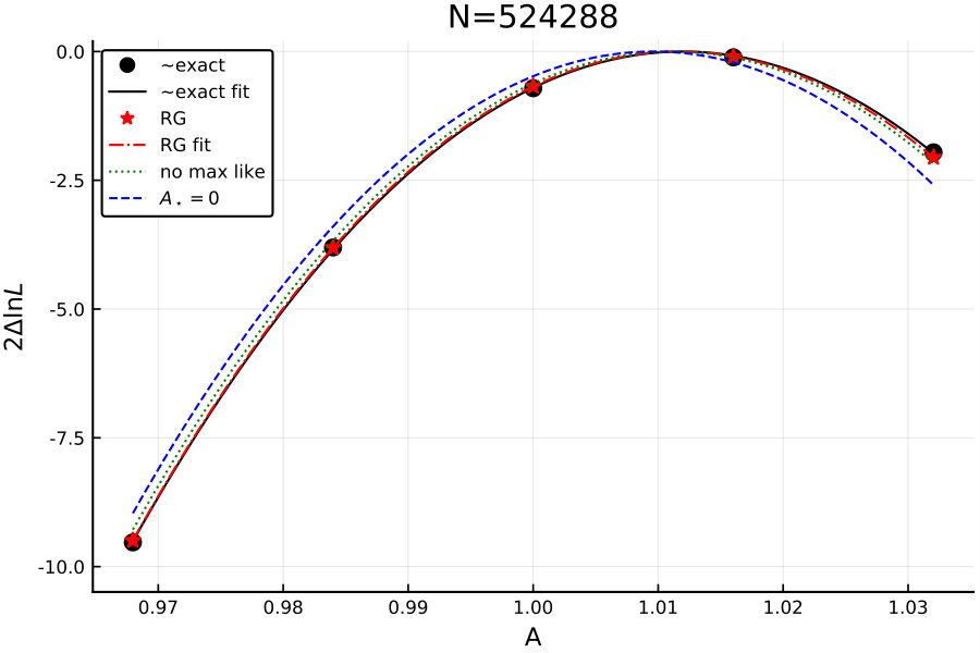 Figure 1
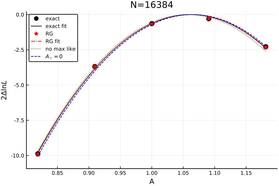 Figure 2
Peer Reviews
No public reviews on file for this paper yet. If you reviewed it on a platform where reviews are public (OpenReview, ICLR, NeurIPS, ICML), you can paste yours below so the community can read it here.
Videos
No videos yet. Explain this paper in a talk, walkthrough, or lecture? Add one.
Improved renormalization group computation of likelihood functions for
cosmological data sets
Patrick McDonald
Lawrence Berkeley National Laboratory, One Cyclotron Road, Berkeley, CA 94720, USA
Abstract
Evaluation of likelihood functions for cosmological large scale structure data sets (including CMB, galaxy redshift surveys, etc.) naturally involves marginalization, i.e., integration, over an unknown underlying random signal field. Recently, I showed how a renormalization group method can be used to carry out this integration efficiently by first integrating out the smallest scale structure, i.e., localized structure on the scale of differences between nearby data cells, then combining adjacent cells in a coarse graining step, then repeating this process over and over until all scales have been integrated. Here I extend the formulation in several ways in order to reduce the prefactor on the method’s linear scaling with data set size. The key improvement is showing how to integrate out the difference between specific adjacent cells before summing them in the coarse graining step, compared to the original formulation in which small-scale fluctuations were integrated more generally. I suggest some other improvements in details of the scheme, including showing how to perform the integration around a maximum likelihood estimate for the underlying random field. In the end, an accurate likelihood computation for a million-cell Gaussian test data set runs in two minutes on my laptop, with room for further optimization and straightforward parallelization.
I Introduction
McDonald (2019) presented a new method to evaluate large scale structure likelihood functions, inspired by renormalization group (RG) ideas from quantum field theory (e.g., Wilson and Kogut, 1974; Banks, 2008). This paper is a followup to that one, so some of the pedagogical discussion and derivations there will not be repeated here. To recap the basics: the fact that structure in the Universe starts as an almost perfectly Gaussian random field and evolves in a computable way on the largest scales (e.g., Peebles, 1993; McDonald and Roy, 2009; McDonald and Vlah, 2018) suggests a statistically rigorous first-principles likelihood analysis can be used to extract information on cosmological models from observational data sets (e.g., Bond et al., 1998; Wandelt et al., 2004; Kitaura and Enßlin, 2008; Enßlin et al., 2009; Enßlin, 2019). Generally, we have a data vector , some relatively small number of global cosmological parameters we want to measure, , and a random field we’d like to marginalize over, . ( could be a variety of different things, depending on the data set and theoretical setup, e.g., the underlying true temperature field for CMB, the linear regime density and/or potential fields for a galaxy redshift survey modeled by traditional perturbation theory, the evolving displacement field in the functional integral formulation of McDonald and Vlah (2018), etc.) Starting with Bayes’ rule we obtain
[TABLE]
where I have dropped which has no parameter dependence and the prior which plays no role in this discussion because it can be pulled out of the integral. I have highlighted the usual cosmological form where some of the cosmological parameters determine a prior on the signal field, , and then there is some likelihood for the observable given and , . It is this integral that we need to carry out. Generally, we can take at least part of , , to be Gaussian, defined by its covariance, . In this case we have
[TABLE]
where I have used and defined . (Even for what we call non-Gaussian initial conditions (e.g., McDonald, 2008; Bartolo et al., 2010; Giannantonio and Porciani, 2010; Gong and Yokoyama, 2011; Alvarez et al., 2014; Moradinezhad Dizgah and Dvorkin, 2018), the observable can often if not always be written as a function of an underlying Gaussian random field, i.e., no needed, and in other scenarios like McDonald and Vlah (2018) where the natural is not Gaussian, there is still a natural Gaussian piece.) Less generally but still often usefully (e.g., for primary CMB and large scale galaxy clustering ignoring primordial non-Gaussianity) we can take and to be Gaussian by assuming is linearly related to , i.e., where is the mean vector, is a linear response matrix, and is Gaussian observational noise with covariance matrix . Then we have
[TABLE]
where in the last line the integration has been carried out analytically, with . Even this analytic integration does not really solve the Gaussian problem, however, as the time to calculate and (or its derivatives) by brute force numerical linear algebra routines scales like , where is the size of the data set, which becomes prohibitively slow for large data sets. The RG approach of McDonald (2019) addresses the Gaussian scenario by doing the integral in a different way that produces the result directly as a number instead of these matrix expressions, and can also be applied to non-Gaussian scenarios. Note that, as discussed in McDonald (2019), the approach can also be used to directly compute derivatives of with respect to , not just the value at one choice of , by passing the derivative inside the integral to produce a new integral. Traditional power spectrum estimation can be done by taking to parameterize by amplitudes in bands.
In spite of the fact that fairly fast methods to evaluate at least the Gaussian likelihood [Eq. (I)] have existed for a long time (e.g., Pen, 2003; Padmanabhan et al., 2003; Smith et al., 2007; Seljak et al., 2017; Font-Ribera et al., 2018), more often in practice data analysts compute summary statistics not explicitly based on likelihood functions (e.g., Aghanim et al., 2016; Beutler et al., 2017), calibrating their parameter dependence and covariance by computing the same statistics on mock data sets. It is not entirely clear why existing likelihood-based methods are not used more often, and in McDonald (2019) I was cautious about advocating immediate implementation of the RG approach. One question was if the prefactor on the linear scaling of computation time with data set size for this method might be so large as to make it significantly slower than others. This paper demonstrates that this is not a significant obstacle. At two minutes to accurately compute the likelihood function for a million-cell Gaussian test data set, the method is as fast as any that takes more than a few well-preconditioned conjugate gradient maximum likelihood solutions for the same data set (i.e., as fast as any method I know of, barring the possibility that my Julia implementation of conjugate gradient maximum likelihood is unfairly slow). The only reason not to implement this is if you believe the whole idea of likelihood-based analysis is a distraction. That would not necessarily be an entirely unreasonable position. E.g., if you believe that there is a lot of reliable cosmological constraining power to be gained from the deeply non-linear regime, heuristic summary statistics/“machine learning,” combined with exhaustive mocks/simulations is probably the only way to extract it. To me, however, the likelihood+RG approach proposed here seems like an appealing path to large scale analysis, especially for incorporating weakly nonlinear information (e.g., without the need to explicitly estimate a bispectrum and its covariance).
This paper lays out a series of essentially technical improvements to the basic approach presented in McDonald (2019). See that paper for a derivation of the general RG equation and some more pedagogical discussion. Some of that basics are explained in less detail here when they can be read there.
II Revised formulation
II.1 Master RG equation
Consider the general functional integral over some field ,
[TABLE]
The connection to our cosmological likelihood functions, Eq. (2), is obvious, but not necessary for this subsection. Suppose that , i.e., goes to infinity (all its eigenvalues). In that limit the part of becomes a representation of the delta function and it is clear that , i.e., the integral can be done trivially. Generally, however, is not sufficiently small so if we want to do the integral this way we need to change to take it to zero. But we can’t simply change because that will change the value of , the integral we are trying to perform. If we want to change while preserving we need to simultaneously change . The renormalization group equation tells us how to do this. Guided by, e.g., Banks (2008), McDonald (2019) showed that we can preserve the value of if the following differential equation is satisfied:
[TABLE]
where we parameterize the evolution by , i.e., , , and the prime means derivative with respect to , where and represent the original elements of the integral. (Note that, relative to Eq. (7) of McDonald (2019), I have moved the normalization constant into , after extracting from it to keep the integral unit normalized when .) This formula is pure math, i.e., it assumes essentially nothing about , , and . Typically will represent a length scale, where structure in has already been erased on smaller scales, and is doing the job of erasing it on scale , but Eq. (5) applies to any infinitesimal change in .
II.2 Application to Gaussian cosmological data
As in McDonald (2019), I will demonstrate the calculation for a purely Gaussian example, i.e., at most quadratic in . This is a special case only—Eq. (5) applies for any . The likelihood function will be Eq. (I), except for simplicity I will set , i.e., I take
[TABLE]
For the RG method to be efficient, the linear response matrix and the observational noise cannot be completely arbitrary. Ideally should be fairly short range, e.g., a CMB telescope beam convolution or redshift space cells in which we have counted galaxies. Similarly, should be short-range, e.g., diagonal for uncorrelated noise. The general approach can be adapted for special kinds of deviations from short range or , but I will assume they are short range here. I generally assume the problem can be formulated to make translation invariant (i.e., diagonal in Fourier space), although slow evolution in statistics can easily be accommodated. It is potentially useful to change integration variables to , where is some constant field specified by hand. We plan to make the maximum likelihood field, but do not need to assume that. Substituting this into Eq. (6) and comparing to Eq. (4), understanding that in Eq. (4) is a dummy variable so we can just as well replace it with , we see that the general integral in Eq. (4) is equivalent to the the Gaussian cosmological if we define
[TABLE]
and
[TABLE]
The reason for subtracting from and adding it to the term (adding zero overall, with an as yet unspecified matrix) will become clear below.
As in McDonald (2019), the evolving Gaussian is represented numerically by the evolving coefficients , , and of the general form
[TABLE]
Comparison to Eq. (II.2) for sets the initial conditions for , , and :
[TABLE]
[TABLE]
and
[TABLE]
Plugging Eq. (9) into Eq. (5) we find the flow equations for , , and :
[TABLE]
[TABLE]
[TABLE]
Note that if is the maximum likelihood field (for given values of , , etc.), . If the problem happened to be statistically homogeneous (translation invariant), we could set to make . In that case there would be no evolution— would simply be the answer. This is the point of , i.e., if we choose it to be as close as possible to , we can reduce the RG evolution to be a minimal correction due to statistical inhomogeneities. The limitation, i.e., why generally can only approximate , is that must maintain the symmetries necessary to allow us to efficiently evaluate in Eq. (12), e.g., in Fourier space, to set the initial value of .
In terms of these definitions, the result of formal analytic integration is
[TABLE]
We can use this formula once the components have been coarse-grained sufficiently to allow brute force linear algebra. To be clear: if we plug , , , and into this equation, it becomes precisely the analytic integration result in Eq. (I) (with ). The difference is that as these quantities evolve and are coarse grained their dimensions become smaller, with the result of the small-scale integration that has been performed stored in the simple number . See McDonald (2019) for more discussion.
II.3 Integrating out the difference between adjacent cells
In McDonald (2019) I used
[TABLE]
where to suppress fluctuations. I mentioned the potentially cleaner possibility
[TABLE]
where , e.g., . Either of these was envisioned to suppress fluctuations in a smooth, homogeneous way (i.e., with no explicit connection to the data cell structure), starting from small scales to large. Once fluctuations were sufficiently suppressed on the scale of data cells, adjacent cells were combined, i.e., adjacent elements in and the corresponding block in were summed. This worked well enough, but the number of elements that I needed to store in , which determines the speed of computation, seemed surprisingly large.
Here I introduce a new possibility, to more explicitly integrate out the fluctuations between pairs of cells that we are going to combine (see Appendix A for an alternative version of this idea). Given covariance matrix for some vector, we know that the covariance for a new vector where each adjacent pair of elements is replaced by one element with its average, , is simply given by the average of the appropriate blocks of , e.g., , , etc. This makes clear that if we define , where is the matrix of equivalent dimension to but with the blocks that will be compressed to replaced by their average (e.g., ), we can straightforwardly evolve Eq. (5) from a starting to ending , followed by a coarse graining combination of cells, and repeat. Formally, for each iteration what we are doing is defining so that , and solving the differential equation (5) for running from 0 [where ] to 1 [where ].
The obvious problem here is that generally is a dense matrix, which we can’t have if the method is to be fast. The key to the RG approach working is that elements of will generally be small very far off-diagonal, i.e., physically we do not expect the correlation at wide separations to change much when the separation is changed by a small fractional amount. To put it another way, we do not expect to need to use small cells when measuring correlations at wide separations. This allows us to drop most elements of , keeping it, and as influenced by it, sparse. The closest thing to an exception to this “no fine structure at large separations” rule that comes to mind is the BAO feature—a relatively narrow bump at wide separation. Considering such a thing, we observe that it is only necessary for to remain sparse, not strictly near-diagonal, i.e., we can if necessary include a strip of elements somewhere off-diagonal in , propagate this into , etc., as long as there are not too many of these elements.
Operationally, this program is surprisingly straightforward. I start by computing one full row of . This is basically just a standard computation of a correlation function given a power spectrum, i.e., this matrix obeys translation invariance by construction, so its elements are a function only of separation, inverses can be done in Fourier space, and one row is all that is necessary to capture the full matrix. This becomes described above and I compute the first two rows of (the block-averaged matrix) directly from it. From this I compute the full sparse including only elements above some threshold. I define the threshold to be some fraction of the maximum absolute value of , called , i.e., I keep elements with . Note that this makes no assumption about the structure of , e.g., an off-diagonal stripe due to something like BAO will be propagated if it passes the threshold.
After evolving , , and through Eqs. (13)-(15), they, along with as represented by a single row, are coarse-grained by factors of two (i.e., elements summed in the case of and and averaged in the case of ) and the next iteration proceeds exactly as before. All of the problem-specific details go into the construction of , , , and —after that the algorithm proceeds essentially identically for any problem. After enough iterations the effective data set becomes small enough to finish the calculation by brute force using the analytic integral formula, Eq. (16).
Note that, while my test problems will be one dimensional, where factors of two coarse graining by combining adjacent pixels is the obvious thing to do, there is no obvious reason not to do this as well in higher dimensions. On a cartesian grid we can combine adjacent cells in one direction at a time. On a sphere, a hiearchical block of four HEALPixels Górski et al. (2002) can be combined in two steps of pair combinations. However, it should also be possible to generalize the method to combine more than two cells at a time. as discussed above just needs to represent the appropriately averaged covariance.
II.4 Sparsification
While the cut discussed above limits the range in somewhat, in practice I find that the evolution of produces many small elements that do not need to be fully propagated for accuracy and slow down the calculation significantly. In McDonald (2019) I maintained the sparsity of by computing elements only out to some maximum separation, taken to be a multiple of the RG distance scale . Here I suggest a potentially more generally adaptive method, along the lines of the element size cut discussed above involving . The key equation numerically is Eq. (13), because the matrix products there dominate the computation time. To control this, I introduce two more numerical parameters. When evaluating , I first trim using another threshold parameter, , again basing the cut on the absolute value of elements relative to the maximum absolute value. To be clear, I am not permanently dropping part of the stored, evolving , only the matrix used to compute . I apply another similar cut defined by to , before using it to update in each step. In practice, for simplicity, I only use one of these two cuts at a time, finding the cut to be slightly more efficient in my test problems.
II.5 Numerical demonstration
For numerical tests I use one dimensional scenarios similar to McDonald (2019). I use signal power spectrum with or , where is measured in units of the data cell size. I add unit variance noise to each cell. I generate mock data with and calculate likelihoods as a function of . I use pivot so that the case has both signal and noise dominated ranges of scales. To be sure the test covers both fine structure and edges, I create statistically inhomogeneous data sets where the rms noise level in every fourth cell is multiplied by a factor of 10, and the noise in the last quarter of the data vector is similarly multiplied.
It is more difficult to make a non-trivial test with the innovations in this paper, because if I assume periodic data with homogeneous noise so that I can compute the exact likelihood to compare to using FFTs, the obvious choice of sets so the RG evolution is almost trivial. If I also find the maximum likelihood field to use for , so that , it is completely trivial. For this reason I only do tests with inhomogeneous data in this paper, first on data sets small enough to compute the exact likelihood by brute force linear algebra, demonstrating that the RG method works precisely in the appropriate limit of the numerical parameters, then with large data sets where the truth is determined by using much better than necessary values for numerical parameters.
After some experimentation, my standard numerical parameter settings are as follows: is set to , where is the noise power in the good part of the data—this sets the accumulated term in Eq. (15) to approximately zero (the results are insensitive to the exact value of , as long as it is reasonable). I specify the number of mid-point method steps per factor of two coarse graining by a numerical parameter . My standard setting is (in an advanced version of the method, one could try to apply all the usual tricks for solving differential equations numerically). I set , and .
II.5.1 Small problems
I first do some tests with , where we can still pretty quickly compute the exact likelihood by brute force linear algebra, shown in Fig. 1.
The results are good, by construction of course. Both using a maximum likelihood and using to remove the mean effect of from the evolution improve the accuracy at fixed parameter settings, although for these settings (which were driven by larger data sets) the difference is not critical. This example has , which is generally a little more difficult for the algorithm than .
II.5.2 Large problems
If we are convinced that the algorithm works in the sense of producing accurate results in the appropriate limit of numerical parameters, we can do non-trivial large-scale tests by simply looking for convergence as the numerical parameters are changed, i.e., we assume that if there is convergence it is to the correct result. Figure 2 shows an test, for again.
The results are again excellent. One might guess based on these figures that my numerical parameter settings are too conservative, i.e., that I could loosen them to achieve better speed. This is not actually true—there seems to be some cancelation of errors that makes the results in these particular examples so perfect, and they go bad very quickly if the parameters are loosened.
I stop at for these examples because careful testing on my laptop becomes tedious beyond this, especially running with extremely conservative parameter settings to be certain of the exact result. I have run up to two million cells with good looking results. A one million cell example runs in two minutes. At four million I start to exhaust the memory on my laptop in my current Julia implementation, although it would be possible to go somewhat further with more optimization. In any case, it is clear that billion cell data sets could be done comfortably on a supercomputer.
I tried evolving using , more like in McDonald (2019), but with a maximum likelihood , , and element size cuts as introduced in this paper, but was unable to come within a factor of ten of the performance of the pairwise suppression approach of this paper.
III Discussion
To summarize, I have suggested the following improvements to the basic RG approach of McDonald (2019):
- •
Integrating out the difference between cells that are to be combined, rather than small-scale structure more generally, by defining directly to be proportional to the difference between the current and target covariance.
- •
Shifting integration variables to integrate around a maximum likelihood signal field, if available, as .
- •
Subtracting a statistically homogeneous approximation out of the numerically evolving matrix , through the definition of .
- •
Cuts on matrix element size, specified by , , etc., instead of a simple range cut.
The first of these is by far the most important. In the end it is clear that the algorithm is fast and straightforward enough for convenient practical data analysis.
It was surprising to me that the pair-oriented definition of made such a large (factor ) difference in speed. While the the principle that if we know which cells we will combine we should focus on integrating out the difference between them seems good enough to expect some improvement, I would have been happy with a factor of two. It may be that I do not have the best possible implementation of the smooth cutoff option. In any case though, it seems like the pair-oriented approach is the way to go.
Of course it is only useful to integrate around a maximum likelihood field if that field can be found more quickly than the RG analysis could be done without it. This was the case in my tests, where finding the maximum likelihood field by conjugate gradient (CG) takes about 5% of the time in each likelihood computation. This might not always be the ratio, as my CG solution was massively accelerated by being able to multiply by things like in Fourier space, including for preconditioning (e.g., without preconditioning finding a maximum likelihood field takes longer than the RG integration without it). If, e.g., the CG had to be done using less efficient spherical harmonic transforms, it might be faster not to use it. An interesting possibility is to use the RG method itself to find the maximum likelihood field. McDonald (2019) showed how to find the data-constrained mean of any function of , with itself being the simplest possible version of this. For a Gaussian problem is the maximum likelihood field, while for a non-Gaussian problem it is not but would probably be a better starting point than the maximum likelihood field in that case anyway. Finding can be piggybacked on a standard likelihood computation with minimal extra cost, but to get a speedup in likelihood calculations you would need to feed the result back into a recalculation. This would only be effective if a useful estimate of could be found with looser numerical settings than would be required to do the calculation with , which seems quite possible. When, e.g., computing derivatives with respect to parameters, we would probably achieve most of the benefit by computing only for the central model (remember that accurate results can be achieved for any , it is just a question of how tight numerical settings need to be to do it).
Note that it may not always be beneficial to use . There is no cost if all cells in a formal data vector have measurements, i.e., there are no zeros on the diagonal of , but if a substantial number of cells represent large holes in the data set or zero padding, so that these elements of can be dropped from sparse storage, setting will remove this possibility. This must be considered on a problem-by-problem basis.
While my prototype code is already quite fast, at two minutes per likelihood evaluation per million cells, there is clearly more room for optimization. Most obviously, I am not taking advantage of the fact that and are symmetric matrices at all, for no better reason than not knowing canned operations in Julia that will do this. Other simple improvements could be tuning of things like the cuts I’ve parameterized by , etc.. I kept these cuts constant for all iterations but this could be wasteful if the required cut value is set by coarser levels of the calculation that do not take much total time. A less obvious but I think promising optimization idea is the following: The effect of evolving Eq. (13) is non-linear in the matrix as initial changes in are multiplied back together to find the next step, i.e., we get products of with itself. The required number of steps is surely set by the products of the largest elements of —the products of small elements are perturbatively much smaller. This suggests that could be split into two or more pieces based on element size. The piece(s) with larger elements, which would be very short-range (i.e., few elements, i.e., fast to multiply), could be evolved first, then longer-range the pieces with smaller elements evolved with fewer steps, possibly even one, because their self-products are negligible. As long as our set of steps integrates to , we are free to choose the details.
The next step is to implement this for realistic cosmological scenarios.
Acknowledgements.
I thank Zack Slepian and Uroš Seljak for helpful comments. This work was supported by the U.S. Department of Energy, Office of Science, Office of High Energy Physics, under Contract No. DE-AC02-05-CH11231.
Appendix A Alternative approach to integrating out differences between cells
Before realizing I could define by simply differencing the current and target s, I worked out a method for integrating out the difference between cells closer to the original approach in McDonald (2019). I include it here to promote broader understanding of the possibilities.
The RG integration will be controlled by a parameter which starts at zero and is taken to . and become functions of this parameter, i.e.,
[TABLE]
with a fixed matrix to be specified. Obviously we can suppress fluctuations between cells 1 and 2 by adding a term to proportional to . Repeating this over and over (e.g., , etc.) is equivalent to making the following block diagonal matrix:
[TABLE]
where
[TABLE]
I.e., by dialing from 0 to in , we will have effectively integrated out the differences between adjacent pairs of cells. We now have
[TABLE]
Unlike in McDonald (2019), is not exactly translation invariant, so we can’t simply compute in Fourier space. The structure of is the same everywhere, however, up to a distinction between odd and even cells, and it is limited to short range, so we can compute it by brute force inversion for a limited representative stretch of cells and then translate it everywhere.
This approach worked in preliminary tests, but not as efficiently as the one in the paper.
The reference list from the paper itself. Each links out to its DOI / PubMed record.
- 1Mc Donald (2019) Patrick Mc Donald, “Renormalization group computation of likelihood functions for cosmological data sets,” Phys. Rev. D 99 , 043538 (2019) . · doi ↗
- 2Wilson and Kogut (1974) K. G. Wilson and J. Kogut, “The renormalization group and the ϵ italic-ϵ \epsilon expansion,” Phys. Rept. 12 , 75–199 (1974) . · doi ↗
- 3Banks (2008) T. Banks, Modern Quantum Field Theory, by Tom Banks, Cambridge, UK: Cambridge University Press, 2008 (2008).
- 4Peebles (1993) P. J. E. Peebles, Principles of Physical Cosmology by P.J.E. Peebles. Princeton University Press, 1993. ISBN: 978-0-691-01933-8 (1993).
- 5Mc Donald and Roy (2009) P. Mc Donald and A. Roy, “Clustering of dark matter tracers: generalizing bias for the coming era of precision LSS,” JCAP 8 , 020 (2009) , ar Xiv:0902.0991 [astro-ph.CO] . · doi ↗
- 6Mc Donald and Vlah (2018) Patrick Mc Donald and Zvonimir Vlah, “Large-scale structure perturbation theory without losing stream crossing,” Phys. Rev. D 97 , 023508 (2018) . · doi ↗
- 7Bond et al. (1998) J. R. Bond, A. H. Jaffe, and L. Knox, “Estimating the power spectrum of the cosmic microwave background,” Phys. Rev. D 57 , 2117–2137 (1998).
- 8Wandelt et al. (2004) Benjamin D. Wandelt, David L. Larson, and Arun Lakshminarayanan, “Global, exact cosmic microwave background data analysis using Gibbs sampling,” Phys. Rev. D 70 , 083511 (2004) , ar Xiv:astro-ph/0310080 [astro-ph] . · doi ↗