Restart FISTA with Global Linear Convergence
Teodoro Alamo, Pablo Krupa, Daniel Limon

TL;DR
This paper introduces a new restart scheme for FISTA that guarantees global linear convergence in non-strongly convex problems satisfying quadratic growth, without needing prior knowledge of certain parameters.
Contribution
The paper proposes a novel restart scheme for FISTA that achieves global linear convergence without requiring prior parameter knowledge.
Findings
Outperforms existing restart FISTA schemes in simulations
Achieves global linear convergence for non-strongly convex problems
Does not require prior knowledge of the objective's optimal value or growth parameter
Abstract
Fast Iterative Shrinking-Threshold Algorithm (FISTA) is a popular fast gradient descent method (FGM) in the field of large scale convex optimization problems. However, it can exhibit undesirable periodic oscillatory behaviour in some applications that slows its convergence. Restart schemes seek to improve the convergence of FGM algorithms by suppressing the oscillatory behaviour. Recently, a restart scheme for FGM has been proposed that provides linear convergence for non strongly convex optimization problems that satisfy a quadratic functional growth condition. However, the proposed algorithm requires prior knowledge of the optimal value of the objective function or of the quadratic functional growth parameter. In this paper we present a restart scheme for FISTA algorithm, with global linear convergence, for non strongly convex optimization problems that satisfy the quadratic growth…
Click any figure to enlarge with its caption.
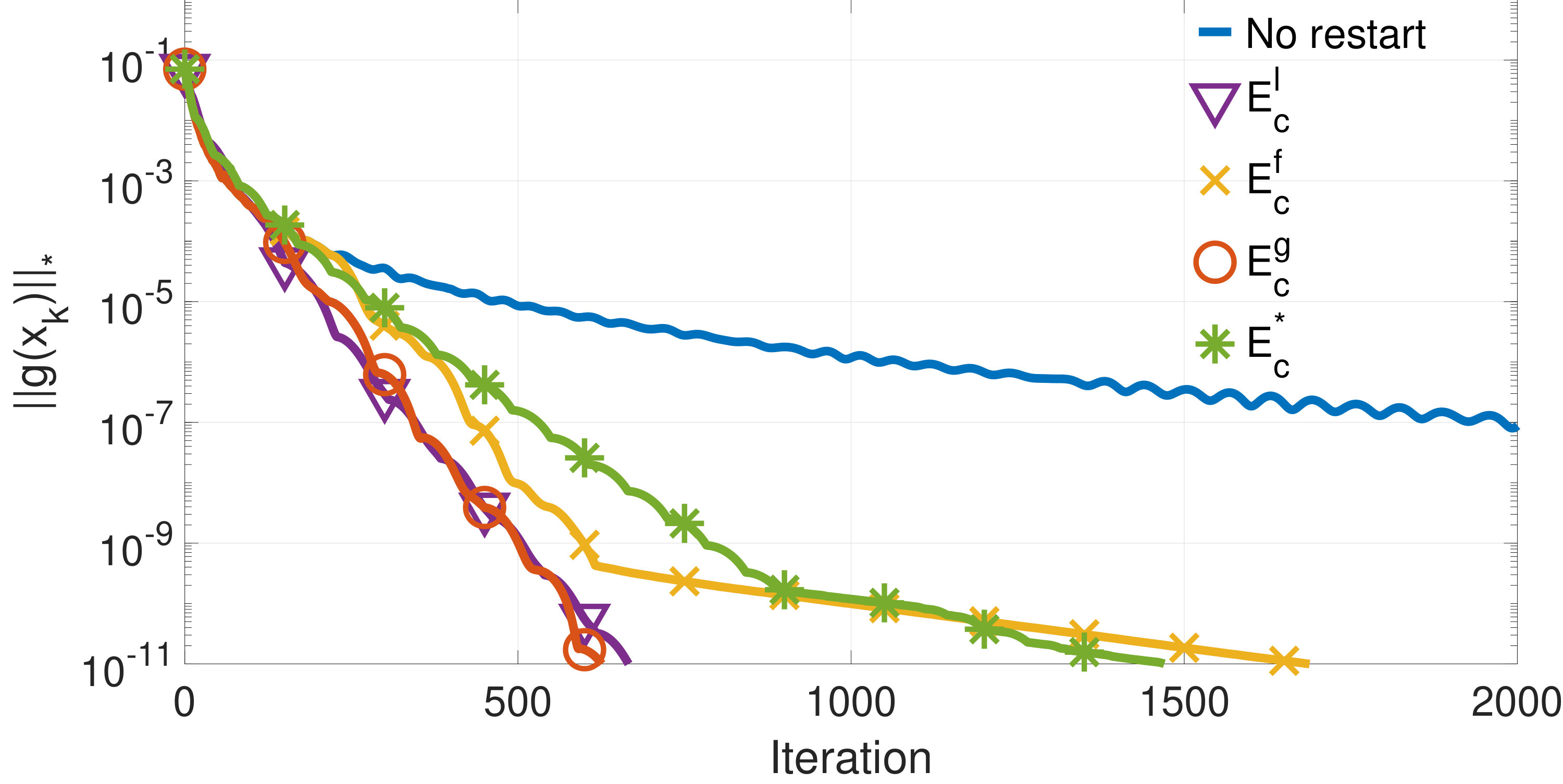 Figure 1
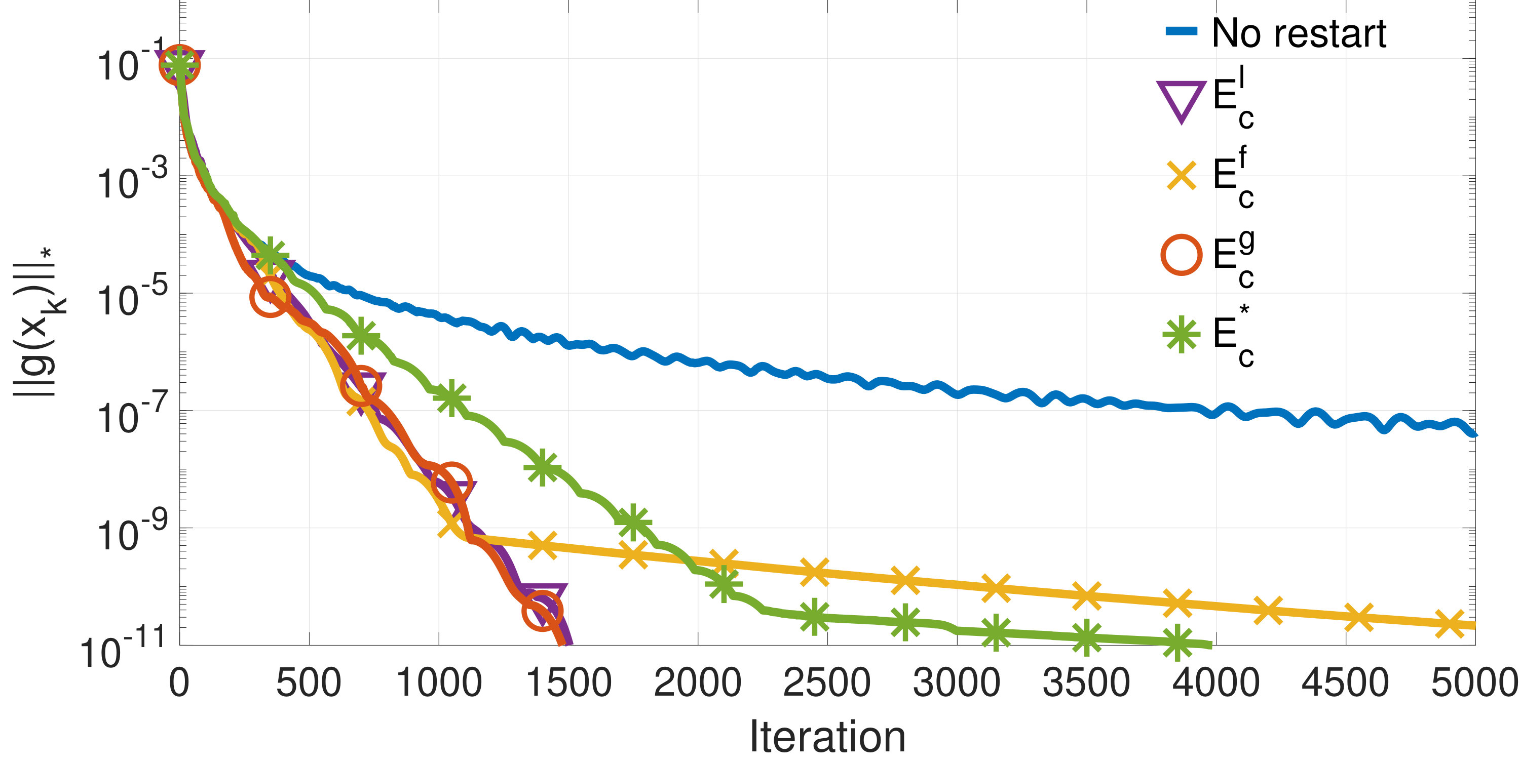 Figure 2
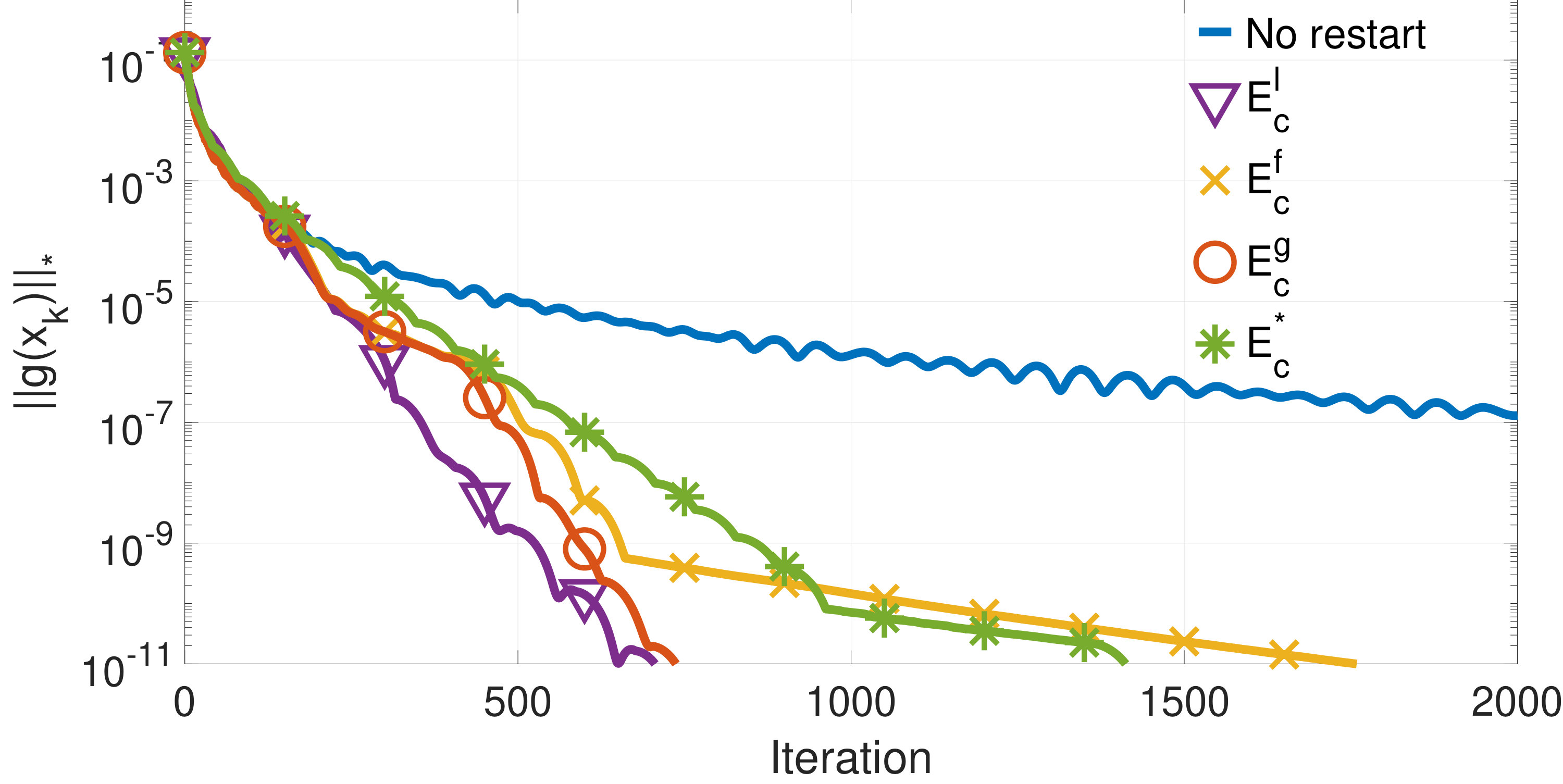 Figure 3
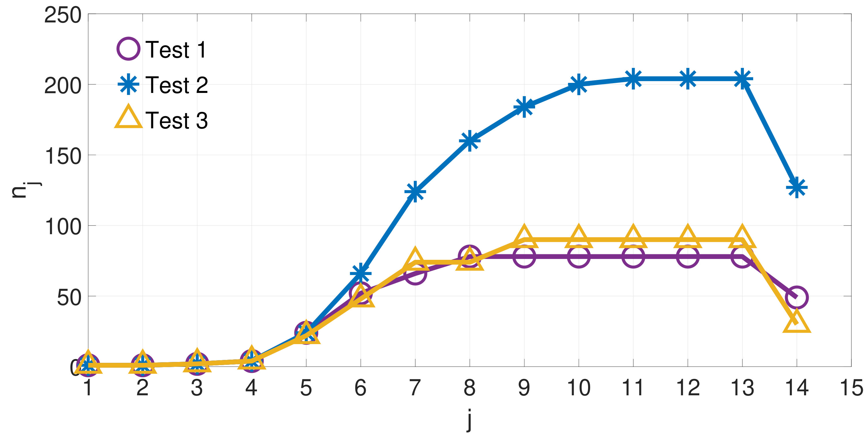 Figure 4
| Exit Cond. | No restart | ||||
|---|---|---|---|---|---|
| Avg. Iter. | |||||
| Median Iter. | |||||
| Max. Iter. | |||||
| Min. Iter. |
| Exit Cond. | No restart | ||||
|---|---|---|---|---|---|
| Avg. Iter. | |||||
| Median Iter. | |||||
| Max. Iter. | |||||
| Min. Iter. |
| Exit Cond. | No restart | ||||
|---|---|---|---|---|---|
| Avg. Iter. | |||||
| Median Iter. | |||||
| Max. Iter. | |||||
| Min. Iter. |
Peer Reviews
No public reviews on file for this paper yet. If you reviewed it on a platform where reviews are public (OpenReview, ICLR, NeurIPS, ICML), you can paste yours below so the community can read it here.
Videos
No videos yet. Explain this paper in a talk, walkthrough, or lecture? Add one.
Restart FISTA with Global Linear Convergence
Teodoro Alamo, Pablo Krupa and Daniel Limon T. Alamo, P. Krupa and D. Limon are at the Systems Engineering and Automation Department, University of Seville, Spain. E-mail: {talamo,pkrupa,dlm}@us.esThe authors acknowledge MINERCO and FEDER funds for funding project DPI2016-76493-C3-1-R, and MCIU and FSE for the FPI-2017 grant. This paper constitutes an extended and revised version of [1]. Some of the technical results presented in this paper are used in [2].
Abstract
Fast Iterative Shrinking-Threshold Algorithm (FISTA) is a popular fast gradient descent method (FGM) in the field of large scale convex optimization problems. However, it can exhibit undesirable periodic oscillatory behaviour in some applications that slows its convergence. Restart schemes seek to improve the convergence of FGM algorithms by suppressing the oscillatory behaviour. Recently, a restart scheme for FGM has been proposed that provides linear convergence for non strongly convex optimization problems that satisfy a quadratic functional growth condition. However, the proposed algorithm requires prior knowledge of the optimal value of the objective function or of the quadratic functional growth parameter. In this paper we present a restart scheme for FISTA algorithm, with global linear convergence, for non strongly convex optimization problems that satisfy the quadratic growth condition without requiring the aforementioned values. We present some numerical simulations that suggest that the proposed approach outperforms other restart FISTA schemes.
Keywords
Fast gradient method, restart FISTA, convex optimization, linear convergence, quadratic functional growth condition.
I Introduction
Fast gradient methods (FGM) were introduced by Yurii Nesterov in [3], [4], where it was shown that these methods provide a convergence rate O for smooth convex optimization problems with non strongly convex objective functions [4], where is the iteration counter. These methods were generalized to composite non smooth convex optimization problems in [5], [6], [7]. The resulting algorithm is commonly known as FISTA algorithm [5]. Because of its complexity certification, it is often used in the context of embedded model predictive control [8], [9], [10]. Another possibility to address composite convex optimization problems is to use splitting methods like ADMM [11], [12], [13].
FISTA algorithms can be applied in a primal setting (as in the Lasso problem [5]), or in a dual one [14], [15]. They can be thought of as a momentum method, since the linearization point at each iteration depends on the previous iterations. Since the momentum grows with the iteration counter, the algorithm can exhibit undesirable periodic oscillating behavior for certain applications, which slows the convergence rate. To mitigate this, restart schemes have been proposed in the literature which stop the algorithm when a certain criteria is met. It is then restarted using the last value provided by the stopped algorithm as the new initial condition [16], [17], [18].
In [16] two heuristic restart schemes for FGM are proposed which exhibit improved convergence rates over non-restart FGM schemes. These restart schemes reset the momentum of the FGM in order to eliminate the undesirable oscillations whenever the periodical behavior is detected. A restart scheme similar to the ones in [16] with O convergence rate for smooth convex optimization is presented in [18]. In [19], an algorithm is proposed that uses the restart schemes from [16]. Numerical results show improvements over previous restart schemes for FGM, but no theoretical results on convergence rates are provided.
Recently, linear convergence rate has been derived for several first order methods applied to convex optimization problems with non strongly convex objective functions that satisfy a relaxation of the strong convexity known as the quadratic functional growth [20].
In [20, Subsection 5.2.2] a restarting scheme of FGM is presented with global linear convergence rate for convex optimization problems that satisfy the functional growth condition with parameter . However, in order to implement this strategy, prior knowledge is needed of either the optimal value of the objective function or the value of , which can be challenging to compute.
In this paper we propose a novel restart scheme for FISTA algorithm applied to solving convex constrained problems. We show that the algorithm guarantees global linear convergence rate O for convex optimization problems with non strongly convex objective functions that satisfy the quadratic functional growth condition with parameter . The proposed algorithm does not require prior knowledge of the value of or of the optimal value of the objective function. We provide theoretical upper bounds on the number of iterations of the algorithm needed to achieve a given accuracy.
Additionally, we show numerical results comparing the proposed algorithm with the heuristic restart schemes from [16] and the restart scheme from [20] for Lasso problems.
In Section II we introduce the problem formulation. Section III presents FISTA algorithm and some restart schemes. The convergence rate of non restart FISTA algorithm under the satisfaction of the quadratic functional growth condition is presented in Section IV. In Section V we present the proposed restart scheme for FISTA and state its global linear convergence. Numerical results comparing the proposed algorithm with other restart schemes applied to FISTA are shown in Section VI. Finally, conclusions are presented in Section VII.
Notation
Given vectors and , we denote by their scalar product, i.e. . Given vector , denotes its Euclidean norm (), and denotes its -norm (sum of the absolute values of the components of ). Given we denote by the weighted Euclidean norm , and by its dual norm. is the natural logarithm and is Euler’s number. denotes the largest integer smaller than or equal to ; denotes the smallest integer greater than or equal to . Given a set we denote by its indicator function. That is, if , and if . The relative interior of set is denoted by . Given the extended real valued function we denote by its effective domain. That is, . We denote by the epigraph of . That is, . We say that function is closed if its epigraph is a closed set. We say that is proper if its effective domain is not empty. That is, if is not identically equal to . We say that a vector is a subgradient of at a point if , . The set of all subgradients of at is called the subdifferential of at and is denoted by .
II Problem Formulation
We address the problem of solving the composite convex minimization problem
[TABLE]
under the following assumption.
Assumption 1**.**
We assume that
- (i)
* is a smooth differentiable convex function. That is, there is such that the inequality*
[TABLE]
is satisfied for every and . 2. (ii)
* is a closed convex function and is a closed convex set.* 3. (iii)
Denote . The minimization problem
[TABLE]
is solvable. That is, there is such that .
We notice that it is standard to write down the first point of Assumption 1 as
[TABLE]
where parameter serves to characterize the smoothness of and is a positive definite matrix. Constant provides a bound on the Lipschitz constant of the gradient [4, Subsection 2.1]. Since
[TABLE]
we have that (3) implies (2) if we take . This simplifies the algebraic expressions needed to analyze the convergence of the proposed algorithm.
We notice that Assumption 1 guarantees that the minimization problem (1) is solvable. The optimal set is defined as
[TABLE]
This set is a singleton if is strictly convex. Given we will denote its closest element in the optimal set (with respect to the norm ). That is,
[TABLE]
Given , one could use the local information given by to minimize the value of around . Under Assumption 1, this can be done obtaining the minimizer of the strictly convex optimization problem
[TABLE]
It is well known that this problem is solvable and has a unique solution if Assumption 1 holds (see, for example, Subsection 6.1 in [21] for an analogous result). For completeness we provide a proof of this statement in Appendix -A (see Property 5).
The solution to this optimization problem leads to the notion of composite gradient mapping [6], which constitutes a generalization of the gradient mapping that can be found in [4, Subsection 2.2] for the particular case . See also [5] for the particular case .
Definition 1** (Composite Gradient Mapping ).**
Under Assumption 1, and given , we define
[TABLE]
We notice that the composite gradient mapping is closely related to the notion of proximal operator [22], [21, Chapter 6]. For example, one could state, after some manipulations, the computation of the composite gradient mapping as the computation of a proximal operator. In the context of optimal gradient methods, it is assumed that the computation of is cheap. This is the case when is a simple set (box, , etc.), diagonal, and a separable function. For example, in the well known Lasso optimization problem, the computation of resorts to the computation of the shrinkage operator [5]. See [23], Section 6 of [22], Chapter 28 in [24], or Chapter 6 in [21], for numerous examples in which the computation of the composite gradient mapping is simple.
The following property gathers well-known properties of the composite gradient mapping and its dual norm [5], [6]. For completeness, we include the proof in Appendix -B.
Property 1**.**
Suppose that Assumption 1 holds. Then,
- (i)
For every and :
[TABLE] 2. (ii)
For every :
[TABLE]
The composite gradient serves to characterize optimality [6]. That is, under Assumption 1 we have the following equivalence
[TABLE]
This fact is proved in Appendix -C.
III Restart FISTA Schemes
For a given initial condition , a minimum number of iterations , and an exit condition , the non restart FISTA algorithm [5] is shown in Algorithm 1. This algorithm solves under Assumption 1.
Since the optimality of is equivalent to (see Property 7 in Appendix -C), a typical choice for non restart FISTA schemes is to choose equal to zero and codify the exit condition
[TABLE]
where is an accuracy parameter. It is also common to use the exit condition , since this exit condition requires , which has already been computed in step 1 of the algorithm.
It is well known that under Assumption 1, see also (3), the iterations of non-restart FISTA satisfy [5, 6],
[TABLE]
where represents the point in the optimal set closest to the initial condition of the algorithm (see (4)). For the sake of completeness, we present a detailed proof of this claim in Appendix -D. We also prove in the same appendix that the sequence generated by Algorithm 1 (FISTA) satisfies
[TABLE]
In restart schemes, one invokes several times FISTA algorithm with a relaxed exit condition. Typical choices are (see [16]),
- (i)
Function scheme:
[TABLE] 2. (ii)
Gradient scheme:
[TABLE]
Given initial condition , a minimum number of iterations , an exit condition , and an accuracy parameter , the standard restart FISTA algorithm is shown in Algorithm 2.
The implementation of Algorithm 2 usually provides better performance than the original non restart version [16], [18].
IV Convergence of Restart FISTA under a quadratic functional growth condition
It has been recently shown in [20] that some relaxations of the strong convexity conditions of the objective function are sufficient for obtaining linear convergence for several first order methods. In particular, the following relaxation of strong convexity suffices to guarantee linear convergence of different gradient optimization schemes for smooth functions (). See [20, Subsection 5.2.2].
Assumption 2** (Quadratic Functional Growth).**
We assume that the optimization problem
[TABLE]
is solvable and satisfies the following quadratic functional growth condition with parameter :
[TABLE]
where denotes the closest element to in the optimal set (see (4)).
As can be seen in [20, Subsection 3.4], strong convexity implies quadratic functional growth. This means that the quadratic functional growth setting encompasses a broad family of convex functions.
It is also shown in [20, Subsection 5.2.2] that if the value of is known and , then a restart FISTA based on the exit condition
[TABLE]
exhibits global linear convergence. This exit condition is easily implementable if the optimal value is known. This is the case, for example, in some formulations of feasibility optimization problems, in which the optimal value is equal to zero for every feasible solution. This restart scheme corresponds to an optimal restart rate of [20, Subsection 5.2.2].
We present now a novel result that further characterizes the convergence properties of the non restart FISTA algorithm under Assumption 2.
Property 2**.**
Under Assumptions 1 and 2, the iterations of FISTA algorithm satisfy
- (i)
, for all . 2. (ii)
, for all . 3. (iii)
, for all .
Proof.
See Appendix -F.
V Restart FISTA with global linear convergence
In this section we propose a novel restart FISTA algorithm (Algorithm 3) that exhibits global linear convergence under the quadratic functional growth condition. The algorithm uses exit condition , which is defined to be true if the following two conditions are satisfied,
[TABLE]
with .
Inequality (9b) guarantees that the output of the FISTA algorithm is no larger than the one corresponding to its initial condition.
As it is stated in the following property, one of the main features of the proposed algorithm is that the number of iterations required at each FISTA iteration is upper bounded by . Moreover, the number of iterations required by the proposed algorithm to attain a given accuracy is upper bounded by
[TABLE]
Property 3**.**
Suppose that Assumptions 1 and 2 hold. Then, the sequences , provided by Algorithm 3 satisfy
- (i)
, . 2. (ii)
, . 3. (iii)
The number of iterations () required to guarantee is no larger than
[TABLE]
Proof.
See Appendix -G.
We notice that the factor 16 in the worst case complexity analysis is conservative. The authors claim that a better factor might be obtained at the expense of a more involved proof.
VI Numerical results
We consider a weighted Lasso problem of the form
[TABLE]
where , is sparse with an average of of its entries being zero (sparsity was generated by setting a probability for each element of the matrix to be [math]), , and . Each nonzero element in and is obtained from a Gaussian distribution with zero mean and covariance 1. is a diagonal matrix with elements obtained from a uniform distribution on the interval .
We note that Lasso problems (9j) can be reformulated in such a way that they satisfy the quadratic growth condition [20, Section 6.3]. For this problem, inequality (2) of Assumption 1 is satisfied, for instance, for a matrix chosen as
[TABLE]
with . This is due to the Gershgorin Circle Theorem [25, Subsection 7.2]. See also [6, Section 6].
We show the results of applying algorithms 2 and 3 with an accuracy parameter using different restart schemes and values of , and . We take .
The restart schemes shown are (6) and (7) from [16], restart condition (8) [20], and the restart condition (9) proposed in this paper (using Algorithm 3). Additionally, we show the results of applying FISTA algorithm without using a restart scheme. In order to provide a fair comparison between the performance of the restart schemes, the algorithms are exited as soon as a value of that satisfies is found. We note that, in order to implement the restart scheme based on , we had to previously compute the optimal value , which was done by using Algorithm 3 with .
Tables I to III show results of performing tests with different randomized problems (9j) that share common values of parameters , and . Tables show the average, median, maximum and minimum number of iterations.
Figures 1 to 3 show the value of for a randomly selected problem out of the randomized problems used to compute the results shown in tables I to III, respectively.
Figure 4 shows the value of at each iteration of Algorithm 3 for the three examples whose results are shown in Figures 1 to 3. Note that the final value of is lower than the previous one in all three instances due to the algorithm exiting as soon as the condition is satisfied.
VII Conclusions
In this paper we have presented a novel restart scheme with guaranteed global linear convergence. The algorithm relies on a quadratic functional growth condition. One of the advantages of the proposed algorithm is that it does not require the knowledge of the parameter that characterizes the quadratic functional growth condition, or the optimal value of the minimization problem. We provide an upper bound of the required number of iterations equal to
[TABLE]
We have presented numerical evidence of the good performance of the algorithm when compared with other restarts schemes. It outperforms the restart scheme based on the knowledge of the optimal value .
-A Existence and Uniqueness of Composite Gradient
We present in this appendix some well known facts about convex analysis that are required to analyze the properties of the composite gradient.
Property 4**.**
Suppose that
- (i)
* is a closed convex function.* 2. (ii)
* is a closed convex set.* 3. (iii)
The set is non empty. 4. (iv)
* is the indicator function of . That is,*
[TABLE] 5. (v)
The function is defined as
[TABLE]
Then
- (i)
The function is proper, closed, and convex. 2. (ii)
The relative interior of is non empty. 3. (iii)
There is and such that and
[TABLE]
Proof.
From we have that both and are non empty. The epigraph of the indicator function is, by definition,
[TABLE]
Since and are non empty closed sets, is also a non empty closed convex set. Thus, by definition, is a closed convex function. Since both and are closed convex functions, is also a closed convex function (the sum of closed convex functions provides closed convex functions [26, Proposition 1.1.5]). Since , we infer that the domain of is non empty. This implies that is not identically equal to . Moreover, since we have that . We conclude that for every . From this and the fact that is not identically equal to we have that is proper.
Since is a non empty convex set, it has a non empty relative interior (see [26, Proposition 1.3.2]).
It is a well know fact from convex analysis that the subdifferential of a proper convex function at a point in the relative interior of its domain is non empty [26, Proposition 5.4.1]. Suppose now that . Since is a proper convex function we have that the subdifferential of at is non empty. This means, by definition, that there is such that
[TABLE]
∎
Property 5**.**
Suppose that Assumption 1 holds. Given any , consider the quadratic function defined as
[TABLE]
Then, the minimization problem
[TABLE]
is solvable and has a unique solution. That is, there exists a unique point such that
[TABLE]
Proof.
Notice that the minimization problem (9k) is equivalent to
[TABLE]
where is the indicator function of . If we define we can rewrite the original problem (9k) as
[TABLE]
We notice that the assumptions of Property 4 are satisfied if Assumption 1 holds. Thus, we infer from Property 4 that is a proper closed convex function. We also have that the quadratic function is also proper and closed because it is a real valued continuous function (see [26, Proposition 1.1.3]). Since the sum of closed functions is closed (see [26, Proposition 1.1.5]), we infer that is a closed function. Moreover, from Property 4 we also have that there is and such that
- (i)
. 2. (ii)
, .
Therefore,
[TABLE]
We infer from (9l) that the closed function is not identically equal to and therefore, proper. We conclude that is a proper closed convex function. From Weiertrasss’ Theorem (see Proposition 3.2.1 in [26]) we have that the set of minima of over is nonempty and compact if there is a scalar such that the level set is nonempty and bounded. From (9l) we have that is nonempty. Moreover, we also infer from (9l) that is a bounded set because is lower bounded by a strictly convex quadratic function of . We conclude that
[TABLE]
is a solvable optimization problem. That is, there is such that
[TABLE]
The set of minimizers consists of a single element because of the strictly convex nature of ( is a strictly convex function). ∎
-B Proof of Property 1.
We prove in this appendix Property 1, which is rewritten here for the reader’s convenience.
Property 6**.**
Suppose that Assumption 1 holds. Then,
- (i)
For every and :
[TABLE] 2. (ii)
For every :
[TABLE]
Proof.
From Property 5 we have that there is a (unique) such that
[TABLE]
where . Denote now , where is the indicator function of . Since we have . Therefore, inequality (9n) implies
[TABLE]
Denote now . From last inequality we have
[TABLE]
By definition of subdifferential at a point, we have that the previous inequality implies
[TABLE]
We have that is a proper closed function and (see the first two claims of Property 4). The domain of the quadratic function is . Since is a continuous real value function in , it is also closed (see Proposition 1.1.3 in [26]). We have that
[TABLE]
Since is equal to the sum of two closed convex functions and
[TABLE]
we have (see Proposition 5.4.6 in [26]). The subdifferential of the differentiable function at is . Thus, we obtain from (9o)
[TABLE]
Since is defined as we obtain
[TABLE]
By definition of we have
[TABLE]
Obviously, since , this implies
[TABLE]
Since and for every , we obtain
[TABLE]
The convexity of implies
[TABLE]
Adding this inequality to (9p) yields
[TABLE]
From Assumption 1 we have
[TABLE]
Adding this inequality to (9q) yields
[TABLE]
From this inequality we have
[TABLE]
This proves (9ma). We now prove (9mb) and (9mc) by means of simple algebraic manipulations.
[TABLE]
This proves (9mb). From this inequality, and the definition of , we obtain
[TABLE]
This proves (9mc). Suppose now that . Particularizing inequality (9r) to yields
[TABLE]
The inequality trivially follows from . ∎
-C Characterization of optimality
The following property serves to characterize the optimality of a given point .
Property 7**.**
Suppose that Assumption 1 holds. Then belongs to the optimal set
[TABLE]
if and only if .
Proof.
We first show that implies . Since , we infer from equality that is equivalent to . Suppose that . Then, we obtain from , , and the first claim of Property 1, the following inequality
[TABLE]
That is, . Since , this is possible only if is also optimal (). This proves that implies . We now prove that implies . Suppose that . Then, and we obtain from the second claim of Property 1
[TABLE]
This implies . ∎
-D *Convergence of non restart FISTA *
Property 8**.**
Suppose that Assumption 1 holds. Then, the sequences and generated by Algorithm 1 (FISTA) satisfy
- (i)
, for all , 2. (ii)
, for all ,
where represents the point in the optimal set closest to the initial condition of the algorithm.
Proof.
First claim:
We denote , . Additionally, we recall that .
From step 4 of FISTA algorithm we have
[TABLE]
This implies that
[TABLE]
Particularizing inequality (9mc) of the first claim of Property 6 to , and , we obtain
[TABLE]
By construction we have that and . Furthermore, by definition of , we have . Therefore we can rewrite previous inequality as
[TABLE]
This proves the claim of the property for . We now proceed to prove the claim for . From equality (9s) we have
[TABLE]
Therefore, from inequality (9mb) of Property 6 we obtain that for every and every
[TABLE]
We notice that, by construction, , . Particularizing at and , we obtain from last inequality
[TABLE]
In order to write down the proof in a compact way, we introduce the following incremental notation, valid for all ,
[TABLE]
Inequalities (9ua) and (9ub) in an incremental notation, are
[TABLE]
We introduce now the auxiliary variable , defined as
[TABLE]
From Property 9 in appendix -E we have
[TABLE]
We now use this identity to obtain
[TABLE]
In view of Property 9, , . This implies that we can replace, in inequality (9w), and by the lower bounds given by inequalities (9va) and (9vb). In this way we obtain
[TABLE]
From step 6 of the algorithm we have for all that . This can be rewritten in incremental notation as
[TABLE]
We now define, for every
[TABLE]
From the definition of and (9y) we obtain
[TABLE]
[TABLE]
Using (9z) and (9aa) we now show that can be written in terms of and .
[TABLE]
With this expression for we obtain from (9ab)
[TABLE]
Thus, for every ,
[TABLE]
Equivalently
[TABLE]
Since this inequality holds for every we can apply it in a recursive way to obtain
[TABLE]
From (9t) we have
[TABLE]
Thus,
[TABLE]
Therefore,
[TABLE]
From this inequality, and taking now into account that for all (second claim of Property 9), we conclude
[TABLE]
That is,
[TABLE]
∎
Second claim:
We first prove the claim for .
[TABLE]
From (9t) we derive
[TABLE]
Thus,
[TABLE]
We now prove the claim for . From (9ad) we also have
[TABLE]
We also have that
[TABLE]
From (9ae) we derive . From this and (9af) we obtain
[TABLE]
From here we derive, for every ,
[TABLE]
From (9ac) we have
[TABLE]
Therefore, for every
[TABLE]
We notice that the last inequality is due to the second claim of Property 9. This proves the second claim of the property. ∎
-E Properties of the sequence
Property 9**.**
Let us suppose that and that
[TABLE]
Then
- (i)
, for all . 2. (ii)
, for all .
Proof.
- (i)
For every , is defined as one of the roots of
[TABLE]
Therefore we obtain . 2. (ii)
The claim is trivially satisfied for equal to 0. We now show that if the claim is satisfied for then it is also satisfied for .
[TABLE]
Since the claim is assumed to be satisfied for we have and consequently
[TABLE]
∎
-F Proof of Property 2
From equation (5) we have
[TABLE]
Due to Assumption 2 we also have
[TABLE]
Therefore,
[TABLE]
This proves the first claim. Denote
[TABLE]
With this notation we rewrite (9ai) as
[TABLE]
Suppose now that . Then,
[TABLE]
Therefore,
[TABLE]
This, along with inequality (9aj), yields
[TABLE]
Equivalently,
[TABLE]
This proves the second claim of the property. In view of inequality (9aj) we have
[TABLE]
Therefore,
[TABLE]
Suppose now that . This implies and consequently (see (9ak)). Dividing both terms of inequality (9al) by , we get
[TABLE]
∎
-G Proof of Property 3
By construction, , for all . Therefore, we have from the second claim of Property 1, that
[TABLE]
We also notice that is computed invoking FISTA algorithm using as initial condition (). That is,
[TABLE]
Since the output value is forced to be no larger than the one corresponding to , we have . Therefore, we obtain from inequality (9am) that
[TABLE]
This proves the first claim of the property. We now show that if , then the value obtained from
[TABLE]
also satisfies
[TABLE]
Denote
[TABLE]
Since , we infer, from the third claim of Property 2, that
[TABLE]
From this inequality, we obtain
[TABLE]
Therefore, the first exit condition is satisfied for . Since we have . This means that for , the corresponding value for is no larger than
[TABLE]
We also notice that, in view of the second claim of Property 2, the additional exit condition is satisfied for every
[TABLE]
Therefore, implies that , obtained from , also satisfies (9an). We now prove, by reduction to the absurd, that cannot be larger than . Suppose that
[TABLE]
Because of the previous discussion, the previous inequality could be forced only by the doubling step of the algorithm. That is, inequality (9ao) is possible only if there is such that and
[TABLE]
Since
[TABLE]
we have that is obtained from applying
[TABLE]
iterations of FISTA algorithm. However, we have from the third claim of Property 2 that this number of iterations implies
[TABLE]
From the second claim of Property 1 we also have . Thus,
[TABLE]
That is, there is no doubling step if . This proves the second claim of the property.
We now show that there is a doubling step at least every
[TABLE]
steps of the algorithm. Suppose that there is no doubling step from iteration to , where . That is,
[TABLE]
From this, and the first claim of the property, we obtain the following sequence of inequalities
[TABLE]
We conclude that consecutive iterations without doubling step implies that the exit condition is satisfied (). We conclude that there must be at least one doubling step every iterations. This implies that there exist such that
[TABLE]
Therefore, . Moreover, since is a non decreasing sequence, we get , . That is,
[TABLE]
Suppose that is rewritten as , where and . From the non decreasing nature of ,
[TABLE]
Also, from inequality (9ap), we have . Using this inequality in a recursive manner we obtain
[TABLE]
This, allows us to infer from (9aq) that
[TABLE]
The last claim of the property follows directly from this one and the bound of the second claim. That is, if denotes the first index for which , we get that the number of total iterations is bounded by
[TABLE]
∎
The reference list from the paper itself. Each links out to its DOI / PubMed record.
- 1[1] T. Alamo, P. Krupa, and D. Limon, “Restart FISTA with global linear convergence,” in 2019 18th European Control Conference (ECC) . IEEE, 2019, pp. 1969–1974.
- 2[2] ——, “Gradient based restart FISTA,” in Proceedings of the 58th IEEE Conference on Decision and Control (CDC) . IEEE, 2019, pp. 3936–3941.
- 3[3] Y. Nesterov, “A method of solving a convex programming problem with convergence rate O ( 1 / k 2 ) 1 superscript 𝑘 2 (1/k^{2}) ,” Sov. Math. Dokl. , vol. 27, no. 2, pp. 372–376, 1983.
- 4[4] ——, Introductory Lectures on Convex Optimization: A Basic Course . Springer, 2004.
- 5[5] A. Beck and M. Teboulle, “A fast iterative shrinkage-thresholding algorithm for linear inverse problems,” SIAM J. Imaging Sciences , vol. 2, no. 1, pp. 183–202, 2009.
- 6[6] Y. Nesterov, “Gradient methods for minimizing composite functions,” Mathematical Programming , vol. 140, pp. 125–161, 2013.
- 7[7] P. Tseng, “On accelerated proximal gradient methods for convex-concave optimization,” Dept. Math., Univ. Washington, Seattle, WA, USA, Tech. Rep., 2008.
- 8[8] M. Kögel and R. Findeisen, “A fast gradient method for embedded linear predictive control,” in 18th IFAC World Congress , 2011, pp. 1362–1367.