Hybrid Planning for Dynamic Multimodal Stochastic Shortest Paths
Shushman Choudhury, Mykel J. Kochenderfer

TL;DR
This paper introduces DMSSPs, a new class of MDPs for complex decision-making under uncertainty, and proposes HSP, a hybrid algorithm that improves planning efficiency and solution quality in dynamic multimodal environments.
Contribution
The paper presents a novel class of MDPs called DMSSPs and a hybrid planning algorithm HSP that combines heuristic search, approximate dynamic programming, and hierarchical planning.
Findings
HSP outperforms state-of-the-art algorithms in autonomous multimodal routing.
HSP achieves higher quality solutions with efficient computation.
The approach effectively handles uncertainty and dynamic updates in complex environments.
Abstract
Sequential decision problems in applications such as manipulation in warehouses, multi-step meal preparation, and routing in autonomous vehicle networks often involve reasoning about uncertainty, planning over discrete modes as well as continuous states, and reacting to dynamic updates. To formalize such problems generally, we introduce a class of Markov Decision Processes (MDPs) called Dynamic Multimodal Stochastic Shortest Paths (DMSSPs). Much of the work in these domains solves deterministic variants, which can yield poor results when the uncertainty has downstream effects. We develop a Hybrid Stochastic Planning (HSP) algorithm, which uses domain-agnostic abstractions to efficiently unify heuristic search for planning over discrete modes, approximate dynamic programming for stochastic planning over continuous states, and hierarchical interleaved planning and execution. In the domain…
Click any figure to enlarge with its caption.
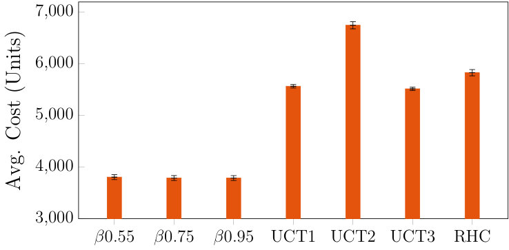 Figure 1
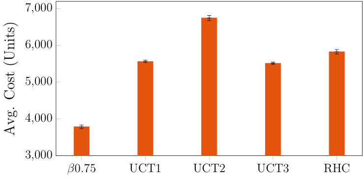 Figure 2
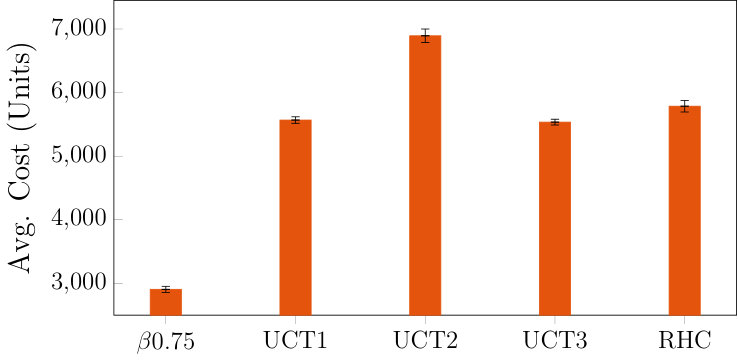 Figure 3
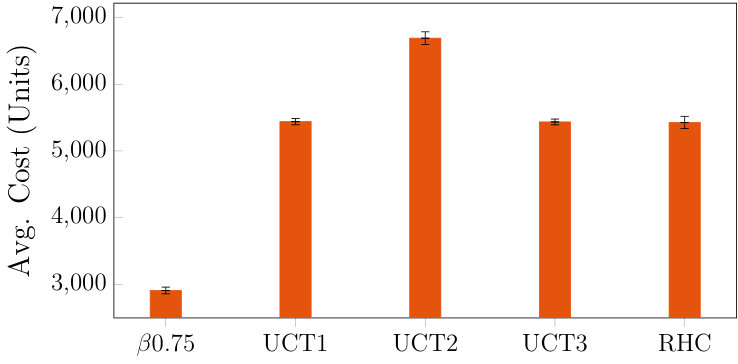 Figure 4
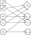 Figure 5
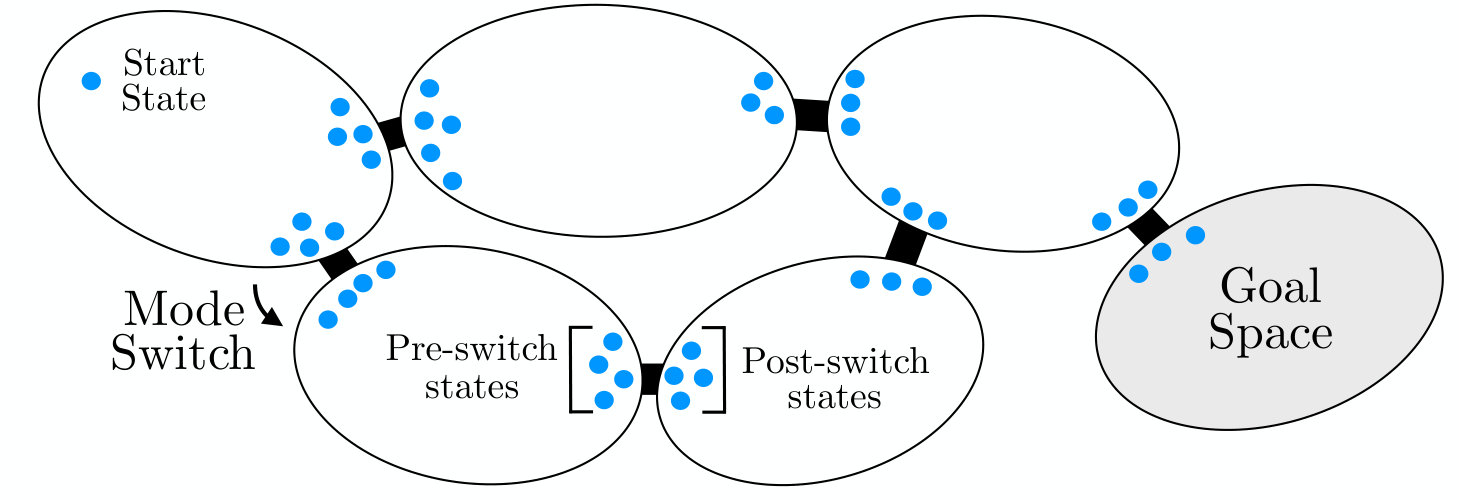 Figure 6
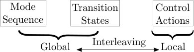 Figure 7
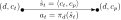 Figure 8
 Figure 9
| Variant | depth | exploration | n_iterations | init_N |
|---|---|---|---|---|
| UCT1 | ||||
| UCT2 | ||||
| UCT3 |
| Episode Set | Num. Routes | Perturbation Prob. |
|---|---|---|
| Set 1 (in main) | ||
| Set 2 | ||
| Set 3 |
| Algorithm | Set 1 | Set 2 | Set 3 |
|---|---|---|---|
| (HSP) | |||
| UCT1 | |||
| UCT2 | |||
| UCT3 | |||
| RHC |
| Algorithm | Avg. Time () |
|---|---|
| HSP Global Layer | |
| HSP Local Layer | |
| UCT1 | |
| UCT2 | |
| UCT3 | |
| RHC Global Layer | |
| RHC Local Layer |
Peer Reviews
No public reviews on file for this paper yet. If you reviewed it on a platform where reviews are public (OpenReview, ICLR, NeurIPS, ICML), you can paste yours below so the community can read it here.
Code & Models
Videos
No videos yet. Explain this paper in a talk, walkthrough, or lecture? Add one.
Taxonomy
TopicsAI-based Problem Solving and Planning · Robotic Path Planning Algorithms · Multi-Agent Systems and Negotiation
Hybrid Planning for Dynamic
Multimodal Stochastic Shortest Paths
Shushman Choudhury
Department of Computer Science
Stanford University
&Mykel J. Kochenderfer
Department of Aeronautics and Astronautics
Stanford University
Abstract
Sequential decision problems in applications such as manipulation in warehouses, multi-step meal preparation, and routing in autonomous vehicle networks often involve reasoning about uncertainty, planning over discrete modes as well as continuous states, and reacting to dynamic updates. To formalize such problems generally, we introduce a class of Markov Decision Processes (MDPs) called Dynamic Multimodal Stochastic Shortest Paths (DMSSPs). Much of the work in these domains solves deterministic variants, which can yield poor results when the uncertainty has downstream effects. We develop a Hybrid Stochastic Planning (HSP) algorithm, which uses domain-agnostic abstractions to efficiently unify heuristic search for planning over discrete modes, approximate dynamic programming for stochastic planning over continuous states, and hierarchical interleaved planning and execution. In the domain of autonomous multimodal routing, HSP obtains significantly higher quality solutions than a state-of-the-art Upper Confidence Trees algorithm and a two-level Receding Horizon Control algorithm.
1 Introduction
Consider the problem of a robot arm picking and arranging objects from a conveyor belt. This simple example captures several challenges of sequential decision-making for robotics: (i) the system state is a hybrid of discrete logical modes (is the robot holding an object or not) and continuous robot state values (joint angles); (ii) external information that constrains the inter-modal transitions (the object positions that define where they can be picked up) is dynamically changing; (iii) the objective is to reach a goal (a given arrangement) with minimum cumulative trajectory cost, i.e. a stochastic shortest paths problem [1], which is challenging because the cost of a solution depends on both the high-level sequence of objects grasped and the underlying motor control actions. We define a class of Markov Decision Processes with the above properties, which we call the Dynamic Multimodal Stochastic Shortest Path (DMSSP) problem. DMSSPs can represent many general decision-making problems of importance in robotics, such as task and motion planning for mobile manipulation [2, 3] and autonomous multimodal routing [4].
Work on such robotics planning problems (hybrid state space, uncertainty, online information, solution quality as the objective) have largely focused on efficiently solving deterministic variants, delegating management of uncertainty to a low-level controller and replanning when it fails. For a time-constrained setting, however, uncertainty in the dynamics may have significant downstream effects, e.g. not reaching an object in time may invalidate the plan and greatly increase cost. A framework that accounts for uncertainty in a high level plan will be more robust to anticipating and avoiding downstream errors and temporal constraint violations. We are motivated by designing such a framework while mitigating the inevitable increase in complexity due to considering uncertainty.
Existing planning algorithms for solving large MDPs, which do account for uncertainty, would encounter several hurdles with DMSSPs. For offline MDP methods based on value or policy iteration, even with hierarchical decomposition [5] and state-of-the-art function approximators [6], it is typically infeasible to generate a good policy over the entire space of external information. Online MDP methods based on stochastic tree search suffer from the large depth and branching factor for long-horizon search over continuous states and discrete modes.
Our work builds upon the idea that a principled composition of classical search-based planning, planning for MDPs, and hierarchical planning can reason over long horizons, explicitly account for the underlying uncertainty, and replan efficiently online. We develop an algorithmic framework with three broad components: a global open-loop layer that plans for a sequence of discrete modes, a local closed-loop layer that controls the agent under uncertainty through the modes, and hierarchical interleaved planning and execution to adapt to dynamic external information. We expect the resulting approach to achieve better quality solutions on DMSSPs than existing MDP methods.
Our contributions are as follows: (i) We introduce and formulate the problem of Dynamic Multimodal SSPs. (ii) We design a Hybrid Stochastic Planning algorithm for decision-making in DMSSPs, which uses a careful choice of domain-independent representations and abstractions to efficiently incorporate heuristic search, approximate dynamic programming, and hierarchical interleaved planning and execution. (iii) We demonstrate how our approach outperforms two complementary baselines—a state-of-the-art Upper Confidence Trees algorithm and a two-level Receding Horizon Control algorithm—on real-time multimodal routing problems.
Related Work Overview
We provide a brief summary of the concepts we build upon. Our formulation is based on Markov Decision Processes (MDPs) [7] and Stochastic Shortest Paths [1], an undiscounted goal-directed negative-reward MDP. Our DMSSPs model share elements with previously studied MDP models: arbitrarily modulated transition functions [8], stochastic shortest paths with online information [9], and factored hybrid-space MDPs [10]. Our HSP algorithm uses ideas from heuristic search [11, 12] and search-based planning for multi-step tasks [13, 14], approximate dynamic programming [15, 6], hierarchical planning for solving large MDPs [16, 17, 18], and interleaved planning and execution [19, 20]. A body of relevant previous work incorporates heuristic search and classical AI techniques in algorithms for solving MDPs [21, 22, 23]. Several works from the robotics planning community solve related problems using local information to inform global planning and trajectory optimization [24, 25] and explore various aspects of combined (discrete) task and (continuous) motion planning [3, 2] such as planner-agnostic abstractions [26], stochastic shortest path formulations [27, 28], and hierarchical planning and execution [29, 30]. Our optimization-based formulation is similar to that for Logic-Geometric Programming [31].
2 Dynamic Multimodal Stochastic Shortest Paths (DMSSPs)
A DMSSP is a discrete-time MDP, . The state space is multimodal, i.e. factored as . Each represents a discrete logical mode of the system and is the continuous state space of the decision-making agent. The current system state is accordingly denoted as . The action space is where is the set of discrete mode-switching actions (e.g. Pickup and Putdown) and is the set of control actions for the agent. The context space is dynamic. At each time-step, the agent observes a discrete set of contexts . Here, is the current context and is the estimated context time-steps in the future. In general, . The context is assumed to be generated by an exogenous process whose evolution equation, i.e. , is complex and depends on a number of unobserved variables. The current context set is compactly denoted as . The set cardinality is some domain-dependent prediction horizon, and the dimensionality of context is time-varying, i.e. may differ from . In our example, the context is the current and estimated future positions of all moving objects on the belt.
The transition function can be factored as follows:
[TABLE]
The factored form efficiently encodes stochastic intra-modal physical dynamics in eq. 1a and context-dependent deterministic mode-switching rules in eq. 1b. We treat the discrete mode-switching as single time-step actions. The grounded values of logical predicates (for mode-switching) are represented as states [27], i.e. instances of and not just in eq. 1b. The current context restricts the actual grounding of the logical predicates in the preconditions and effects that define the mode switch rules. Precondition states need to be reached for a mode switch to be feasible and effect states are obtained after the mode switch is completed. In our running example, whether the end-effector can satisfy the preconditions to grasp a moving object depends on the end-effector (state space) and the object (context). As in typical stochastic shortest paths [1], the problem is episodic and undiscounted. Also, the reward function is non-positive, so we will also use ‘cost’ to represent negative rewards. It is factored in terms of the intra-modal costs, i.e. . The decision diagram of a DMSSP is depicted in fig. 1(a).
We explicitly write out a DMSSP as an online stochastic optimal control problem. Given a start state and goal space , the overall problem is:
[TABLE]
where is the number of steps taken. From fig. 1(b), a DMSSP planning algorithm has to choose a sequence of modes from start mode to goal mode , and also control the agent to traverse through the corresponding subspaces. Even the one-shot deterministic problem is a discrete-time Logic-Geometric Program [31], for which a globally optimal solution is infeasible. Theoretical optimality analysis requires several assumptions and is not our focus (additional comments in appendix A). We are interested in high quality solutions that are efficient.
3 Hybrid Stochastic Planning (HSP)
The challenges with DMSSPs preclude directly applying existing techniques for large MDPs, as mentioned in section 1. We develop a Hybrid Stochastic Planning framework that is particularly suited for DMSSPs. A global layer computes a sequence of mode switches and corresponding transition states; planning open-loop enables efficiently searching over long-horizon mode sequences. A local layer executes actions that control the agent within each mode; closed-loop planning provides some robustness to uncertainty. Additional hierarchical logic for interleaving planning and execution reacts to the dynamically changing context at both global and local levels. Figure 2 depicts a schematic of the HSP structure. The concepts we rely on have been studied extensively. However, what we particularly contribute are the design choices in the overall framework (discussed subsequently); heuristic search over mode sequences, decomposition to smaller MDPs, using cost-to-go functions, i.e. negative value functions as edge weight surrogates, pre-empting the local controller. These choices unite techniques from classical search-based planning, planning for MDPs, and hierarchical planning in a principled manner. Since DMSSP is a class of problems, we present a general algorithmic framework that can accommodate a variety of modular techniques and subroutines.
3.1 Global Open-loop Layer
This layer repeatedly computes a high-level plan from the current state to a goal state . The current high-level plan (computed at current time ) is denoted as follows:
[TABLE]
where and the sequence of chosen modes is . For each planned mode switch , the sampled precondition is and effect is . For each mode, is a closed-loop policy that controls the agent through the region from the effect after the previous switch to the precondition before the next switch . GlobalPlan in Algorithm 1 outlines the global layer, which runs a heuristic search [11, 13] from the current state to compute a sequence of modes and transition states towards the goal space . We briefly discuss the subroutines.
For NextValidModes, we use the mode-switch rules and the current context set to identify possible next modes from . The specific implementation is domain-dependent. In our example, the robot can only execute Pickup on objects that will be reachable based on the current context set. The SampleTransition method generates grounded precondition and effect states for the proposed mode switch given the context set, using some domain-specific sampling procedure (the number of samples is a parameter). It also generates , a probability distribution over future time-steps at which the context will satisfy the mode transition preconditions. In our example, we could use work on sampling end-effector poses for grasping a given object [32] at various steps along the object’s expected future trajectory (defined by the context).
For EdgeWeight, consider its role in the overall solution. Each call to GlobalPlan returns a sequence of modes and transition states. Subsequent execution by the local layer can only optimize the trajectory locally. The edge weight function should therefore be a good surrogate of the expected cost to have any hope of a good overall solution. The cumulative intra-modal dynamics cost depends on the actual trajectory that will eventually be executed by the agent in that mode. Therefore, as a surrogate, we use the cost-to-go function of the policy for a local MDP corresponding to the mode, where the local MDP state is encoded in the edge (details explained in section 3.2):
[TABLE]
Here, is the horizon-dependent cost-to-go function for the local MDP of mode . We have presented the most general search formulation for the global layer. It can use many of the speedup techniques for heuristic search-based planning [14, 33] to improve efficiency. The heuristic function () in general is defined on ; additional comments on the heuristic are in appendix B.
3.2 Local Closed-loop Layer
The local closed-loop layer in HSP controls the agent in its current mode up to the chosen transition state for the next switch. The layer is ‘local’ because it is only provided information about the currently executing step of the current global plan , i.e. , where is the current mode of the agent. For each mode , we define a local target-directed MDP , where the first argument of the state is the current position, and the second is the target. The control space is . The and functions are derived from and , i.e.
[TABLE]
The Cartesian self-product is required in general because the policy must be able to control the agent between any two states in . However, for many spaces, a state can be encoded with relative state , where is a difference operator, and the target is always the ‘origin’ , i.e. the zero state. Many modes typically share dynamics, so the same policy can be reused [17]. For example, in our setting, the robot dynamics effectively depend only on if an object is currently grasped or not, which can be encoded with two modal dynamics functions.
**Finite-Horizon Value Iteration
**The local closed-loop policy has a dual role, controlling the agent with low cost within the mode to the transition state chosen by the global layer and satisfying the temporal constraints of the context for the next mode switch (). If it is too slow, the mode transition may fail, affecting the overall solution. On the other hand, controlling the agent as quickly as possible may be highly sub-optimal. To model this tradeoff, we use finite-horizon value iteration to obtain a horizon-dependent policy [15]. The finite-horizon value iteration requires a horizon limit (we use the context horizon ) and a terminal cost . For all local MDP states , we compute for ,
[TABLE]
where represents both cost-to-go and action-cost-to-go (Q function), with overloading (negative reward i.e. positive cost). The full cost-to-go function, compactly denoted as , can be used in eq. 4. As in the global layer, we require only a general framework for value iteration; any local or global approximation scheme [6] and other approximate dynamic programming [15] techniques could be used. The regional closed-loop policy , invoked during execution online, is based on obtained offline. For the current DMSSP state , context horizon distribution , and transition state (provided by the global layer), the control action chosen locally for is
[TABLE]
**Terminal Pseudo-Cost
**To incentivize the closed-loop policy to reach the target, we need a terminal penalty for states where the target is not reached at horizon 0, i.e. , for some domain-dependent distance metric. We need to be careful while choosing the terminal penalty or pseudo-cost due to the sub-optimality of hierarchical MDP planning [5, 18]. The penalty is not in the true cost function in eq. 2, so the higher it is set, the poorer is as a surrogate of the true cost, and the more (locally) sub-optimal is as a controller. An insufficiently high penalty, on the other hand, may lead to choosing lower-cost actions at the risk of being unable to reach the target within the context horizon. Consequently, the attempted mode switch may fail, forcing HSP to recompute a different mode sequence, leading to much poorer solutions (downstream effects of uncertainty).
We set the penalty as the maximum cost of any -length action sequence within the mode, i.e.
[TABLE]
The pseudo-cost is the smallest penalty that prioritizes the mode sequence. The value can be computed offline and then used in the finite-horizon value iteration. Further comments on the pseudo-cost and horizon limit are made in appendices A and C). LocalPreprocessing in algorithm 1 outlines the local layer; the policies obtained from pre-processing are used online.
An implicit assumption of ours is that the MDP for the agent dynamics can be solved reasonably. This assumption is not always valid, e.g. a complex underactuated system or an articulated manipulator. However, for many practical systems, framing and solving the control problem with MDPs has been successful [34], and finite-horizon versions of those controllers could also be used here.
3.3 Hierarchical Interleaved Planning and Execution
Interleaving planning and execution is an important property for real-time decision-making. Our HSP framework uses the simplification approach to interleaving [19]. The global layer simplifies the underlying intra-modal control problem by determinization and planning over multiple timesteps, and computes a solution in this simplified space. The local layer executes the plan provided by the global layer. We discuss two aspects of our interleaving, each occurring at one of the levels, either global replanning or local pre-emption. The full HSP framework is outlined in algorithm 2.
**Global Replanning
**HSP uses a combination of event-driven and periodic replanning [35]. The two events that trigger replans asynchronously are closed-loop pre-emption and failed mode-switch attempts. The current global plan is then invalidated and a new plan must be generated before execution can resume. With periodic replanning, the global layer computes a new global plan from the current state synchronously in the background, while the local layer executes the current plan. The duration of the replanning period is domain-dependent; but a domain-agnostic strategy is to replan immediately after the previous plan has finished computing. This updates the local layer’s next target every time-steps, where is the ratio between closed-loop and open-loop frequencies. Each time a global plan has been recomputed by the global layer, the next target of the local policy is immediately updated to the (potentially) new transition state for the next switch (fig. 3 illustrates this).
**Local Pre-emption
**Updates to can make it difficult to reach the chosen mode transition state in time (e.g. a target object suddenly speeds up). The periodic global replanning does account for this. However, the latency is time-steps. We have additional closed-loop pre-emption logic to reason about the next chosen mode switch at the higher frequency of the local layer. For each local MDP, we compute and store (during pre-processing) the worst cost-to-go for any state from each horizon value, i.e. . During the online execution of the local layer, if the agent is at a state from where reaching the goal in the remaining horizon is sufficiently unlikely, i.e.
[TABLE]
where is a risk parameter. The lower is set, the lower the risk we are willing to take that the agent can reach the next transition state in time. In addition to a higher frequency for reasoning about pre-emption, this logic provides a modifiable risk aversion.
4 Experiments: Multimodal Routing Domain
We use a different domain than our running example; the recently introduced Dynamic Real-time Multimodal Routing (DREAMR) problem [4]. We omit an elaborate description of the domain (see appendix E for more). The DREAMR problem requires planning and executing routes under uncertainty for an autonomous agent that can use multiple modes of transportation in a dynamic transit vehicle network. There are two discrete modes in the problem, Move for when the agent moves by itself and Ride for when the agent uses transport. The continuous state is the agent’s position and velocity. The mode-switching actions are Board and Alight, which switch Move to Ride and vice versa respectively. The noisy agent control actions are for acceleration in each direction. The agent is penalized for energy expended due to movement and waiting in place, and total elapsed time. The transit vehicle routes are the contextual information; at any time, the current context set comprises the current position and estimated future route (as a sequence of waypoints) of each active vehicle. The estimated time of arrival (ETA) for each subsequent waypoint is subjected with some probability to a bounded two-sided deviation at each timestep. Mode switches can only be made at transit waypoints. Additionally, the agent can only Board a vehicle if it is sufficiently close to the waypoint at the same time as the vehicle, and sufficiently slow. The dimensionality of the context space increases with the number of active route waypoints, and so is highly dynamic and very large (in the thousands). Though there are technically only two modes, in practice, the number of valid mode sequences to the goal is exponential in the number of transit vehicle routes.
4.1 Baselines: Upper Confidence Trees and Receding Horizon Control
We use two complementary baselines to evaluate the benefit of our solution. First, a (domain-specific) two-level Receding Horizon Control (RHC) method which repeatedly solves a deterministic problem. It uses graph search for planning routes, and non-linear receding horizon control trajectory optimization for executing them. The second is based on Upper Confidence Trees (UCT) [36], a general online MDP planning algorithm, with two enhancements: (i) techniques from PROST [37], a state-of-the-art UCT-based probabilistic planner [38]; (ii) double progressive widening [39] which artificially limits the branching factor and is more suitable for a continuous state space. We additionally assist the UCT baseline: (i) the value function estimates and Q-value initializations are informed by (ii) the tree depth is set to the same horizon limit as the HSP local layer (iii) many trials are run to compute good estimates for each action.
4.2 Results
We used the POMDPs.jl framework [40] in Julia (additional details in appendix D and attached code111The Julia code is at https://github.com/sisl/CMSSPs). For HSP, we chose three values for the risk parameter for attempting time-constrained risk parameters: , and (for lower values, it is overly risk-averse and rejects most transit connections). For UCT, we chose three different combinations of the number of virtual rollouts at a new tree node and the UCB exploration constant. The RHC does not have an important tuning parameter. We used the same large-scale problem scenarios as the original DREAMR paper (see appendix E for more details and parameter values). We evaluated each algorithm instantiation on simulated episodes. Figure 5 shows the average cumulative trajectory cost; both UCT and RHC produce poorer quality trajectories than HSP. Figure 5 displays the average number of executed mode switches. Appendix E.3 has average computation times, and performance results on two additional sets of episodes with varying problem parameters. HSP has low sensitivity to values of (at least on this domain), which is a useful property. Multiple factors explain the relative performance gap between HSP and the baselines. For UCT, compared to HSP, it uses far fewer modes of transportation. For most episodes, UCT controls the agent directly to the goal without any mode switches. As a result, it incurs a far higher overall cost for energy expended due to movement. In general, a tree-based method such as UCT requires a thorough search over the actions with very deep lookahead to even possibly consider taking transportation, as we identified earlier. On the other hand, RHC uses about the same number of mode switches as HSP, due to the similar lookahead in its global layer enabled by deterministic planning. However, it uses a nominal edge weight for the graph search, which is a poorer surrogate than the cost-to-go function, and makes the choice of mode switches poorer. It also uses receding horizon control rather than closed-loop control at the local level, which makes it more sub-optimal locally, especially for making time-constrained connections.
5 Discussion
We introduced and formulated the Dynamic Multimodal Stochastic Shortest Path problem for representing sequential decision-making problems for complex robotics settings. Our Hybrid Stochastic Planning framework, through our choice of abstractions, is a principled way of incorporating techniques from heuristic search, approximate MDP planning, and interleaving planning and execution. HSP’s performance on the real-time autonomous routing domain against the complementary baselines highlights our general motivation. By explicitly using online long-horizon planning and accounting for the underlying uncertainty and its downstream effects, we can achieve good quality solutions. Our key limitations are the assumptions on the various subroutines and components, e.g. the mode transition states can be sampled efficiently from the context, the MDP for the agent dynamics can be solved, the value function lookup is fast, and so on. However, as we mentioned, there are still several domains of interest where these assumptions are quite reasonable and have been used effectively, and our work would be applicable in all of them. Future research includes more detailed theoretical analyses with problem assumptions, using an online stochastic planner at the local layer to overcome the need for an offline phase, and empirical results on other problem domains.
Appendix A Comments on HSP Optimality
We briefly stated in section 2 how the properties of DMSSPs, namely the online context updates and the hybrid (discrete and continuous) state space, make any useful theoretical analysis very difficult. We provide additional comments and justification for that here and analyze quantitatively the role of the terminal pseudo-cost from eq. 8. This section is intended more to highlight the issues with optimality analysis of HSP rather than prove any particular results (which would require several modeling assumptions and is not the scope of this work).
In general, analysis of an online optimization algorithm is done with respect to the best solution in hindsight, but even this comparison typically assumes a specific functional form for the online information. However, for DMSSPs the form of the context is entirely domain-dependent (e.g. route information in DREAMR or object trajectories in dynamic TAMP). Therefore, for our subsequent discussion we will assume full observability of the true context at all future timesteps.
A.1 Global Optimality
The cost of a solution depends on the discrete sequence of mode switches chosen as well as the underlying control actions. In a deterministic setting alone, for a general non-linear cost function (which is the case for DMSSPs), this is a Mixed Integer Program (MIP), which is known NP-Complete. The presence of uncertainty in the control outcome makes this an even more difficult Stochastic Mixed Integer Program (SMIP), which is out of the scope of this discussion. Practical solutions for MIPs use heuristic methods based on combinatorial techniques like tabu search, hill climbing, simulated annealing, and others.
In our case, HSP’s global open-loop layer uses an anytime search method parameterized by the number of samples for each considered mode switch (see algorithm 1). A higher value of , i.e. a greater amount of computation time devoted to the open-loop planning will yield better quality solutions. Of course, the quality of these solutions is in terms of the edge weight, which is a surrogate objective for the true cost that depends on the actual executed trajectory. Therefore, even in the asymptotic case, i.e. as , it appears that no guarantee of global optimality can be made. We use the cost-to-go function of the local MDP state encoded in the edge as a good surrogate of the expected cost.
A.2 Local Optimality
In the multimodal setting of DMSSP, local optimality refers to optimality within the chosen mode sequence, i.e. whether the HSP solution has minimum expected cost out of all the solutions constrained to follow that mode sequence. Due to the continuous component of the state space for each mode, the expected cost-to-go within a region depends on the approximation error of the value iteration method used to obtain the local policy . Additionally, the global open-loop planning would have to cover the space of all possible sampled pre-conditions for each mode switch. Therefore, we will consider the case when the agent’s component of the state space, is discrete rather than continuous, and when the global layer considers every possible discrete precondition during planning. As and , this discrete case performance will be emulated.
N.B. The following discussion relies heavily on section 7.2 of Bertsekas [15], which discusses Stochastic Shortest Path Problems for the discrete state space case.
For simplicity, we assume the following properties for the agent state space and every local intra-modal MDP:
- •
is a set of discrete states.
- •
There is a difference operator such that . Furthermore, . We can transform the cost function as
- •
The state is the cost-free absorbing state. We also refer to this as the ‘zero’ state or origin, for obvious reasons.
- •
There is at least one proper policy ([15], cf. Assumption 7.2.1 footnote), i.e. a stationary policy which has non-zero probability of reaching the zero state after some number of stages , regardless of the initial state. This assumption is actually quite weak in practice.
Given these assumptions, the HSP local layer sub-task of reaching state from a start state is equivalent to the classical stochastic shortest paths problem of reaching the zero state from with minimum expected cost. DMSSPs additionally have a finite-horizon setting for because of the temporal constraints induced on mode transitions by the context set. For the fully observable context set, the distribution over future timesteps collapses to an exact time horizon, say , within which the agent must reach the terminal state, in order to successfully make the mode switch. By Proposition 7.2.1 (a) of Bertsekas [15], for the finite-horizon case, the value iteration algorithm of eq. 6 yields the optimal stage-wise, i.e. horizon-dependent cost from every start state, where the terminal cost is given by .
Given the start state in the current mode, if the global layer samples every possible discrete precondition for the next mode-switch out of the current region, then every possible relative start state would be considered, and would be chosen, where is the known time interval for the future context permitting the mode switch.
Therefore, at least in the discrete case, our representation of the local layer’s local MDP allows us to inherit the optimality properties of SSP problems. However, due to the finite-horizon setting, we are only optimal with respect to the terminal cost . The terminal cost issue illustrates the potential conflict at the local layer between reaching the target with a low cost and reaching the target in time, and is a caveat to any local optimality analysis of DMSSPs.
For a given mode switch chosen by the global layer, the sequence of actions with minimum expected cost may not have the lowest probability of reaching the chosen transition point, i.e. reaching the zero relative state in time, which would lead to globally poorer overall trajectories. In a deterministic setting, we could have constrained sets of control actions guaranteed to reach the zero state. However, for the stochastic setting of DMSSPs, we must instead consider the probability of the action sequence to reach the zero state. We attempt to balance this with the terminal pseudo-cost of eq. 8, which we analyze further here.
Terminal Pseudo-Cost Analysis
We are considering the finite-horizon value iteration of eq. 6 with the terminal cost of eq. 8. For the discrete state space case that we are analyzing, the terminal (at horizon 0) relative state corresponding to a target being reached is the ‘zero’ state . All other states represent the target not being reached and are assigned the terminal penalty from eq. 8. Therefore, the terminal cost function is defined as follows:
[TABLE]
Denote (as we did earlier) the policy derived from the optimal cost-to-go function as (denoted hereafter compactness). For any given relative state , define the probability of the ‘zero’ state being reached from it by following after steps as
[TABLE]
for the current time-step . Furthermore, denote the k-stage expected cost-to-go for with terminal cost [math] for all states as
[TABLE]
where, once again, negative reward is used to imply positive cost (the reward function is non-positive). Using eqs. 10 to 12, we can express the general k-stage cost-to-go for as
[TABLE]
where the left-hand term is the expected cost due to the trajectory and the right-hand term is the penalty weighted by the probability of failure to reach the target in time (i.e. in steps). If we express our finite horizon value iteration as a finite horizon policy iteration (using the fact that a policy can be extracted from a value function), then our corresponding policy search is
[TABLE]
From eq. 14, the two terms of interest for the policy iteration are the expected cost of the policy and the probability of failure to reach the target . The above analysis explicitly shows how is a scaling factor that balances these two terms. By setting it to the quantity in eq. 8, we are effectively prioritizing policies that reach the target in time over ones that do so with lower expected cost within the region. Ultimately, this choice of a penalty term is still a heuristic.
Appendix B Global Layer Heuristic
The heuristic function in algorithm 1 is used by the global layer planning to guide the search over good mode sequences and (hopefully) make it more efficient than searching over all possible mode sequences, which may be unacceptably expensive. Heuristic functions in search [12] are usually goal-directed (usually an easy-to-compute estimate of the cost to reach the goal from the current state). They also usually operate on points, not spaces. Therefore, a heuristic function of the form where the second argument is a goal space will not necessarily be well-defined. Of course, domain-specific heuristics may be able to work with a goal space (for instance by sampling a goal state), but we cannot make a general comment on that.
Therefore, in algorithm 1, the heuristic operates only on the set of modes, i.e. , and for a given state , the heuristic value is where is the goal mode, i.e. the mode of the goal space. There has been a long line of work on domain-agnostic heuristics for classical planning [12, 14, 33], many of which can be utilized here while searching over the logical modes. As we mentioned in section A.1, global optimality guarantees cannot be made for DMSSPs, so the heuristic functions need not be admissible, i.e. under-estimates of the cost to reach the goal. In any case, due to the uncertainty in the outcome of the underlying control actions, it can in general be challenging to devise useful admissible heuristics in stochastic settings. A potentially useful non-admissible heuristic could be based on a worst-case traversal cost within modes.
Appendix C Horizon Limit Selection
In the main text, for simplicity, we assumed that the horizon limit used is the same as the context horizon limit , which is an appropriate choice if that value is known for a particular domain. In this section we discuss some general issues about the parameter and one possible choice that does not require knowledge of the context horizon limit. For the subsequent discussion, we denote the local layer’s horizon limit parameter as to distinguish it from the context horizon . The choice of horizon limit parameter for the local layer influences the lookahead of the local MDP policies and the amount of memory storage required for the value function (increases linearly with ).
A very small limit will make the local layer more sensitive to the probability distribution over context horizon for the next mode switch. In our conveyor belt example, suppose the next planned mode switch is to pick up a box at a point on its future expected trajectory. If , then for most future points on the box’s trajectory, we will have , i.e. the bulk of the probability mass is on future horizon values greater than the local layer horizon limit. The local layer cannot then choose a useful control action from its cost-to-go function in eq. 7 (the from eq. 7 is in this case). It has to wait until is sufficiently greater than [math], but that restricts the total reaction time of the local layer. Thus, it can only choose transition points up to a few timesteps ahead, which reduces the robustness to downstream effects, i.e. missing time-constrained mode switches.
A very large horizon value will accommodate the context horizon but will make the value function expensive to compute and store. Subsequently, we propose a domain-agnostic strategy that does not require knowledge of the context horizon limit. We make the same assumptions on the local intra-modal MDP as in section A.2. Also denote , i.e. the norm of the relative state as the distance to the origin; the target is reached when for some . The intuitive idea is to set at least high enough to allow any relative state to reach the origin with some set of control actions.
Let be the set of all control actions excluding the no-op action. We define the worst-case progress of an action as
[TABLE]
where indicates that the action makes progress towards the origin, as the distance to the origin after the action has reduced. for all possible next states. Another assumption we make is that progress towards the origin can be made from every state, i.e.
[TABLE]
and the set of all such progress actions for a given relative state is denoted . Furthermore, define the most progressive action for a relative state as the one with maximum worst-case progress, i.e.
[TABLE]
Finally, let the minimum progress from any state in one step be denoted as
[TABLE]
By the assumption in eq. 16 and by eq. 17, we know that . From any relative state, there is always an action that can reduce the distance to the origin by a fraction of at least . Therefore, a suitable choice for satisfies
[TABLE]
where is the domain-dependent threshold parameter.
The above analysis of eqs. 15 to 19 does assume that the various involved quantities are computable for a continuous space . For simple dynamical systems it may be possible to do so analytically without sampling states from the space, otherwise, a sampling scheme can be used during preprocessing to generate an exhaustive set of samples and then we can directly apply the equations to compute a horizon limit parameter which is sufficient for most of the space.
Appendix D Implementation Details
N.B. Due to legacy naming reasons, the attached code uses the acronyms ‘CMSSP’ and ‘HHPC’ instead of ‘DMSSP’ and ‘HSP’ respectively.
As we mentioned earlier, our implementation is in the Julia programming language. We also rely heavily on the POMDPs.jl [40] framework for modeling and solving Markov Decision Processes. Our implementation broadly consists of: (i) a domain-agnostic component which defines the DMSSP problem model and an interface for defining the various components, and the general HSP solution framework; (ii) a domain-specific component which instantiates the various DMSSP components (discrete modes and continuous state space, transition, reward, context) and the other functions required by the HSP solution framework (NextValidModes, SampleTransition, and so on). We briefly describe the domain-agnostic component here and the domain-specific component (for multimodal routing) in section E.1. We provide more elaborate technical details in the README of the attached code.
The DMSSP problem formulation is specified in the src/models/ folder. It is primarily an interface that is parameterized by the domain-specific datatypes for the state and action spaces and the context set, that the domain designer has to provide. The HSP solution framework is implemented in the src/hhpc/ folder. As for the algorithms in the paper, it is divided into a global_layer, a local_layer, and the full hhpc_framework.
The global_layer implements the GlobalPlan procedure of algorithm 1 using a modified A* search algorithm implementation [11]. The modification is for implicit graphs, i.e. where the edges are not specified before the search is called, but rather generated on-the-fly by a successor function when a node is expanded. An implicit search allows greater flexibility, especially in domains with many discrete modes; an efficient NextValidModes subroutine can be used to only generate the modes actually reachable from the current mode, rather than explicitly enumerating all of them apriori. The local_layer implements the LocalPreprocessing procedure of algorithm 1, i.e. the terminal cost computation and finite-horizon approximate value iteration. We use multilinear grid interpolation [6] of the value function over the continuous state space, however, an alternate implementation with a different approximator could also be done here.
The hhpc_framework defines the top-level behavior of algorithm 2. It assumes access to a discrete-time domain-specific DMSSP simulator. At every time-step, it observes the current state and context set, makes a decision based on the HSP framework, and outputs an action to the simulator. It also implements the hierarchical interleaving of planning at the global layer and execution at the local layer.
Appendix E Further Experimental Details
The experimental domain used is the recently introduced dynamic real-time multimodal routing (DREAMR) problem [4]. An agent (for example a drone) has to be controlled from a start to a goal location. There is a network of transit vehicle routes that the agent has access to, and it may use transit vehicles as temporary modes of transportation along segments of the routes, in addition to moving on its own to the destination. The objective is to reach the goal location while incurring as low a trajectory cost as possible, where the agent is penalized for energy expended due to distance traversed and hovering in place, and total elapsed time.
In this section, we provide a more elaborate description of the experiments we ran to evaluate HSP against the two baseline methods of two-level Receding Horizon Control (RCH) and Upper Confidence Trees (UCT) with enhancements from PROST and Double Progressive Widening. Several implementation aspects pertaining to the problem domain of Dynamic Real-time Multimodal Routing (DREAMR) were obtained from the open-source Julia repository DreamrHHP.jl (here) of the original paper. All the experiments were run on Linux with RAM and a -core CPU.
E.1 Domain-Specific Implementation
On the DMSSP problem formulation side, the state, action, transition, and reward functions are all obtained directly from the DREAMR paper. The context is the current position and estimated remaining route (as a sequence of time-stamped waypoints) for all currently active transit vehicles. The information is summarized below:
[TABLE]
where indicates hovering in place, and are scaling parameters for how important the distance traversed and hovering are with respect to each other and with respect to each unit of elapsed time.
On the HSP solution side, there are only a few details worth mentioning. For simplicity, the transition between modes is constrained to only happen at the transit vehicle route waypoints. For Move to Ride, the agent can Board at potentially any of the future route waypoints of all the currently active cars, while for the converse, the agent can Alight at any of the future route waypoints of the transit vehicle it is currently on. We make this simplification because, at least for this work, we are not interested in tuning the sampling parameter and evaluating its effect on the performance of HSP. In practice, we can certainly increase resolution by sampling transition points in between the pre-decided route waypoints. In any case, because the ETA at the route waypoints is perturbed with high probability at each timestep, we simulate dynamically changing contextual information.
The agent’s position is assumed to be bounded on a unit grid (that can be arbitrarily scaled to represent a real-world grid). Since the agent’s control is holonomic, and it can move in any direction, we use the relative position to encode the local layer MDP state; accordingly, the XY bounds are . As we subsequently mention in section E.2, the problem scenarios simulate routes on a grid representing , therefore velocity and acceleration limits for the agent (drone) are scaled accordingly to reflect real-world limits. All parameter values are based on the original set of values used for the DREAMR experiments, and detailed in DreamrHHP/data/paramsets of the DreamrHHP.jl repository. For example, in scale-1.toml, the XYDOT_LIM parameter which sets the speed threshold in each direction is representing , which is the maximum speed of the DJI Phantom 4.
E.2 Problem Scenarios
As we mentioned in section 4.2, we use the exact same problem scenarios from the original DREAMR paper ([4], sec. V-B), and the following description is largely derived from the reference work. Since we care about the higher-level decision making framework, we abstract away physical issues like obstacles, collisions, and so on. The unit grid represents an area of (approximately the size of north San Francisco). Each episode lasts for minutes, with timesteps or epochs of each. An episode starts with between to cars, with more added randomly at later epochs (up to twice the initial number). Therefore the total number of cars over the episode is to .
A new car route is generated by first choosing two endpoints more than ( units) apart. We choose a number of route waypoints from a uniform distribution of to , denoted , and a route duration from s. Each route is either a straight line or an L-shaped curve. The waypoints are placed along the route with an initial ETA based on an average car speed of up to . At each epoch, the car position is propagated along the route and the ETA at each remaining waypoint is perturbed with within \pm$$5\text{\,}\mathrm{s} (highly dynamic). The route geometry is simple for implementation, but we represent routes as a sequence of waypoints. This is agnostic to route geometry or topology and can accommodate structured and unstructured scenarios. In all problems, the agent begins at the centre of the grid, and the goal is near a corner.
E.3 Further Evaluation Details
We provide some additional details on the baselines, compare the various methods on two additional sets of problems of the DREAMR domain, and provide average computation times.
E.3.1 Baselines
We use the same two-level Receding Horizon Control baseline that is domain-specific to the DREAMR problem from the original paper. We used the open-source implementation from their accompanying repository (link). For UCT, table 1 lists the relevant parameters for the three variants of UCT which are used as a baseline in section 4.2. The parameters are based on the open-source implementation (link) of Double Progressive Widening that we use. We had a wider full range of parameters (14 different sets) and we chose the three most varying and representative ones. For all UCT variants, we used the default values for the double progressive widening branching parameters
E.3.2 Two Additional Episode Sets
The two important parameters that define a DREAMR problem scenario are the number of active car routes over the episode (a measure of the size of the context set and the number of valid mode sequences to the goal) and the probability of perturbing the ETA at remaining route waypoints within \pm$$5\text{\,}\mathrm{s} (a measure of how dynamic the context set is). For the results in section 4.2, of the main paper, we generated episodes where the number of cars is to and the waypoint perturbation probability is . This replicates the set of scenarios from the original DREAMR paper. Additionally, we generate two other sets of episodes; the parameter values for all three sets are depicted in table 2.
For all three problem sets, the average trajectory cost for each method to reach the goal is depicted in fig. 6 and the average number of mode switches in table 3. The procedure for obtaining the statistics is the same as in section 4.2 of the main paper. For HSP we only plot the values for as the values for and are nearly identical to it, as was the case for Set 1. The plots demonstrate that HSP consistently outperforms the baselines .They also show how the relative performance gap between HSP and the baslines increases with more transit vehicle routes (from Set 1 to Sets 2-3), i.e. more valid mode sequences and a greater benefit in energy saved for choosing good connections and making them in time.
Furthermore, between Sets 2 and 3 (which have the same transit vehicle routes for each episode but Set 2 has a higher ETA perturbation probability), there is a slight decrease in cost incurred for most algorithms in Set 3 compared to Set 2 (as well as a slight increase in the number of mode switches). This is not unexpected as the context is changing more dynamically in Set 2, potentially increasing the number of missed connections or time spent hovering due to a delay. For HSP, the relative performance change between Sets 2 and 3 is minimal, far lower than the relative change for the other algorithms. Specifically, between Sets 2 and 3, the relative decrease in cost for the UCT variants is roughly and for RHC it is roughly (deterministic replanning is the most sensitive to perturbation), but for HSP it is only . Therefore, HSP is the most robust to the variation in the context set, manifested here as the waypoint time-stamp perturbation.
E.3.3 Computation Times
For the results in section 4.2, in the main body, we focused on solution quality as our primary metric. However, we were also motivated to mitigate the increase in complexity due to considering uncertainty in our hybrid planning framework. Table 4 compares the computation time for our framework against the baseline methods. For HSP and RHC, we show planning times for both the global layer and the local layer. In practice, as we mentioned in section 3.3, after the first plan, the global layer could plan periodically in the background while the local layer executes the current plan. Therefore, in general, the decision frequency of the HSP framework is that of the local layer. Only when there is an asynchronous or event-driven interrupt, would the HSP framework be bottlenecked by the global layer. For UCT, we show the computation time required to select the next action (there are no layers).
The computation times were obtained by randomly choosing a subset of the episodes of Set 1 (where the number of car routes is between and ) and computing the average elapsed time for the various methods. The computation time depends on the exact size of the context set for the episode, so we provide an approximate range of values. Also, for the global layer, we only use the computation time for the first searches (subsequent global searches become trivially fast as the agent gets closer to the goal). As table 4 demonstrates, compared to RHC, which repeatedly solves a deterministic problem, we are only slightly less efficient computationally, at both global and local layers. Compared to UCT, the local layer of HSP is at least two times faster, which we do expect as the local layer is looking up a policy computed offline while UCT is doing online planning. Even the global planning of HSP, which has to search over mode sequences and transition points, is only up to two times slower than UCT.
The reference list from the paper itself. Each links out to its DOI / PubMed record.
- 1Bertsekas et al. [1991] Dimitri P Bertsekas, John N Tsitsiklis, et al. An Analysis of Stochastic Shortest Path Problems. Mathematics of Operations Research , 16(3):580–595, 1991.
- 2Wolfe et al. [2010] Jason Wolfe, Bhaskara Marthi, and Stuart Russell. Combined Task and Motion Planning for Mobile Manipulation. In International Conference on Automated Planning and Scheduling (ICAPS) , 2010.
- 3Tan et al. [2003] Jindong Tan, Ning Xi, and Yuechao Wang. Integrated Task Planning and Control for Mobile Manipulators. The International Journal of Robotics Research , 22(5):337–354, 2003.
- 4Choudhury and Kochenderfer [2019] Shushman Choudhury and Mykel J Kochenderfer. Dynamic Real-time Multimodal Routing with Hierarchical Hybrid Planning. ar Xiv preprint ar Xiv:1902.01560 , 2019.
- 5Dietterich [2000] Thomas G Dietterich. Hierarchical Reinforcement Learning with the MAXQ Value Function Decomposition. Journal of Artificial Intelligence Research , 13:227–303, 2000.
- 6Busoniu et al. [2010] Lucian Busoniu, Robert Babuska, Bart De Schutter, and Damien Ernst. Reinforcement Learning and Dynamic Programming using Function Approximators . CRC press, 2010.
- 7Puterman [1994] Martin L Puterman. Markov Decision Processes: Discrete Stochastic Dynamic Programming. 1994.
- 8Yu and Mannor [2009] Jia Yuan Yu and Shie Mannor. Arbitrarily Modulated Markov Decision Processes. In IEEE Conference on Decision and Control (CDC) , pages 2946–2953. IEEE, 2009.