NNLO QCD$\oplus$QED corrections to Higgs production in bottom quark annihilation
Ajjath A H, Pulak Banerjee, Amlan Chakraborty, Prasanna K. Dhani,, Pooja Mukherjee, Narayan Rana, V. Ravindran

TL;DR
This paper calculates the NNLO QED and mixed QCD-QED corrections to Higgs production via bottom quark annihilation at the LHC, improving precision in theoretical predictions for collider experiments.
Contribution
It provides the first systematic inclusion of NNLO QED and mixed QCD-QED corrections to this process, analyzing infrared structure and deriving relevant contributions.
Findings
QED and QCD-QED corrections significantly affect Higgs production rates.
Infrared poles are governed by universal anomalous dimensions.
Numerical impact of NNLO corrections is quantified at LHC energies.
Abstract
We present next-to-next-to leading order (NNLO) quantum electrodynamics (QED) corrections to the production of the Higgs boson in bottom quark annihilation at the Large Hadron Collider (LHC) in the five flavor scheme. We have systematically included the NNLO corrections resulting from the interference of quantum chromodynamics (QCD) and QED interactions. We have investigated the infrared (IR) structure of the bottom quark form factor up to two loop level in QED and in QCDQED using K+G equation. We find that the IR poles in the form factor are controlled by the universal cusp, collinear and soft anomalous dimensions. In addition, we derive the QED as well as QCDQED contributions to soft distribution function as well as to the ultraviolet renormalization constant of the bottom Yukawa coupling up to second order in strong coupling and fine structure constant. Finally, we…
Click any figure to enlarge with its caption.
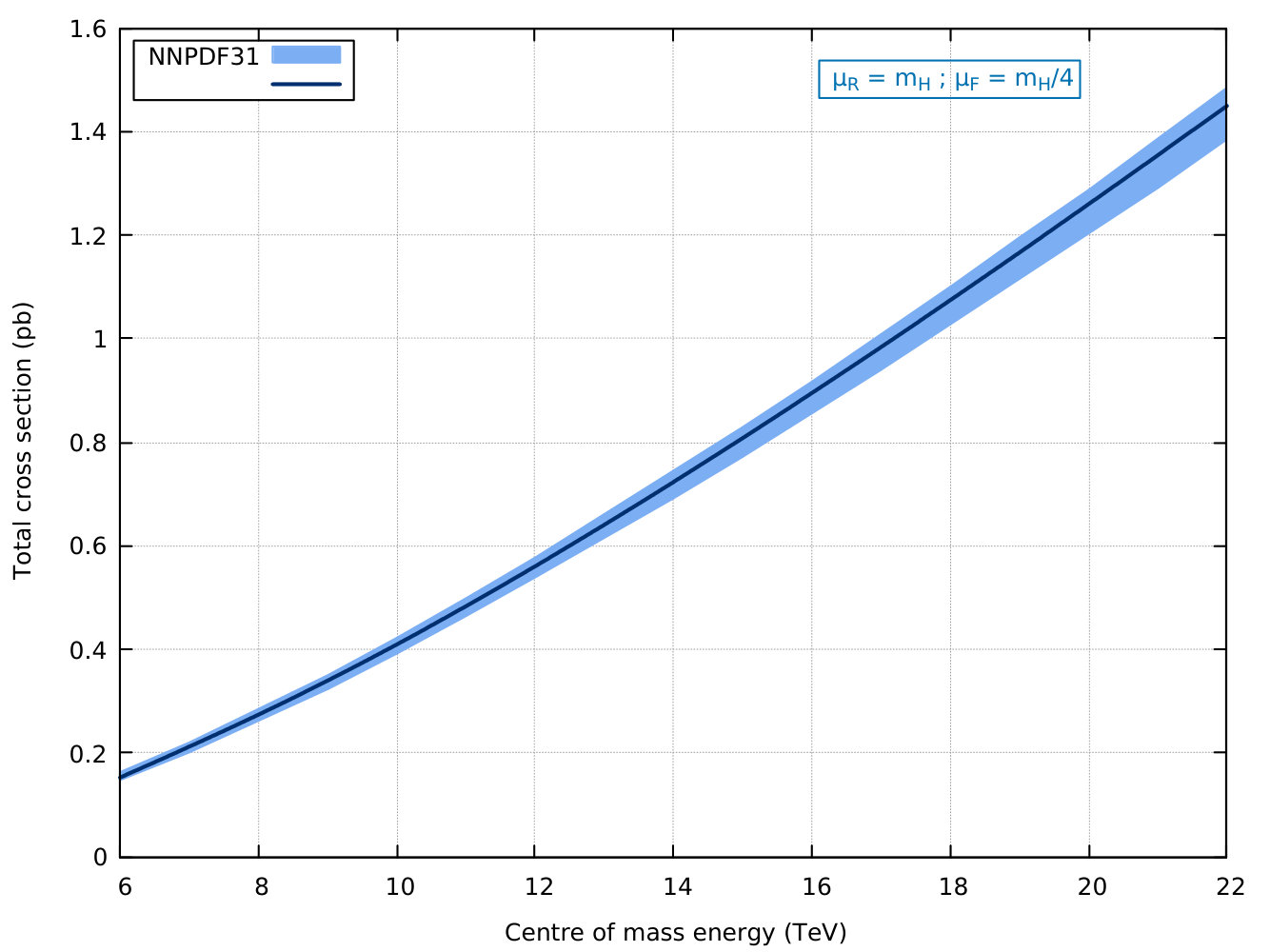 Figure 1
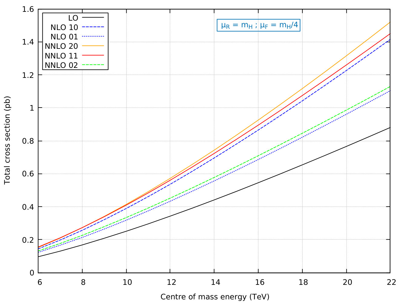 Figure 2
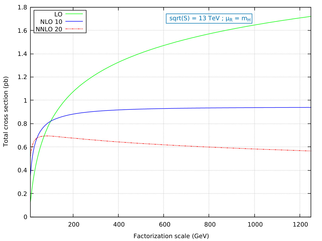 Figure 3
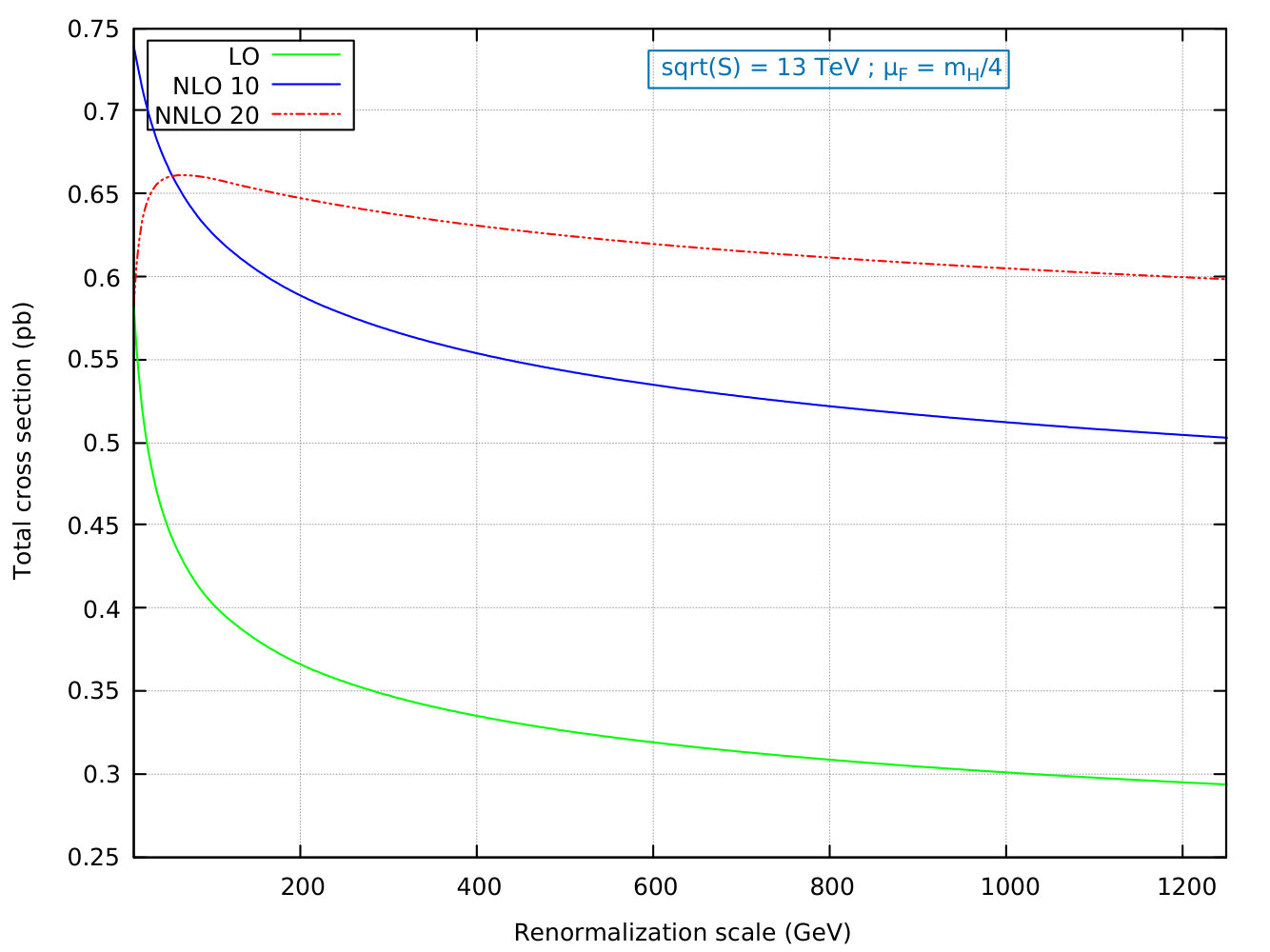 Figure 4
| LO00 | 1.0181 | |||||
|---|---|---|---|---|---|---|
| NLO10 | 1.1362 | -0.1810 | ||||
| NLO01 | 1.2219 | 0.0030 | ||||
| NNLO20 | 1.1433 | -0.1683 | -0.1935 | |||
| NNLO11 | 1.1542 | -0.1699 | 0.0029 | -0.0005 | ||
| NNLO02 | 1.2422 | 0.0031 | -4 |
| LO00 | 0.3911 | |||||
|---|---|---|---|---|---|---|
| NLO10 | 0.4588 | 0.1557 | ||||
| NLO01 | 0.4935 | 0.0003 | ||||
| NNLO20 | 0.4726 | 0.1614 | 0.0220 | |||
| NNLO11 | 0.4771 | 0.1630 | 0.0003 | 1.5 | ||
| NNLO02 | 0.5135 | 0.0003 | 6 |
| () | (2,) | (2,) | (1,) | (1,) | (1,) | (,) | (,) |
|---|---|---|---|---|---|---|---|
| NNLO20 (pb) | 0.707 | 0.643 | 0.690 | 0.656 | 0.562 | 0.661 | 0.606 |
| NNLO11 (pb) | 0.759 | 0.602 | 0.780 | 0.641 | 0.445 | 0.682 | 0.498 |
| NNLO02 (pb) | 0.728 | 0.465 | 0.804 | 0.514 | 0.250 | 0.574 | 0.279 |
| MRST | NNPDF | CT14 | PDF4LHC | |
|---|---|---|---|---|
| NNLO20 (pb) | 0.7805 | 0.7816 | 0.7574 | 0.8546 |
| NNLO11 (pb) | 0.9691 | 0.9867 | 0.9644 | 1.0625 |
| NNLO02 (pb) | 1.2020 | 1.2453 | 1.2288 | 1.3123 |
| MRST | NNPDF | CT14 | PDF4LHC | |
|---|---|---|---|---|
| NNLO20 (pb) | 0.6610 | 0.6561 | 0.6398 | 0.7178 |
| NNLO11 (pb) | 0.6451 | 0.6406 | 0.6259 | 0.6996 |
| NNLO02 (pb) | 0.5252 | 0.5139 | 0.5030 | 0.5605 |
Peer Reviews
No public reviews on file for this paper yet. If you reviewed it on a platform where reviews are public (OpenReview, ICLR, NeurIPS, ICML), you can paste yours below so the community can read it here.
Videos
No videos yet. Explain this paper in a talk, walkthrough, or lecture? Add one.
NNLO QCDQED corrections to Higgs production in bottom quark annihilation
Ajjath A H111E-mail: [email protected]
The Institute of Mathematical Sciences, HBNI, Taramani, Chennai 600113, India
Pulak Banerjee222E-mail: [email protected]
Paul Scherrer Institut, CH-5232 Villigen PSI, Switzerland
Amlan Chakraborty333E-mail: [email protected]
The Institute of Mathematical Sciences, HBNI, Taramani, Chennai 600113, India
Prasanna K. Dhani444E-mail: [email protected]
INFN, Sezione di Firenze, I-50019 Sesto Fiorentino, Florence, Italy
Pooja Mukherjee555E-mail: [email protected]
The Institute of Mathematical Sciences, HBNI, Taramani, Chennai 600113, India
Narayan Rana666E-mail: [email protected]
INFN, Sezione di Milano, Via Celoria 16, I-20133 Milan, Italy
V. Ravindran777E-mail: [email protected]
The Institute of Mathematical Sciences, HBNI, Taramani, Chennai 600113, India
Abstract
We present next-to-next-to leading order (NNLO) quantum electrodynamics (QED) corrections to the production of the Higgs boson in bottom quark annihilation at the Large Hadron Collider (LHC) in the five flavor scheme. We have systematically included the NNLO corrections resulting from the interference of quantum chromodynamics (QCD) and QED interactions. We have investigated the infrared (IR) structure of the bottom quark form factor up to two loop level in QED and in QCDQED using K+G equation. We find that the IR poles in the form factor are controlled by the universal cusp, collinear and soft anomalous dimensions. In addition, we derive the QED as well as QCDQED contributions to soft distribution function as well as to the ultraviolet renormalization constant of the bottom Yukawa coupling up to second order in strong coupling and fine structure constant. Finally, we report our findings on the numerical impact of the NNLO results from QED and QCDQED at the LHC energies taking into account the dominant NNLO QCD corrections.
††preprint: IMSc/2019/05/05, PSI-PR-19-12, TIF-UNIMI-2019-7
I Introduction
The discovery of the Standard Model (SM) Higgs boson by ATLAS Aad:2012tfa and CMS Chatrchyan:2012xdj collaborations at the Large Hadron Collider (LHC) has not only put the SM in a strong footing but also opened up a plethora of physics programs that can probe physics beyond the SM (BSM). Since the Higgs boson couples dominantly to heavy fermions and massive vector bosons, the corresponding observables are expected to be sensitive to new physics. In order to make definitive claims in the context of BSMs, it is henceforth extremely important to understand the Higgs sector of the SM. This is possible thanks to dedicated efforts from the LHC collaborations to measure the properties of the SM Higgs boson to unprecedented accuracy. Both ATLAS and CMS collaborations have already measured very precisely the partial width of the Higgs bosons both in the SM as well as in several BSM scenarios. This is the beginning of an era of precision physics at the LHC. These studies will be incomplete without the precise theoretical predictions in the SM as well as BSM.
At hadron colliders, where underlying scattering events are dominated by strong interaction, quantum effects are unavoidable. Quantum Chromodynamics (QCD), the theory of strong interaction, plays an important role at the LHC. Often, one finds that the leading order predictions from perturbative QCD are unreliable due to unphysical scales such as renormalization and factorization scales and also due to missing higher order radiative corrections. Radiative corrections from QCD are also large. Inclusion of such corrections improves the reliability of the predictions not only by making them more precise, but also by reducing the dependency on the unphysical scales.
At the LHC, the dominant production channel for the Higgs boson is gluon fusion through top quark loops Graudenz:1992pv . Owing to the complexities involved with the two loop massive Feynman integrals, an effective theory where top quark is integrated out, was proposed to obtain the first result at next-to-leading order (NLO) Dawson:1990zj for the Higgs boson production. Later on, in Djouadi:1991tka ; Spira:1995rr , the NLO corrections, taking into account the mass of the top quark, were shown to be very close to the prediction from the effective theory approach Dawson:1990zj . Thanks to the continued efforts beyond the NLO Harlander:2002wh ; Anastasiou:2002yz ; Ravindran:2003um ; Ravindran:2004mb ; Moch:2005ky ; Ravindran:2005vv ; Ravindran:2006cg , the most precise prediction till date, namely next-to-next-to-next-to leading order (N3LO) prediction Anastasiou:2015ema ; Mistlberger:2018etf for the inclusive production of the Higgs boson in the gluon fusion process, is now available (See Ravindran:2006bu ; Ahmed:2014uya ; Dulat:2018bfe for rapidity distributions). In addition, at NNLO accuracy, the tiny effects due to finite top quark mass have already been computed in Harlander:2009mq ; Pak:2009dg . Electroweak (EW) corrections Aglietti:2004nj ; Actis:2008ug and mixed QCD-EW corrections Anastasiou:2008tj are shown to improve the predictions.
The predictions from the perturbative QCD for the dominant production channel have reached the level of precision which now requires inclusion of the contributions from the sub-dominant channels. For example, one includes production channels such as vector boson fusion, associated production with a vector boson, bottom quark annihilation etc. In addition, the precise predictions deFlorian:2016spz taking into account radiative corrections from QCD and EW, are known for many of these processes.
Among these sub-dominant processes, production of the Higgs boson in bottom quark annihilation has been a topic of interest both in the SM as well as BSM contexts. In the SM, Yukawa couplings of the Higgs boson to the quarks and leptons are free parameters and precise determination of the couplings is possible at the LHC. These couplings are highly sensitive to scales of new physics as the mass () of the Higgs boson is close to the EW scale. Hence, both ATLAS ATLAS-CONF-2019-005 and CMS Sirunyan:2018koj collaborations have made dedicated efforts to measure them precisely. Among them, bottom Yukawa is one of the most sought one and it is a challenging task for experimentalists. Associated production of the Higgs boson with vector bosons or with top quarks and its subsequent decay to bottom quarks have been studied to achieve this. In addition, some interesting proposals can be found in Englert:2015dlp .
In the SM, bottom Yukawa coupling is less significant with respect to top Yukawa coupling while in the Minimal Supersymmetric SM (MSSM) Gunion:1992hs the coupling is proportional to which can increase the cross section in some parametric region. The angle is related to the ratio, denoted by , of the vacuum expectation values of two Higgs doublets. The production of Higgs boson(s) in perturbative QCD is studied in four flavor and five flavor schemes Buza:1996wv ; Bierenbaum:2009mv ; Blumlein:2018jfm , called 4FS and 5FS, respectively. In the former, one assumes that proton sea does not contain bottom quark, and they are radiatively generated from gluons in the proton. These bottom quarks can annihilate to produce the Higgs boson. Their contributions are enhanced by logarithms of bottom quark mass spoiling the perturbation theory. Hence they need to be resummed to obtain reliable predictions. In the 5FS, one can avoid these logarithms by introducing non-zero bottom quark distributions in the proton. They are present due to pair production of bottom quarks from the gluons in the proton sea. Since, the leading order contribution in 5FS is two to one, while in 4FS, it is two to three, computations beyond the leading order are relatively easier in 5FS. In 4FS, only NLO QCD effects Dittmaier:2003ej ; Dawson:2003kb ; Wiesemann:2014ioa are known. On the other hand, in 5FS, NLO Dicus:1998hs ; Balazs:1998sb , NNLO Harlander:2003ai and the threshold effects at N3LO Ravindran:2006cg ; Ahmed:2014cha (see Ravindran:2006bu ; Ahmed:2014era for rapidity distributions) are known for sometime. Also, 5FS cross-section providing the dominant cross-section in a matched prediction Bonvini:2016fgf ; Forte:2015hba is very well known. In Ebert:2017uel , resummation of time-like logarithms in SCET framework has been performed. Recently, for the bottom quark annihilation, complete N3LO corrections Gehrmann:2014vha ; Ahmed:2014pka ; Duhr:2019kwi have become available. In addition, the resummation of threshold contributions H:2019dcl at N3LO+N3LL accuracy have also been included.
Unlike the dominant channel, gluon fusion to the Higgs boson, bottom quark annihilation has not received much attention in the context of EW corrections, presumably because it is already sub-dominant at the LHC. In this paper, we make the first attempt to include the QED corrections to the inclusive production to this channel. We expect that these corrections could be comparable to the fixed Duhr:2019kwi and resummed H:2019dcl results solely from third order in perturbative QCD.
In deFlorian:2018wcj , pure QED and mixed QCDQED contributions have been obtained for the Drell-Yan (DY) process through Abelianization deFlorian:2015ujt ; deFlorian:2016gvk at orders and , respectively. In deFlorian:2018wcj , a suitable algorithm is obtained by studying the group theory structure of QCD and QED amplitudes that contribute to the partonic sub-processes of DY production. The algorithm contains a set of transformations on the color factors/Casimirs of SU(N) that transforms QCD results for the partonic sub-processes to the corresponding QED results. This way both pure QED as well as QCDQED contributions to inclusive production cross section for the Z boson in DY process have been obtained in deFlorian:2018wcj at NNLO level. Following this approach, we can in principle proceed to obtain pure QED and mixed QCDQED contributions to the bottom quark annihilation process from the QCD results. Although the QCD results Maltoni:2003pn ; Harlander:2003ai to NNLO are presented for of SU(N) and hence Abelianization can not be used, however, in Majhi:2010zg , resonant production of sleptons in a R-parity violating supersymmetric model was studied where radiative corrections from SU(N) gauge fields with fermions were included to NNLO level. Since, sleptons couple only to fermions in this model through Yukawa coupling, these NNLO corrections coincide with the results of Maltoni:2003pn ; Harlander:2003ai for . Hence, we could use the results given in Majhi:2010zg and method of Abelianization to obtain pure QED as well as QCD QED results for bottom quark annihilation to the Higgs boson. However, in order to scrutinize the very approach of Abelianization, we explicitly compute pure QED and QCDQED corrections to inclusive production of the Higgs boson in bottom quark annihilation up to NNLO level in U(1) and SU(N)U(1). In addition, we reproduce the same for the production of Z boson in DY process. The computation beyond the leading order involves evaluation of virtual and real emission processes. The contributions from them are sensitive to ultraviolet (UV) and infrared (IR) divergences. We compute them in dimensional regularization, hence divergences appear as poles in dimensional parameter , being the space-time dimension. The UV divergences are removed in scheme. The IR divergences result from soft gluons and massless collinear partons. The former is called the soft divergence and later collinear divergence. While soft divergences cancel between virtual and real emission processes in the inclusive cross section, the collinear divergences are removed by mass factorization. We determine, both UV as well as mass factorization counter terms using factorization property of the inclusive cross section and obtain collinear finite contributions to the Higgs boson production in bottom quark annihilation and Z boson production in DY. We determine IR anomalous dimensions up to two-loop level in both QED and QCDQED. We find that they are process independent. Using the universal IR anomalous dimension and following Ahmed:2015qpa , we compute the renormalization constant for the Yukawa coupling in QED as well as in QCDQED from the form factors (FF) of Higgs bottom anti-bottom operator and vector current of DY process.
The paper is organized as follows. In section II, after discussing the theoretical frame work, we briefly describe in sub-section II.1 how we compute higher order QCD and QED radiative corrections to various partonic and photonic channels that contribute to the inclusive cross section. In sub-section II.2, we discuss the UV and IR structure of the form factors and cross sections using K+G equation and obtain the mass factorized cross sections. In the following sub-section, we discuss about the Abelianization procedure. The phenomenological impact of our theoretical predictions are presented in section III. Finally we summarize in section IV. The universal constants that appear in soft distribution function, FFs of vector current and bottom quarks and the mass factorized partonic and photonic cross sections are presented in the Appendix A, B and C, respectively.
II Theoretical framework
The Lagrangian that describes the interaction of the Higgs boson with the bottom quarks is described by the Yukawa interaction and is given by
[TABLE]
where is the Yukawa coupling which, after the EW symmetry breaking, is found to be . and denote the bottom quark field and mass, respectively. is the vacuum expectation value (vev) of the Higgs field . In the SM, the Higgs boson production through bottom quark annihilation is sub-dominant compared to gluon fusion through top quark loop. One finds that the bottom Yukawa coupling is 35 times smaller than top quark Yukawa coupling and in addition, the bottom quark flux in the proton-proton collision is much smaller than the gluon flux. However, in the MSSM Nilles:1983ge , , the ratio of the vev s of Higgs doublets can increase the contributions resulting from the bottom quark annihilation channel. At LO,
[TABLE]
with
[TABLE]
where is the SM like light Higgs boson, and are the heavy and the pseudo-scalar Higgs bosons, respectively. The parameter is the mixing angle between weak and mass eigenstates of the neutral Higgs bosons and . We set except in the Yukawa coupling Aivazis:1993pi ; Collins:1998rz ; Kramer:2000hn as it is much smaller than the other energy scales in the process. The number of active flavors is taken to be and we work in the Feynman gauge.
The inclusive production of a colorless state in hadronic collisions is given by
[TABLE]
where is the Born cross section and are parton distribution functions (PDFs) for and photon distribution function (PHDF) if . The scaling variables is their momentum fractions. are the partonic sub-process contributions normalized by the Born cross section. The scales and are renormalization and factorization scales. and are hadronic and partonic center of mass energy, respectively. is the invariant mass of the final colorless state. can be expanded in powers of the QCD coupling constant and QED coupling constant , and being the strong and electromagnetic coupling constants, respectively. That is, after suppressing and dependence,
[TABLE]
with and . In the following, we describe the methodology to compute up to second order in the couplings.
II.1 Methodology
In this section, we briefly describe how higher order perturbative corrections (Eq. 5) are computed. The details of computational procedure can be found in Ahmed:2016qhu . Beyond the leading order (LO), the partonic channels consists of one and two loop virtual sub processes, real-virtual and single and double-real emissions, some of which are presented in Fig. 1, Fig. 2 and Fig. 3. The black line with an arrow indicates the bottom quark, the wavy line the photon, the curly line the gluon and the Higgs boson is indicated by the dashed line.
Sub-processes involving virtual diagrams are sensitive to UV singularities. Due to the presence of massless gluons and photons, we encounter soft singularities in both virtual and real emission sub-processes. In addition, we encounter collinear singularities, as we treat all the quarks including the bottom quark massless. We use dimensional regularization to regulate all these singularities.
\times$$\times
\times$$\times
\times$$\times$$\times
We have used the program QGRAF Nogueira:1991ex to generate virtual as well as real emission Feynman diagrams that contribute to the relevant sub-processes. An in-house FORM Vermaseren:2000nd code is used to perform all the symbolic manipulations, e.g. performing Dirac, SU(N) color and Lorentz algebra. Large number of loop integrals show up in the virtual diagrams. The integration-by-parts identities are used through a Mathematica based package, LiteRed Lee:2013mka to reduce them to a minimum set of master integrals. For those processes that involve pure real emissions with or without virtual diagrams, we use the method of reverse unitarity Anastasiou:2002yz that allows one to use IBP identities to reduce the resulting phase-space integrals to a set of few master integrals, the later can be found in Anastasiou:2012kq . Finally we obtain contributions to each sub-process, containing UV and IR singularities as poles in .
In the next section, we study the UV and IR structure of FF and the soft distribution function that contribute to NNLO level in QCD, QED and QCDQED. In order to explore the IR structure, we study the production of a boson in hadron colliders, namely DY process to the same accuracy in QCD, QED and QCDQED. In particular, we focus our attention to the FF and the soft distribution function that contribute to the inclusive DY production cross section. Following Ravindran:2006cg ; Ahmed:2015qpa ; Ahmed:2014cla , we demonstrate the factorization of IR singularities in both the FFs and show how to extract the process independent cusp (), collinear () and soft () anomalous dimensions from them. Using the FF of the bottom quark and the process independent soft distribution function we can extract the UV anomalous dimension of the Yukawa coupling up to two loop level in QCD, QED and QCDQED. Finally, we demonstrate the factorization of collinear singularities and the mass factorization leading to IR finite partonic contributions to inclusive hadronic cross sections for both the Higgs boson and DY productions up to NNLO level in QCD, QED and QCDQED.
II.2 UV and IR structures in QED and QCDQED
Having computed all the partonic channels that contribute to the hadronic cross sections in QED and QCDQED, we use them to study the UV and IR structure of the FFs and soft gluon/photon emissions in the Higgs boson and DY productions. For the former, we have used Sudakov K+G equation and for the later, following Ravindran:2005vv ; Ravindran:2006cg we exploited the universal structure of soft distribution function resulting from the soft gluon/photon emissions.
In order to remove the UV divergences that result from virtual sub-processes, we use the renormalization constants for the QCD and QED coupling constants, respectively and for the Yukawa coupling. The Yukawa coupling receives contributions from both QCD and QED. and relate the bare couplings of QCD and of QED to the renormalized ones and , respectively, at the renormalization scale in the following way,
[TABLE]
where . Here, is the phase-space factor in -dimensions, is the Euler-Mascheroni constant and is an arbitrary mass scale introduced to make and dimensionless in -dimensions. The renormalization constant up to two-loops are given by
[TABLE]
where and are QCD and QED beta functions, respectively. In the present case, only one loop i.e. and Cieri:2018sfk appear. They are given by
[TABLE]
Here, is the adjoint Casimir of . We also denote the fundamental Casimir for later use. is the number of active quark flavors and refers to electric charge for quark . The renormalization constant satisfies the renormalization group equation:
[TABLE]
whose solution in terms of the anomalous dimensions up to two loops is found to be
[TABLE]
Note that while the UV singularities factorize through , singularities from QCD and QED mix from two loop onward. For QCD, is known to four loops Vermaseren:1997fq . In this paper, using the universal IR structure of the amplitudes and cross sections in QED, we determine up to two loops in QED i.e. for and in QCDQED i.e. for .
We begin with the bare form factors , where denotes the DY process and denotes the Higgs boson production in bottom quark annihilation. Note that, these FFs are computed in the perturbative framework where both QCD as well as QED interactions are taken into account simultaneously and hence they depend on both QCD and QED coupling constants. In addition, we find that the UV renormalized FFs demonstrate the factorization of IR singularities. Using gauge and renormalization group invariance, we propose Sudakov integro-differential equation for these FFs, analogous to the QCD one. In dimensional regularization, they take the following form
[TABLE]
where and is the invariant mass of the final state particle (di-lepton pair in the case of DY and single Higgs boson for the case of Higgs production). Explicit computation of the form factors shows that IR singularities, resulting from QCD and QED interactions not only factorize but also mix beyond one loop level. In other words, if we factorize IR singularities from the FFs, the resulting IR singular function can not be written as a product of pure QCD and pure QED functions. More specifically, there will be terms proportional to , where , which will not allow factorization of QCD and QED ones. Hence, will have IR poles in from pure QED and pure QCD in every order in perturbation theory and in addition, from QCDQED starting from . On the other hand, overall factorization of IR singularities implies that the constants contain the IR singularities from QCD, QED and QCDQED, while the s will have IR finite contributions. Since, the IR singularities of FFs have dipole structure, will be independent of while s will be finite in and the later contain only logarithms in . Note that are renormalization group (RG) invariant so does the sum . Thus, the RG invariance of implies
[TABLE]
where are the cusp anomalous dimensions. The solutions to the above RG equations for can be obtained by expanding the cusp anomalous dimensions () in powers of renormalized coupling constants and as
[TABLE]
and as
[TABLE]
where and result from pure QCD and pure QED interactions and from QCDQED. Using RG equations for the couplings and , the perturbative solutions to Eq.(12) are found to be,
[TABLE]
Unlike , do not contain any IR singularities but depend only on and hence we expand them as
[TABLE]
where the first term is the boundary condition on each at . Expanding in powers of and and using RG equations for QCD and QED couplings, we obtain
[TABLE]
Expanding the finite function as,
[TABLE]
substituting the solutions of and in Eq.(II.2) and performing the integration over we get
[TABLE]
where,
[TABLE]
Following Ravindran:2004mb , we expand around in terms of collinear (), soft () and UV () anomalous dimensions as
[TABLE]
with
[TABLE]
The form factors that we computed in this paper in QCD, QED and QCDQED up to two loop level can be used to extract the cusp anomalous dimensions () by comparing them against Eq.(II.2). We find up to two loops as
[TABLE]
Unlike , the other anomalous dimensions , and ( is zero) can not be disentangled either from or alone. In order to disentangle and , we study the partonic cross sections resulting from soft gluon and soft photon emissions as they are only sensitive to .
To obtain the process independent part of soft gluon/photon contributions in the real emission sub-processes, we follow the method described in Ravindran:2005vv ; Ravindran:2006cg , where the soft distribution function for the inclusive cross section for producing a colorless state was obtained from the form factors and partonic sub-process cross sections involving real emissions of gluons. The soft distribution functions denoted by , are governed by cusp () and soft anomalous dimensions , where . It is also known that the identity holds up to three loop level Ravindran:2005vv ; Ravindran:2006cg ; Ahmed:2014cla . We can use the partonic sub-processes of either DY process or the Higgs boson production in bottom quark annihilation namely or normalized by the square of the bare form factor or to obtain . In general , which is function of the scaling variable , is defined as,
[TABLE]
with and being the overall renormalization constant. The symbol refers to “ordered exponential” which has the following expansion:
[TABLE]
Here is the Mellin convolution and is a distribution of the kind and . The plus distribution is defined as,
[TABLE]
We can compute the UV finite every order in renormalized perturbation theory. Since, we have not determined , we can only compute the unrenormalized partonic cross section . From the explicit results for and the form factors , using Eq. (25) we obtain up to second order in , and . We find up to second order in the couplings demonstrating the universality. In Ravindran:2005vv ; Ravindran:2006cg , it was shown that the soft distribution function satisfies Sukakov K+G equation analogous to the form factor due to similar IR structures that both of them have, order by order in perturbation theory. That is, satisfies
[TABLE]
where, the IR singularities are contained in and the finite part in . RG invariance of implies
[TABLE]
Note that, the same anomalous dimensions govern the evolution of both and . This ensures that the soft distribution function contains right soft singularities to cancel those from the form factor leaving bare partonic cross section to contain only initial state collinear singularities. The later will be removed by mass factorization by appropriate Altarelli-Parisi kernels. Expanding and in powers of as has been done for and (see Eqs.(15,19)), with the replacements of by and
[TABLE]
the solution to Eq.(II.2) is found to be
[TABLE]
where,
[TABLE]
is related to finite function defined in Eq.(30) through the distributions and . Thus expanding in terms of the and we write,
[TABLE]
where . Following, Ravindran:2005vv ; Ravindran:2006cg , the IR finite can be expanded as
[TABLE]
where, for up to two loops
[TABLE]
Comparing the soft distribution functions , , obtained from the explicit computation up to second order in coupling constants against the formal solution given in Eqs.(II.2), we can obtain and for . Finally, we obtain and
[TABLE]
Now that we have , it is now straightforward to obtain in Eq.(22) from the explicit results on as for DY. This way we obtain,
[TABLE]
Assuming , we determine the UV anomalous dimension, from (Eq.(22)) which is known to second order. They are found to be
[TABLE]
Alternatively, assuming and , we can determine by comparing the difference obtained using DY and Higgs boson form factors and at against the formal decomposition of given in Eqs.(22). Substituting the above UV anomalous dimensions in Eq.(II.2), we obtain to second order in the couplings.
Using the renormalization constants , and for the coupling constants , and the Yukawa coupling , we obtain UV finite partonic cross sections. The soft and collinear singularities arising from gluons/photons/fermions in the virtual sub-processes cancel against those from the real sub-processes when all the degenerate states are summed up, thanks to the KLN theorem Kinoshita:1962ur ; Lee:1964is . What remains at the end, is the initial state collinear singularity, which can be removed by mass factorization. Collinear factorization allows us to determine the mass factorization kernels and up to two-loop level for and cases. Since and are governed by the splitting functions and , we extract them to second order in couplings. In deFlorian:2015ujt , these splitting functions up to NNLO level, both in QED and QCDQED, were obtained using the Abelianization procedure. The splitting functions that we have obtained by demanding finite-ness of the mass factorised cross section, agree with those in deFlorian:2015ujt . The mass factorized partonic cross section for each partonic sub-process up to NNLO in QED and in QCDQED are presented in the Appendix along with the known NNLO QCD results Harlander:2003ai . In the next section, we use them to study their numerical impact at the LHC energies.
II.3 Abelianization procedure
In deFlorian:2018wcj , QCDQED corrections to the DY process were obtained by studying the color factors in Feynman diagrams that contribute to QCD corrections. This led to an algorithm namely Abelianization procedure which provides a set of rules that transform QCD results into pure QED and mixed QCDQED results. Unlike in deFlorian:2018wcj , without resorting to Abelianization rules, we have performed explicit calculation to obtain the contributions resulting from all the partonic and photonic channels taking into account both UV and mass factorization counter terms. Using these results at NNLO in QCD, QCDQED and in QED, we find a set of rules that can relate QCD and QED results. Note that if there is a gluon in the initial state, averaging over its color factor gives a factor . This is absent for the processes where photon is present instead of gluon in the initial state. Also, for pure QCD or QED, the gluons or photons are degenerate and hence one needs to account for a factor of 2. Keeping these in mind, we arrive at a set of relations among QCD and QED results. We have listed them in the following tables for various scattering channels. They are found to be consistent with the procedure used in deFlorian:2018wcj .
Rule 1 : quark-quark initiated cases
[TABLE]
when both initial quarks are bottom quarks.
Rule 2 : *quark-gluon initiated cases
*(After multiplying for the initial state gluon)
[TABLE]
Rule 3 : *gluon-gluon initiated cases
*(After multiplying for each initial state gluon)
[TABLE]
III Results and phenomenology
In this section, we study the numerical impact of pure QED and mixed QCDQED corrections over the dominant QCD corrections up to NNLO level to the production of the Higgs boson in bottom quark annihilation at the LHC, mainly for the center of mass (CM) energy of TeV. Since we include QED effects, we need PHDF inside the proton in addition to the standard PDFs. For this purpose, we use NNPDF 3.1 LUXqed set Bertone:2017bme , MRST Martin:2004dh , CT14 Schmidt:2015zda and PDF4LHC17. The PDFs, PHDFs and the strong coupling constant can be obtained, using the LHAPDF-6 Buckley:2014ana interface. We have used the following input parameters for the masses and the couplings:
[TABLE]
Both and are evolved using appropriate QCD -function coefficients and quark mass anomalous dimensions respectively. However, we have considered fixed throughout the computation.
The Higgs boson production cross section from bottom quark annihilation at the present energy of LHC is not substantial. However, for the high luminosity LHC, measuring them at higher center of mass energy (CM) would give larger contributions and it will improve the precision. Hence, we have first studied how the cross section varies with the CM of LHC. In Fig. 4, we plot the inclusive production cross sections at various orders in perturbative QCD and QED for the range of CM energies between to TeV. In the inset, the index ‘ij’ indicates that QCD at ‘i’- order and QED at ‘j’- order in perturbative theory are included (e.g. ‘NNLO 11’ indicates NNLO mixed QCDQED). In Fig. 4, we have used NNPDF31_lo_as_0118, NNPDF31_nlo_as_0118_luxqed and NNPDF31_nnlo_as_0118_luxqed for LO, NLO and NNLO, respectively. The renormalization () and factorization () scales are kept fixed at and , respectively. We note that in Fig. 4, the pure QED contributions are large. This is due to the fact that we consider leading order QCD running of Yukawa coupling which gives larger Born contribution compared to pure QCD. In order to understand this in more detail, we study the impact of different contributions to the cross sections resulting from QCD, QED and mixed QCDQED at various orders in perturbation theory which we have tabulated in Table 1, for TeV and for the scale choice .
The indicates sole -th order QCD and -th order QED corrections to the total contribution. For example, NNLO11 means .
In Table 2, a similar study has been performed for TeV and the scales .
Fixed order predictions depend on the renormalization () and factorization () scales. The uncertainty resulting from the choice of the scales quantify the missing higher order contributions. Hence, we have studied their dependence by varying them independently around a central scale.
Fig. 5 shows the dependence of the cross section on the renormalization scale () for the fixed choice of the factorization scale . It clearly demonstrates the importance of higher order corrections as the variation is much more stable at NNLO20 compared to the lower orders.
In Fig. 6, we present the dependence on the factorization scale () keeping the renormalization scale () fixed at . Similar to the variation, variation improves after adding higher order corrections. To illustrate their dependence when both the scales are changed simultaneously, we present the cross section by performing 7-point scale variation and the results are listed in Table 3. We have used NNPDF31_nnlo_as_0118_luxqed for this study.
The perturbative predictions also depend on the choice of PDFs and PHDFs. There are several groups which fit them and are widely used in the literature for the phenomenological studies. In order to estimate the uncertainty resulting from the choice of PDFs and PHDFs, in Table 4, we present the NNLO results from various PDF sets, for =14 TeV and .
In Table 5, we repeat the study for =13 TeV and and .
We have also studied the uncertainties resulting from the choice of PDF set Buckley:2014ana . Using NNPDF31, in Fig 7, we plot the variation of the cross section with respect to different choices of PDF and PHDF templates keeping the central set as the reference. The thick line is obtained using the central set. The shaded region resulting from other sets quantifies the uncertainty.
IV Discussion and Conclusion
Precision studies is one of the prime areas at the LHC. Measuring the parameters of the SM to unprecedented accuracy can help us to improve our understanding of the dynamics that governs the particle interactions at high energies. This is possible only if the accuracy of theoretical predictions is comparable to that of the measurements. Thanks to the on-going efforts from experimentalists and theorists, there are stringent constraints on various physics scenarios in the pursuit of searching for the physics beyond the SM. The efforts to compute the observables that are related to top quarks and Higgs bosons have been going on for a while as these observables are sensitive to high scale physics. Since the dominant contributions to these processes are known to unprecedented accuracy, inclusion of sub-dominant contributions along with radiative corrections is essential for any consistent study. In this context, the present article explores the possibility of including EW corrections to Higgs boson production in bottom quark annihilation which is sub-dominant. Note that, this is known to third order in QCD Duhr:2019kwi . While this is a sub-dominant process at the LHC, in certain BSM contexts, the rates are significantly appreciable leading to interesting phenomenological studies. Since, the computation of full EW corrections is more involved, as a first step towards this, we compute all the QED corrections, in particular, to the inclusive Higgs boson production in bottom quark annihilation up to second order in QED coupling constant , taking into account the non-factorizable or mixed QCDQED effects through corrections. The computation involves dealing with QED soft and collinear singularities resulting from photons and the massless partons along with the corresponding QCD ones. Understanding the structure of these QED IR singularities in the presence of QCD ones, is a challenging task. We have systematically investigated both QCD and QED IR singularities up to second order in their couplings taking into account the interference effects. We use Sudakov K+G equation to understand the IR structure in terms of cusp, colliner and soft anomalous dimensions. We demonstrate that the IR singularities from QCD, QED and QCDQED interactions factorize both at the FF, as well as at the cross section level. While the IR singularities factorize as a whole, the IR singularities from QCD do not factorize from that of QED leading to mixed/non-factorizable QCDQED IR singularities. In addition, by computing the real emission processes in the limit when the photons/gluons become soft, we have studied the structure of soft distribution function. While the later demonstrates the universal structure analogous to QCD one, we find that it contains soft terms from mixed QCDQED that do not factorize either as a product of those from QCD and QED separately. Using the universal IR structure of the observable, we have determined the mass anomalous dimension of the bottom quark and hence the renormalization constant for the bottom Yukawa. We also discussed the relation between the results from pure QED and pure QCD as well as between QCDQED and QCD through Abelianization. We have determined a set of rules that relate them and they are found to be consistent with those observed in the context of DY deFlorian:2018wcj . Having obtained the complete NNLO results from QED and QCDQED, we have systematically included them in the NNLO QCD study to understand their impact at the LHC energy. We find that the corrections are mild as expected. However, we show that the higher order corrections from QED and QCDQED improve the reliability of the predictions.
Acknowledgment
A.A.H, A.C, P.M and V.R would like to acknowledge the support of the CNRS LIA (Laboratoire International Associé) THEP (Theoretical High Energy Physics) and the INFRE-HEPNET (IndoFrench Network on High Energy Physics) of CEFIPRA/IFCPAR (Indo-French Centre for the Promotion of Advanced Research). We thank G. Ferrera and A. Vicini for useful discussions.
Appendix A s of the soft distribution function
The constants in the soft distribution function are given by,
[TABLE]
Appendix B Form factors
We present the analytic expressions of the form factors and the finite partonic cross sections for all the partonic channels. The labeling is same as Fig. 4
The unrenormalized form factor () can be written as follows in the perturbative expansion of unrenormalized strong coupling constant () and unrenormalized fine structure constant ()
[TABLE]
denotes the Drell-Yan pair production and the Higgs boson production in bottom quark annihilation, respectively. The coefficients and are
[TABLE]
The coefficients and are
[TABLE]
Appendix C for bottom quark annihilation from QCD, QED and QCDQED up to NNLO
In the following, we present finite partonic cross sections as defined in Eq. 5, up to NNLO level in the strong and electro-magnetic coupling constants. In QCD, for bottom quark annihilation is already known Harlander:2003ai ; Majhi:2010zg . In the following, is in gauge theory, while is in gauge theory.
[TABLE]
The corresponding results from the QED and QCDQED are found to be
[TABLE]
Partonic cross sections contributing to pure NLO and NNLO QED corrections:
[TABLE]
The constants , denote the Riemann’s -functions, e.g., and . The Spence functions Li and Li are defined by
[TABLE]
and the Nielson function S is given by
[TABLE]
The reference list from the paper itself. Each links out to its DOI / PubMed record.
- 1(1) ATLAS collaboration, G. Aad et al., Observation of a new particle in the search for the Standard Model Higgs boson with the ATLAS detector at the LHC , Phys. Lett. B 716 (2012) 1–29 , [ 1207.7214 ]. · doi ↗
- 2(2) CMS collaboration, S. Chatrchyan et al., Observation of a new boson at a mass of 125 Ge V with the CMS experiment at the LHC , Phys. Lett. B 716 (2012) 30–61 , [ 1207.7235 ]. · doi ↗
- 3(3) D. Graudenz, M. Spira and P. M. Zerwas, QCD corrections to Higgs boson production at proton proton colliders , Phys. Rev. Lett. 70 (1993) 1372–1375 . · doi ↗
- 4(4) S. Dawson, Radiative corrections to Higgs boson production , Nucl. Phys. B 359 (1991) 283–300 . · doi ↗
- 5(5) A. Djouadi, M. Spira and P. M. Zerwas, Production of Higgs bosons in proton colliders: QCD corrections , Phys. Lett. B 264 (1991) 440–446 . · doi ↗
- 6(6) M. Spira, A. Djouadi, D. Graudenz and P. M. Zerwas, Higgs boson production at the LHC , Nucl. Phys. B 453 (1995) 17–82 , [ hep-ph/9504378 ]. · doi ↗
- 7(7) R. V. Harlander and W. B. Kilgore, Next-to-next-to-leading order Higgs production at hadron colliders , Phys. Rev. Lett. 88 (2002) 201801 , [ hep-ph/0201206 ]. · doi ↗
- 8(8) C. Anastasiou and K. Melnikov, Higgs boson production at hadron colliders in NNLO QCD , Nucl. Phys. B 646 (2002) 220–256 , [ hep-ph/0207004 ]. · doi ↗